Observational appearances of isolated stellar-mass black hole accretion - theory and observations

Abstract

General properties of accretion onto isolated stellar mass black holes in the Galaxy are discussed. An analysis of plasma internal energy growth during the infall is performed. Adiabatic heating of collisionless accretion flow due to magnetic adiabatic invariant conservation is $25\%$ more efficient than in the standard non-magnetized gas case. It is shown that magnetic field line reconnections in discrete current sheets lead to significant nonthermal electron component formation, which leads to a formation of a hard (UV, X-ray, up to gamma), highly variable spectral component in addition to the standard synchrotron optical component first derived by Shvartsman generated by thermal electrons in the magnetic field of the accretion flow. Properties of accretion flow emission variability are discussed. Observation results of two single black hole candidates - gravitational lens MACHO-1999-BLG-22 and radio-loud x-ray source with featureless optical spectrum J1942+10 - in optical band with high temporal resolution are presented and interpreted in the framework of the proposed model.

1 Accretion onto isolated stellar-mass black holes

Even though more than 60 years have passed since the theoretical prediction of black holes as an astrophysical objects (Oppenheimer&Snyder, 1939) in some sense they have not been discovered yet.

The features of the black hole – the compactness (the size for the mass $M$ is close to the Schwarzschild one $r_{g}=\frac{2GM}{c^{2}}$ and the mass larger than 3$M_{\odot}$ – are the necessary, but not the sufficient ones. The deciding property of the black hole is the presence of the event horizon, instead of with the usual surface. To decide whether it is present in a given compact and massive object it is necessary to detect and study the emission generated very near the event horizon.

It is a very complicated task that cannot be easily performed in x-ray binaries and AGNs due to high accretion rate and so the high optical depth of the accreting gas. At the same time, single stellar-mass black holes, which accrete interstellar medium of low density ($10^{-2}-1$cm^-3), are the ideal case for detection and study of the event horizon (Shvartsman, 1971).

The analysis of existing data on possible black hole masses and velocities in comparison with the interstellar medium structure shows that in the majority of cases in the Galaxy ($>90\%$) the accretion rate $\dot{m}=\dot{M}c^{2}/L_{edd}$ can’t exceed $10^{-6}-10^{-7}$ (Beskin & Karpov, 2005).

Black holes usually move supersonically (at Mach numbers 2-3). And only in cold clouds of the interstellar hydrogen ($n\sim 10^{2}-10^{5}$, $T\sim 10^{2}$) and at low velocities of motion ($<10$ km/s) the accretion rates may be high and black hole luminosities may reach $10^{38}-10^{40}$ erg/c. For typical interstellar medium inhomogeneity the captured specific angular momentum is smaller than that on the BH last stable orbit, and the accretion is always (with the exception of the case of a black hole in a dense molecular cloud) spherically-symmetric (Mii&Totani, 2005; Beskin & Karpov, 2006).

The accreting plasma is initially collisionless, and it remains so until the event horizon. The electron-electron and electron-ion free path $\lambda\sim 2.4\cdot 10^{3}T^{2}n^{-1}$ even at the capture radius is as high as $\sim 10^{12}$ cm. Only the magnetic fields trapped in plasma (the proton Larmor radius at $r_{g}$ is 10 cm) make it possible to consider the problem as a quasi-hydrodynamical one; it is only due to the magnetic field that the particle’s momentum is not conserved, allowing particles to fall towards the black hole. In addition, the magnetic field effectively ”traps” particles in a ”box” of variable size, which allows us to consider its adiabatic heating during the fall; a correct treatment of such a process shows that for magnetized plasma such heating is 25% more effective than for ideal gas due to the conservation of magnetic adiabatic invariant $I=\frac{3cp_{t}^{2}}{2eB}$, where $p_{t}$ is the tangential component of electron momentum(Beskin & Karpov, 2005). Therefore, the plasma temperature in the accretion flow grows much faster and electrons become relativistic earlier – $R_{rel}\approx 6000$ in contrast to $R_{rel}\approx 1300$ in Bisnovatyi-Kogan & Ruzmaikin (1974) and $R_{rel}\approx 200$ in Ipser & Price (1982). The accretion flow is much hotter, and our estimation of ”thermal” luminosity

$$L=\eta\dot{M}c^{2}=9.6\cdot 10^{33}M_{10}^{3}n_{1}^{2}(V^{2}+c_{s}^{2})_{16}^{-3}\mbox{ erg/s}$$ (1)

is significantly higher than those of Ipser & Price (1982)

$$L_{\rm IP}=1.6\cdot 10^{32}M_{10}^{3}n_{1}^{2}(V^{2}+c_{s}^{2})_{16}^{-3}\mbox{ erg/s}$$ (2)

and Bisnovatyi-Kogan & Ruzmaikin (1974)

$$L_{\rm BKR}=2\cdot 10^{33}M_{10}^{3}n_{1}^{2}(V^{2}+c_{s}^{2})_{16}^{-3}\mbox{ erg/s, }$$ (3)

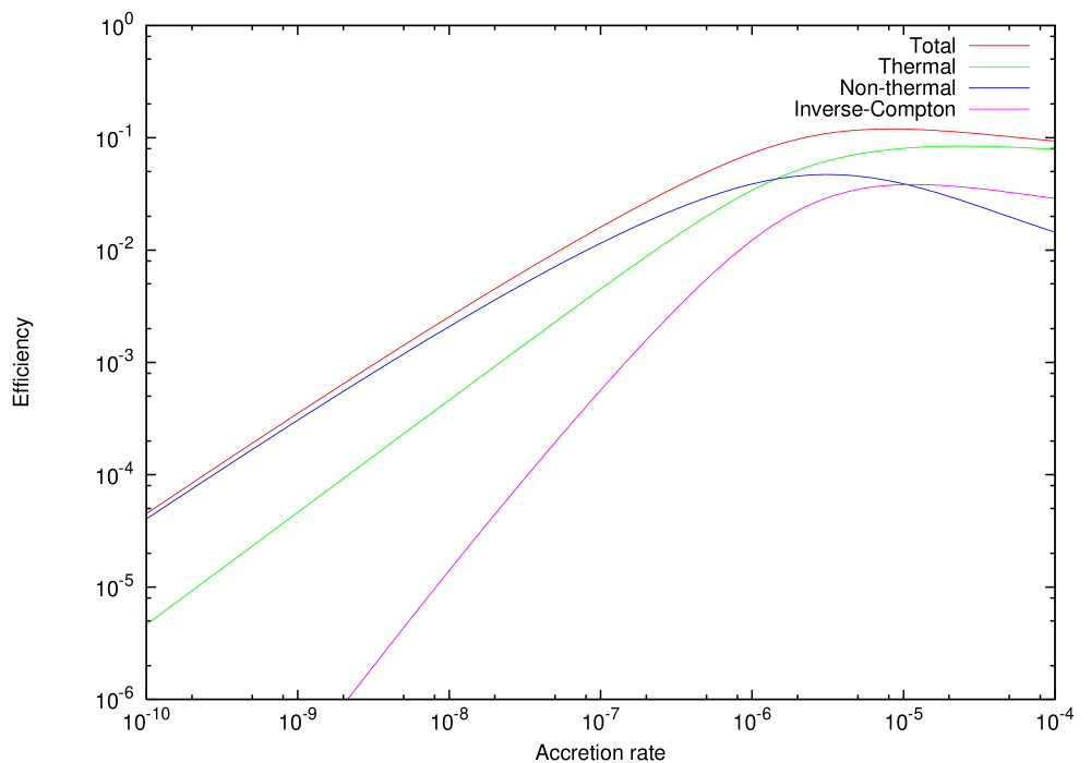
Figure 5: Efficiencies of the synchrotron emission of thermal and non-thermal electron components of the accretion flow.

while the optical spectral shape is nearly the same. The efficiency of accretion as a function of accretion rate is shown in Fig. 5.

The basis of our analysis is the assumption of the energy equipartition in the accretion flow (Shvartsman’ theorem, see Shvartsman (1971)). The straight consequence of this assumption is the necessity of exceeding magnetic energy dissipation with the rate

$$\frac{dE}{dVdt}=4\frac{v}{r}\frac{B^{2}}{8\pi}-\frac{5}{2}\frac{v}{r}\frac{B^{2}}{8\pi}=\frac{3}{2}\frac{v}{r}\frac{B^{2}}{8\pi}.$$ (4)

In the previous accretion models the dissipation goes continuously(Bisnovatyi-Kogan & Lovelace, 1997) in the turbulent flow and its mechanism is not examined in details. We considered conversion of the magnetic energy in the discrete turbulent current sheets (Pustilnik, 1997) as a mechanism providing such dissipation. At the same time, various modes of plasma oscillations are generated (ion-acoustic and Lengmur plasmons mostly), magnetic field lines reconnect and are ejected with plasma from the current sheet and electrons are accelerated. The latter effect is very important for the observational appearances of the whole accretion flow. The beams of the accelerated electrons emit its energy due to motion in the magnetic field and generate an additional (in respect to synchrotron emission of thermal particles) nonthermal component.

Current sheet spatial scales are usually much smaller than the whole accretion flow one and, therefore, the fraction of the accelerated particles is small, and so the total (significantly nonthermal) electron distribution $f(R,\gamma)$ may be considered as a superposition of the purely thermal one $f_{t}(R,\gamma)$ for the background flow particles and purely nonthermal $f_{nt}(R,\gamma)$ for the ones accelerated in the current sheets (this is the approach known as ”hybrid plasma”, see Coppi (1999)). Also we assume that for low accretion rates the non-adiabatic heating and radiative energy losses do not change the shape of the thermal component distribution (while changing its mean energy), then

$$f(R,\gamma)=f_{t}(R,\gamma)+\zeta f_{nt}(R,\gamma).$$ (5)

Note that this distribution is not normalized, and only its shape has physical meaning. So, for example, the ratio of nonthermal to thermal electron densities at some radius $R$ may be expressed as

$$\frac{n_{nt}(R)}{n_{t}(R)}=\frac{\zeta f_{nt}(R)}{f_{t}(R)}\mbox{ ,}$$ (6)

where $f_{nt}(R)$ and $f_{t}(R)$ are integrals of the corresponding distribution functions over the range of $\gamma$.

Thermal particle distribution function may be written as

$$f_{t}(R,\gamma)=\frac{\sqrt{R}}{2\tau}\left(\frac{\gamma}{\tau}\right)^{2}\exp{\left(-\frac{\gamma}{\tau}\right)},$$ (7)

where the usual dimensionless expression for temperature $\tau=kT/m_{e}c^{2}$ is used. This gives a Maxwellian local energy distribution and radial density slope ${\rho\propto R^{-3/2}}$.

To get the temperature profile of the accretion flow let’s take into account that the fraction $\xi\sim 0.1$ of the magnetic field energy during its dissipation is converted to the energy of the accelerated particles. Then, according to (4), the non-adiabatic heating rate may be expressed as

$$\Phi=(1-\xi)\frac{dE}{dVdt}=(1-\xi)\frac{3}{2}\frac{v}{r}\frac{B^{2}}{8\pi}\mbox{ .}$$ (8)

The main mechanism of radiative losses at low accretion rates is synchrotron radiation. Its rate may be written as (Lightman&Rybicki, 1979)

$$\Lambda_{sync}=\frac{4}{3}\sigma_{T}c\overline{\gamma^{2}}\frac{B^{2}}{8\pi}n.$$ (9)

For a Maxwellian distribution

$$\overline{\gamma^{2}}=12\left(\frac{kT}{m_{e}c^{2}}\right)^{2}=12\tau^{2}.$$ (10)

For relatively large accretion rates ($\dot{m}>10^{-6}$) it is necessary to take into account the cooling due to inverse Compton effect, which converts the part of hot electrons energy to the hard emission.

The rate of inverse Compton energy losses is related to the synchrotron one as (Lightman&Rybicki, 1979)

$$\Lambda_{compton}=\Lambda_{sync}\frac{\epsilon_{rad}}{B^{2}/8\pi}$$ (11)

Taking into account non-adiabatic terms, the energy balance equation per particle may be written for a non-relativistic region of the flow ($R>R_{rel}$) as

$$\frac{d}{dr}\frac{\epsilon}{n}=-\frac{5}{4}\frac{\epsilon}{nr}+\frac{1}{v}\frac{\Lambda-\Phi}{n}\mbox{ .}$$ (12)

For a non-relativistic electron gas $\epsilon=\frac{3}{2}nkT$, so

$$\frac{d\tau}{dR}=-\frac{5}{4}\frac{\tau}{R}-(1-\xi)\frac{\alpha^{2}}{2}\frac{m_{p}}{m_{e}}R^{-2},$$ (13)

while for the relativistic one ($\epsilon=3p=3nkT$)

$$\frac{d\tau}{dR}=-\frac{5}{8}\frac{\tau}{R}-(1-\xi)\frac{\alpha^{2}}{4}\frac{m_{p}}{m_{e}}R^{-2}+\frac{4}{3}\frac{m_{p}}{m_{e}}\frac{\dot{m}\tau^{2}}{R^{2}},$$ (14)

where $\alpha^{2}=\frac{1}{3}$ (the equipartition condition).

The boundary condition is ${\tau(R_{rel})=1}$.

An analytical solution of this equation in general is very difficult, but for low accretion rates we may neglect the influence of radiative losses and get a solution in the form

$$\tau(R)=(1-\xi)\frac{2\alpha^{2}}{3}\frac{m_{p}}{m_{e}}R^{-1}+\left(1-(1-\xi)\frac{2\alpha^{2}}{3R_{rel}}\frac{m_{p}}{m_{e}}\right)\left(\frac{R_{rel}}{R}\right)^{5/8}.$$ (15)

This expression may be substituted into (7) to get the final expression for the thermal electron distribution.

The energy evolution of single nonthermal electron is described by

$$\frac{d\gamma}{dR}=\frac{1}{3}\frac{m_{p}}{m_{e}}\dot{m}\frac{\gamma^{2}}{R^{2}}-\frac{5}{8}\frac{\gamma}{R},$$ (16)

where the first term corresponds to synchrotron losses and the second one to adiabatic heating.

Analysis of the evolution of electron beams ejected from the current sheets (Beskin & Karpov, 2005) gives the possibility to compute the $\xi$ and $f_{nt}(R,\gamma)$, i.e. the fraction of thermal and nonthermal component contributions to the total one.

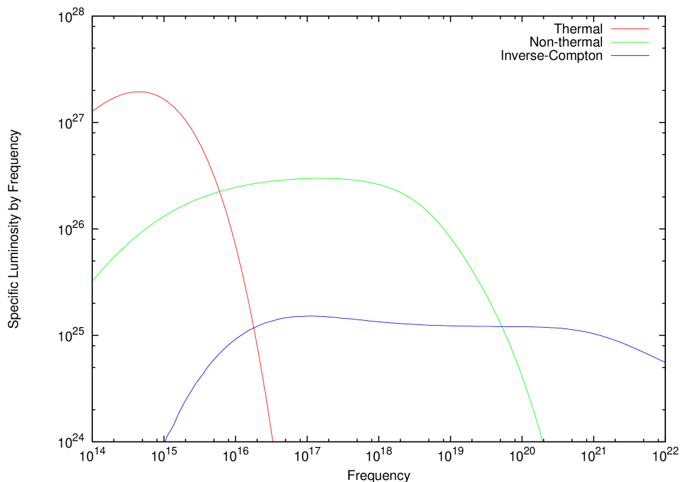
Figure 1: Decomposition of a single black hole (with the mass $10M_{\odot}$) emission spectrum into thermal and nonthermal parts. The accretion rate is $1.4\cdot 10^{10}$ g/s, which corresponds to $\dot{m}=10^{-8}$.

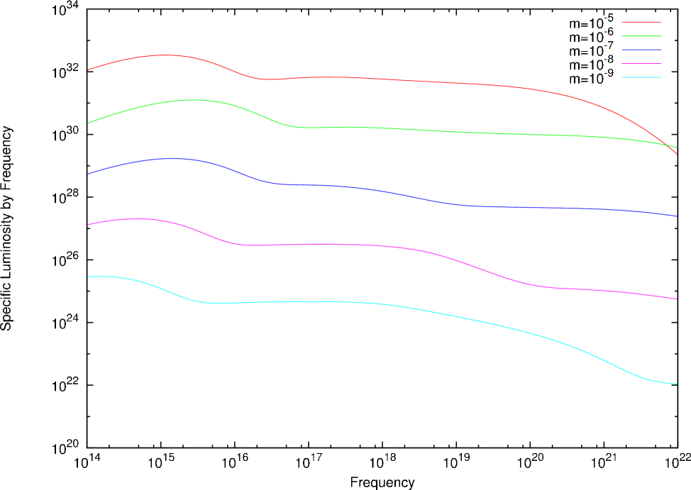
Figure 2: Spectra of the accretion flow onto the 10 $M_{\odot}$ black hole for the various accretion rates.

The spectra of various components of the accretion flow emission have been computed taking into account relativistic effects of emission propagation near the black hole (Lightman&Rybicki, 1979; Shapiro, 1973). They are shown in Fig. 2 for various accretion rates. In Fig. 3 the integral dependence of the thermal emission of accretion flow on the distance to the black hole is presented. The large fraction of it is generated inside the 2$r_{g}$ sphere, and so carries the information very near the event horizon.

Figure 3: Fraction of thermal synchrotron emission that comes from inside a given radius $R$

An important property of the nonthermal emission is its flaring nature – the electron ejection process is discrete, and typical light curve of single beam is shown in Fig. 4. The light curve of each such flare has a stage of fast intensity increase and sharp cut-off, its shape reflects the properties of the magnetic field and space-time near the horizon.

The black hole at a 100 pc distance (a sphere with this radius must contain several tens of such objects, see (Agol & Kamionkowski, 2002)) looks like a 15-25^m optical object (due to the ”thermal” spectral component) with a strongly variable companion in high-energy spectral bands (”nonthermal” component). The hard emission consists of flares, the majority of which are generated inside a 5$r_{g}$ distance from the BH. These events have the durations $\sim r_{g}/c$ ($\sim$ 10^-4 s), a rate of 10³-10⁴ flares per second, and an amplitude of 2%-6%. The BH variable X-ray emission may be detected by modern space-borne telescopes.

Optical emission consists of both a quasistationary ”thermal” part and a low-frequency tail of nonthermal flaring emission. The rate and duration of optical flares are the same as X-ray ones, while their amplitudes are significantly smaller. Indeed, the contribution of nonthermal component to the optical emission is approximately $2\cdot 10^{-2}$ for $\dot{m}=10^{-8}-10^{-6}$, so the mean amplitudes of optical flares are 0.04%-0.12%, while the peak ones may be 1.5-2 times higher and reach 0.2%. Certainly, it is nearly impossible to detect such single flares, but their collective power reaches 18-24^m and thus may be detected in observations with high time resolution ($<$ 10^-4 s) by the large optical telescopes(Beskin & Karpov, 2005).

Of course, the variability of the BH emission is related not only to the electron acceleration processes described here. Additional variability may be result of the plasma oscillations of different kinds, or other types of instabilities. The time scale of such variability may be from $r_{g}/c$ till $r_{c}/c$, i.e. from microseconds till years.

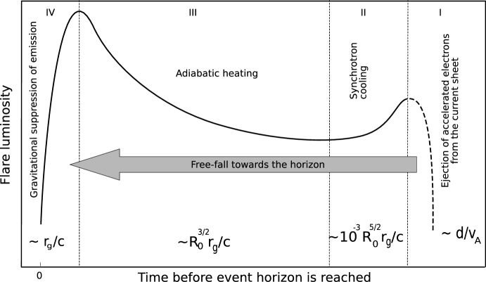
Figure 4: Internal structure of a flare as a reflection of the electron cloud evolution. The prevailing physical mechanisms defining the observed emission are denoted and typical durations of the stages are shown.

2 Search for isolated stellar mass black holes in optical range

As it has been already noted, the main indirect observational sign of the isolated stellar mass black hole is the absence of any spectral features in the emission of accreting plasma (except for interstellar absorption ones) (Shvartsman, 1971). Among such objects are the white dwarfs with featureless spectra (DC-dwarfs) and known localization (as they are usually selected as an objects with known proper motions) (McCook&Sion, 1999). On the other hand, in the last years by means of the cross-correlation of surveys of various wave bands (from radio to gamma) and the follow-up spectroscopic observations, the population of objects with featureless optical spectra and without known localizations, has been detected (Pustilnik, 1977; Tsarevsky et al, 2005). The latter include the radio objects with continuous optical spectra (ROCOSes) (Pustilnik, 1977). For them, as well as for some DC-dwarfs (Beskin&Mitronova, 1991), the upper limits on the fast optical variability as an observational manifestation of isolated stellar mass black holes have been derived for the first time (Shvartsman et al, 1989a, b). This idea became the basis of the observational programme for search for BH on Russian 6-m telescope - MANIA (Multichannel Analysis of Nanosecond Intensity Alterations) (Shvartsman, 1977; Beskin et al, 1997).

Recently, some evidences appeared that the isolated stellar mass black holes may be among the unidentified gamma-ray sources (Gehrels et al, 2000; La Palombara et al, 2004). The most promising cases are such where the independent estimation of the object mass is possible. One of such cases is the black hole in a binary system with a white dwarf. Such a binary may be detected by means of its periodic brightness amplification on the tens of seconds time scale due to gravitational microlensing (Beskin & Tuntsov, 2002). By using the technical equipment of SDSS (23^m limit in 6 square degree field) roughly 15 such objects may be detected in 5 years. It is clear that in such system it is easy to estimate the mass of the black hole, while there is no accretion from the white dwarf onto it, and the black hole interacts with the interstellar medium only. Another case when we may estimate the mass of the black hole are the long MACHO microlensing events (Bennett et al, 2002).

Below we present the results of observations of two candidates to the isolated stellar mass black holes.

3 Observations of objects-candidates to isolated stellar-mass black holes at 6-m telescope

Sample observations of the longest microlensing event MACHO 1999-BLG-22(Bennett et al, 2002), a most solid single stellar-mass black hole candidate, have been performed at the Special Astrophysical Observatory of RAS in 2003-2006 in the framework of the MANIA experiment(Beskin et al, 1997).

We used in observations the multichannel panoramic spectro-polarimeter (MPSP) based on position-sensitive detector (PSD) with 1 $\mu$s time resolution (Debur et al, 2003; Plokhotnichenko et al, 2003) (see Fig. 6). Such detectors use the set of multichannel plates (MCP) for electron multiplication, and multi-electrode collector to determine its position. PSD used in our observations has the following parameters: quantum efficiency of 10% in the 3700-7500 A range, (S20 photocathode), MCP stack gain of $10^{6}$, spatial resolution of 70 $\mu$m ($0.21^{\prime\prime}$ for the 6-m telescope), 700 ns time resolution, $7\cdot 10^{4}$ pixels with 22 mm working diameter, and the 200-500 counts/s detector noise. The acquisition system used is the “Quantochron 4-480” spectal time-code convertor with 30 ns time resolution and $10^{6}$ counts/s maximal count rate.

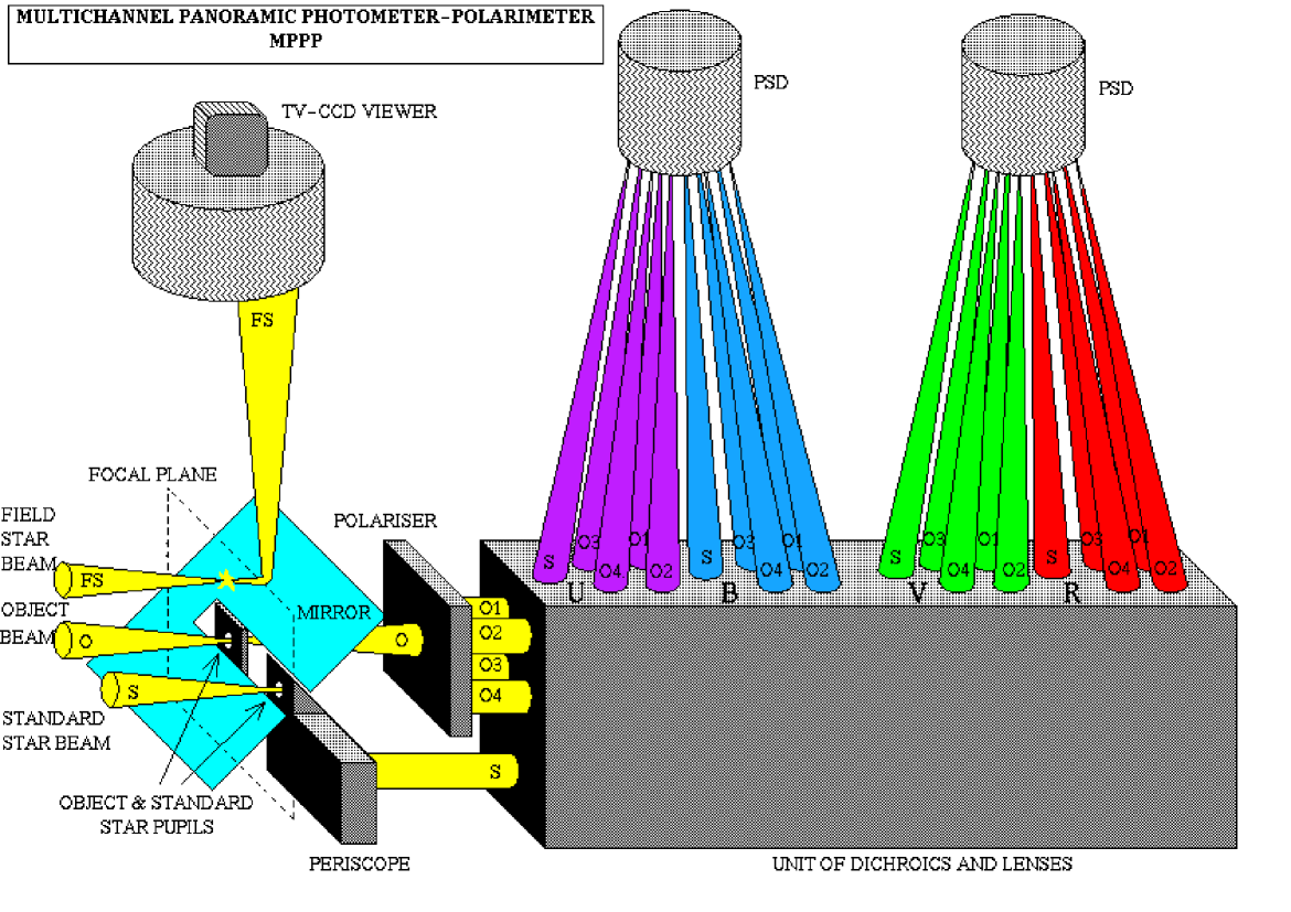
Figure 6: Optical scheme of the multichannel panoramic spectro-polarimeter (MPSP).

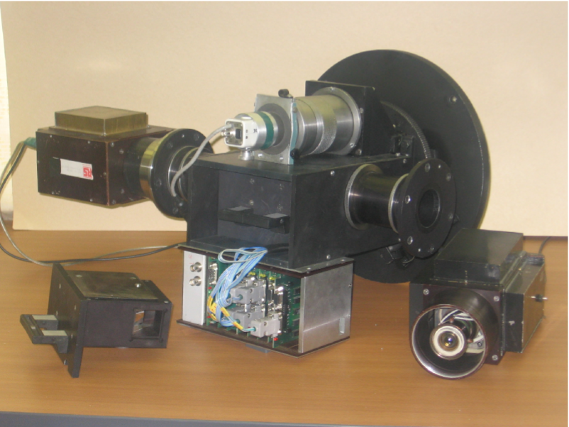
Figure 7: Multichannel panoramic spectro-polarimeter.

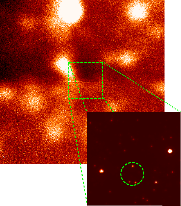
Figure 8: MACHO-1999-BLG-22, observed with panoramic photometer with high temporal resolution of Russian 6-m telescope. Overplotted is the Hubble ACS image with the blend resolved. Green circle is the position of the lens error box.

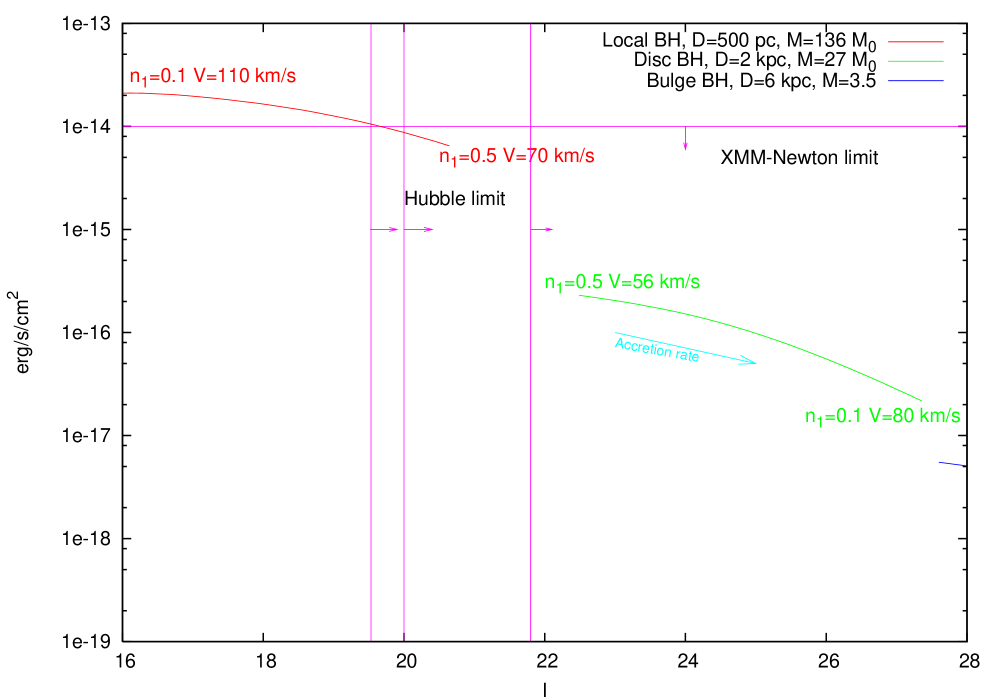
Figure 9: The prediction for the observational parameters of the MACHO-1999-BLG-22. The x-ray flux is in the 0.2-10 keV band. Overplotted are the limits from the XMM-Newton and Hubble ACS archival observations.

Figure 10: The optical Fourier power spectrum for the radio-loud x-ray source with featureless optical spectrum J1942+10. The upper limit for the variable emission component is 10% in $10^{-5}$ - 1 s range.

We combined our data with the archival observations of this region with XMM-Newton and Hubble ACS. We acquired the upper limits on the black hole x-ray emission on the level of $10^{-14}$ erg/s/cm².

The Hubble ACS optical data allow to de-blend the original source detected by (Bennett et al, 2002) on the level of $I=19.1^{\rm m}$. We performed the $I$-band photometry of the three stars of the blend and placed an upper limits of $I=19.5^{\rm m}$, $I=20.0^{\rm m}$ and $I=21.8^{\rm m}$ on the $I$-band emission of the BH for the three possible cases.

The parameters derived from the microlensing light curve don’t allow to get the unique value for the distance (and so, the mass) to the black hole. Instead, it points to the two possible configurations of the microlensing system, one with the lens at 500 pc (with $M=136M_{\odot}$) and the second with 2 kpc distance ($M=3.5M_{\odot}$). We also studied the intermediate case (2 kpc distance, $M=27M_{\odot}$).

The predicted observational parameters for these cases, computed according to our model, are shown in Fig. 9, with the observational limits overplotted.

Our results rule out the case of the near and massive black hole.

The analysis of data from 6-m telescope do not reveal any variable source. The upper limit on the variable emission component is placed on the $B=22^{\rm m}$ level for the $10^{-6}$ - 100 s time scale.

The J1942+10 is the radio-loud x-ray object with featureless optical spectrum with $B\sim 18^{\rm m}$. We observed it for 40 minutes in photometric mode and placed the upper limits on the B-band variability on the 10% level over the $10^{-5}$ - 1 s time scale (see Fig. 10).

4 Acknowledgements

This work has been supported by the Russian Foundation for Basic Research (grants No. 01-02-17857 and 04-02-17555), INTAS (grant No 04-78-7366), and by the grant of the Program ”Origin and Evolution of Stars and Galaxies” of the Presidium of RAS. S.K. thanks the Russian Science Support Foundation for support.

References

- Agol & Kamionkowski (2002) Agol, E., & Kamionkowski, M. “X-rays from isolated black holes in the Milky Way”, 2002, MNRAS, 334, 553-562
- Bennett et al (2002) Bennett, D.P. et al. “Gravitational Microlensing Events Due to Stellar-Mass Black Holes”, 2002, ApJ, 579, 639-659
- Beskin&Mitronova (1991) Beskin, G.M., & Mitronova, S.N. “The Revised Catalogue of DC Dwarfs - 1987”, 1991, Bulletin of the SAO RAS, 32, 33
- Beskin et al (1997) Beskin, G.M., et al. “The Investigation of Optical Variability on Time Scales of 10-10S: Hardware, Software, Results”, 1997, ExA, 7, 413-420
- Beskin & Tuntsov (2002) Beskin, G.M., & Tuntsov, A.V. “Detection of compact objects by means of gravitational lensing in binary systems”, A&A, 2002, 394, 489-503
- Beskin & Karpov (2005) Beskin, G.M., & Karpov, S.V. “Low-rate accretion onto isolated stellar-mass black holes”, A&A, 2005, 440, 223-238
- Beskin & Karpov (2006) Beskin, G.M., & Karpov, S.V., “Search for the event horizon evidences by means of optical observations with high temporal resolution”, Proceedings of the IAU Symposium 238 “Black Holes: from Stars to Galaxies”, edited by V.Karas & G.Matt. Cambridge University Press, in press
- Bisnovatyi-Kogan & Ruzmaikin (1974) Bisnovatyi-Kogan, G.S., & Ruzmaikin, A.A. “The Accretion of Matter by a Collapsing Star in the Presence of a Magnetic Field”, 1974, Ap& SS 28, 45
- Bisnovatyi-Kogan & Lovelace (1997) Bisnovatyi-Kogan, G.S., & Lovelace, R.V.E. “Influence of Ohmic Heating on Advection-dominated Accretion Flows”, 1997, ApJ, 486, L43
- Coppi (1999) Coppi, P.S., “The Physics of Hybrid Thermal/Non-Thermal Plasmas”, 1999, in “High Energy Processes in Accreting Black Holes”, ASP Conference Series 161, ed. Juri Poutanen & Roland Svensson, p.375
- Debur et al (2003) V. Debur, et al. “ Position-sensitive detector for the 6-m optical telescope”, Nuclear Instruments and Methods in Physics Research, 2003, A 513, 127-131
- Gehrels et al (2000) Gehrels, N., et al. “Discovery of a new population of high-energy gamma-ray sources in the Milky Way”, 2000, Nature, 404, 363-365
- Ipser & Price (1982) Ipser, J.R., & Price, R.H. “Synchrotron radiation from spherically accreting black holes”, 1982, ApJ, 255, 654-673
- La Palombara et al (2004) La Palombara, N., et al. “X-ray and optical coverage of 3EG J0616-3310 and 3EG J1249-8330”, MmSAI, 2004, 75, 476
- Lightman&Rybicki (1979) Lightman, A.P., & Rybicki, G.B. 1979, “Radiative Processes in Astrophysics”, 1986, published by Wiley-VCH. 1-400
- McCook&Sion (1999) McCook, G.P., Sion, E.M., “A Catalog of Spectroscopically Identified White Dwarfs”, ApJS, 1999, 121, 1-130
- Mii&Totani (2005) Mii, H., Totani, T., “Ultraluminous X-Ray Sources: Evidence for Very Efficient Formation of Population III Stars Contributing to the Cosmic Near-Infrared Background Excess?”, ApJ, 2005, 628, 2, 873-878
- Oppenheimer&Snyder (1939) Oppenheimer, J., & Snyder, H. 1939, Phys. Rev., 56, 455
- Paczynski (1991) Paczynski, B. “Gravitational microlensing of the Galactic bulge stars”, 1991, ApJ, 371, 63-67
- Plokhotnichenko et al (2003) Plokhotnichenko V. et al. “ The multicolor panoramic photometer-polarimeter with high time resolution based on the PSD”, 2003, Nuclear Instruments and Methods in Physics Research, A 513, 167-171
- Pustilnik (1977) Pustilnik, S.A. 1977, Soobsch. SAO, 18, 3
- Pustilnik (1997) Pustilnik, L.A. “Unsteady State of the Turbulent Current Sheet of a Flare”, 1997, ApSS, 252, 325-334
- Shapiro (1973) Shapiro, S.L. “Accretion onto Black Holes: the Emergent Radiation Spectrum”, 1973, ApJ, 180, 531-546
- Shvartsman (1971) Shvartsman, V.F. “Halos around black holes”, 1971, AZh, 48, 479-.
- Shvartsman (1977) Shvartsman, V.F. 1977, Soobsch. SAO, 19, 3
- Shvartsman et al (1989a) Shvartsman, V.F., Beskin, G.M., & Pustilnik, S.A. “The Results of Search for Superrapid Optical Variability of Radio Objects with Continuous Optical Spectra”, 1989a, Afz, 31, 457
- Shvartsman et al (1989b) Shvartsman, V.F., Beskin, G.M., & Mitronova, S.N. “A Search for 0.5-MICROSECOND to 40-SECOND Optical Variability in DC White Dwarfs”, 1989b, Astron. Report Letters, 15, 145
- Tsarevsky et al (2005) Tsarevsky, G, et al. “A search for very active stars in the Galaxy. First results”, A&A, 2005, 438, 949-955