Controlling Fano Profiles via Conical Intersections

Abstract

An ab initio analytical model for Fano resonances in two-channel systems is presented. We find that the lineshape parameter $q$ factors into a background contribution ${q_{\mathrm{b}}}$ that depends only on the uncoupled channels and an interaction contribution ${q_{\mathrm{i}}}$ that is affected by the coupling between the channels, revealing how the overall lineshape parameter $q$ may be controlled. In particular, we show how conical intersections of the background phase shifts have an important role in the interplay between ${q_{\mathrm{b}}}$ and ${q_{\mathrm{i}}}$. Finally, control of Fano transmission profiles through ${q_{\mathrm{b}}}$ and ${q_{\mathrm{i}}}$ is demonstrated for quantum billiards.

Fano resonances are ubiquitous whenever discrete levels interact with a continuum. They have been observed in many areas of physics: atomic and molecular systems Fano (1961); Cornett et al. (1999), quantum dots QDfano , carbon nanotubes Kim et al. (2003), and microwave billiards Rotter et al. (2005). When probed, Fano resonances yield their signature scattering cross-section profile Fano (1961)

$$\sigma\propto\frac{\left(\epsilon+q\right)^{2}}{1+\epsilon^{2}}\,,$$ (1)

which has been used as a fitting function for the results of many experiments as well as numerical calculations. Here $\epsilon$ is the dimensionless reduced energy (which is measured in units of the resonance’s half-width and shifted so that it vanishes at the position of the resonance), while $q$ is the Fano lineshape asymmetry parameter. The latter is proportional to the ratio between the resonant and non-resonant transition amplitudes Fano (1961). Unfortunately, this definition does not reveal any means of profile control. In this work we suggest how to manipulate the asymmetry parameter $q$ through a novel general analytical model for two-channels systems that can be specifically applied to two dimensional open quantum billiards (QBs).

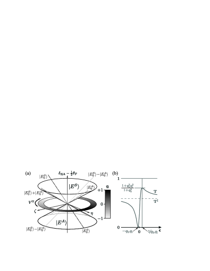
Figure 1: (a) Parameter space for controlling $q$ near a conical intersection of the background phase shifts. The upper cone corresponds to the state $|E^{S}\rangle$ and its phase shift $\delta_{S}$ (measured relative to $\mbox{$1\over 2$}\theta_{F}$). To leading order, this state is an azimuth-dependent linear combination of the vertex states $|E^{S\!/\!A}_{0}\rangle$. Changing the coupling $V^{\mathrm{II}}$ corresponds to rotating the ${q_{\mathrm{i}}}$ “compass wheel”. (b) The general form of the transmission Fano lineshape. The transmission zero is obtained at $\epsilon=-{q_{\mathrm{b}}}{q_{\mathrm{i}}}$, while the maximal transmission value $(1+{q_{\mathrm{b}}}^{2}{q_{\mathrm{i}}}^{2})/(1+{q_{\mathrm{b}}}^{2})$ is attained at $1/{q_{\mathrm{b}}}{q_{\mathrm{i}}}$. The transmission approaches the background value ${\bf T}^{\textrm{I}}$ as $|\epsilon|\to\infty$.

Our analysis reproduces the famous result of Eq. 1. However, the Fano lineshape parameter $q$ now factors as:

$$q={q_{\mathrm{b}}}\cdot{q_{\mathrm{i}}}.$$ (2)

Here ${q_{\mathrm{b}}}$ is responsible for the contribution of the uncoupled lower (background) channel, whereas ${q_{\mathrm{i}}}$ reflects the effect of the interaction between the two channels on the resulting profile. Our results show the crucial role played by the background transmission unity peaks, which correspond to conical intersections of the background phase shifts, see Fig. 1(a). The factor ${q_{\mathrm{b}}}$ corresponds to the radial distance from the vertex, and ${q_{\mathrm{i}}}$ behaves like the cosine of the azimuthal angle. Finally, the factorization opens the door to resonance profile control which we demonstrate for a quantum billiard model. This elucidates Fano $q$-reversals in a manner which is more complete and general than previous attempts Nakanishi et al. (2004).

Two-channel Model.— In order to analyze a multi-dimensional scattering process that yields a Fano profile, it is often useful to represent the system as a set (albeit infinite) of coupled channels. We assume a single-particle time-reversal invariant (TRI) multichannel system where only the lowest channel is open and the scattering energy is in the vicinity of an isolated bound state in the second channel, with other bound states energetically separate so that we may disregard them. The two-channel Hamiltonian is partitioned as $H=H^{0}+V^{\mathrm{I}}+V^{\mathrm{II}}$, so that the “distorted wave” formalism Taylor (1972), which treats scattering as a conceptual two-stage process, may be applied. The first scattering stage, with S-matrix $S^{\mathrm{I}}$, describes scattering due to $V^{\mathrm{I}}$ relative to the $H^{0}$ states in the first uncoupled channel. The potential $V^{\mathrm{I}}$ also accounts for the bound state $|\varphi\rangle$ at energy $E_{\varphi}$ in the second channel. The second scattering stage’s $S^{\mathrm{II}}$ describes the scattering of the $H^{0}+V^{\mathrm{I}}$ states under the influence of inter-channel interaction $V^{\mathrm{II}}$, which turns the bound state into a resonance. The scattering matrix for the entire two-stage process is $S=S^{\mathrm{I}}S^{\mathrm{II}}$ Taylor (1972); Berlatzky . In the present case it is assumed that $S^{\mathrm{I}}$ is known, and we shall show how $S^{\mathrm{II}}$ is approximated using the generic Fano model Fano (1961).

The first stage is a simple TRI 1D problem. Its S-matrix may be written as

$$S^{\mathrm{I}}=\begin{pmatrix}&t^{\phantom{-}}&&r^{-}\\ &r^{+}&&t^{\phantom{+}}\end{pmatrix}=\begin{pmatrix}&t^{\phantom{-}}&&re^{-i\delta_{r}}\\ &re^{+i\delta_{r}}&&t^{\phantom{+}}\end{pmatrix}\begin{matrix}\\ .\end{matrix}$$ (3)

This matrix has eigenvalues that satisfy $e^{2i\delta_{S}}=t+r$ and $e^{2i\delta_{A}}=t-r$, hence the notations $\delta_{{S\!/\!A}}$ refer to the symmetric/antisymmetric combinations of $t$ and $r$. The ambiguity in the above decomposition may be removed by one of the discrete gauge choices $-\pi/2<\delta_{r}\leq\pi/2$ or $\delta_{S}\geq\delta_{A}$. We also define the Friedel angle $\theta_{F}=\delta_{S}+\delta_{A}$ Friedel (1952), the difference $\Delta\theta=\delta_{S}-\delta_{A}$, and the states

$$|E^{S}\rangle =\frac{e^{-i\delta_{S}}}{\sqrt{2}}\left[e^{-\mbox{$i\over 2$}\delta_{r}}|E^{+}\rangle+e^{+\mbox{$i\over 2$}\delta_{r}}|E^{-}\rangle\right]$$ (4a)

$$|E^{A}\rangle =\frac{e^{-i\delta_{A}}}{i\sqrt{2}}\left[e^{-\mbox{$i\over 2$}\delta_{r}}|E^{+}\rangle-e^{+\mbox{$i\over 2$}\delta_{r}}|E^{-}\rangle\right]\!.$$ (4b)

where $|E^{\sigma}\rangle$ are the first stage scattering states at energy $E$ with incoming flux in the direction $\sigma=\pm$. These combinations are special in that they have real wavefunctions with the asymptotic boundary conditions $\langle x|E^{S}\rangle\sim\frac{1}{\sqrt{\pi k}}\cos(kx-\mbox{$1\over 2$}\delta_{r}\pm\delta_{S})$ and $\langle x|E^{A}\rangle\sim\frac{1}{\sqrt{\pi k}}\sin(kx-\mbox{$1\over 2$}\delta_{r}\pm\delta_{A})$ as $x\to\pm\infty$, where the kinetic energy is $\mbox{$1\over 2$}k^{2}$. These states are a generalization of the treatment for a Hamiltonian with parity symmetry Kahn (1961). The asymptotics also hold for unequal leads by using their respective wavenumbers. Time-reversal invariance implies that these states’ second stage coupling coefficients to the bound state $v_{E}^{{S\!/\!A}}=\langle\varphi|V^{\mathrm{II}}|E^{{S\!/\!A}}\rangle$ may be chosen to be real. Finally, the first-stage transmission coefficient is ${\bf T}^{\mathrm{I}}=\cos^{2}\big{(}\delta_{S}-\delta_{A}\big{)}$.

According to the Fano model Fano (1961), the first stage continuum is decomposed into states that couple to the bound state and those that don’t. The coupled states acquire the Fano phase shift $e^{2i\delta_{E}}$ due to the interaction with the bound state, where $\cot\left(\delta_{E}\right)=-2(E-E_{\varphi}-\Delta_{E})/\Gamma_{E}$, with the usual definitions $\Gamma_{E}=2\pi|v_{E}|^{2}$ and $\Delta_{E}=\frac{1}{2\pi}{\mathscr{P}}\int\!dE^{\prime}\,\frac{\Gamma_{E^{\prime}}}{E-E^{\prime}}$. Here $v_{E}$ is the radial coordinate of the point $(v_{E}^{S},v_{E}^{A})\in\mathbb{R}^{2}$, and we denote its angle as $\alpha$.

Finally, using these definitions, the total two-stage S-matrix is Berlatzky

$$S =S^{\mathrm{I}}S^{\mathrm{II}}=e^{i(\delta_{S}+\delta_{A}+\delta_{E})}\begin{pmatrix}\tau&&ie^{-i\delta_{r}}\rho^{-}\\ ie^{+i\delta_{r}}\rho^{+}&&\tau\end{pmatrix}\begin{matrix}\\ ,\end{matrix}$$ (5)

$$\tau =\cos^{2}\!\!\alpha\cos(\delta_{S}-\delta_{A}+\delta_{E})+\sin^{2}\!\!\alpha\cos(\delta_{S}-\delta_{A}-\delta_{E})$$

$$\rho^{\pm} =\cos^{2}\!\!\alpha\sin(\delta_{S}-\delta_{A}+\delta_{E})+\sin^{2}\!\!\alpha\sin(\delta_{S}-\delta_{A}-\delta_{E})$$

$$\pm 2i\sin\alpha\cos\alpha\sin\delta_{E}.$$

If $v_{E}$ varies slowly enough as a function of $E$ then it is reasonable to approximate $\Gamma_{E}$ and $\Delta_{E}$ using their values at the bound state’s energy $E_{\varphi}$ Cohen-Tannoudji et al. (1992). These are denoted as $\Gamma$ and $\Delta$. In addition, we assume a constant scattering background, i.e. $S^{\mathrm{I}}$ and its associated parameters are treated as constant, with values also taken at $E_{\varphi}$. This is a fair approximation when $\Gamma$ is much smaller than the scale for which $S^{\mathrm{I}}$ changes appreciably.

Next, let’s look at the Fano lineshapes. The ratio of the full two-stage transmission probability to that of the first stage assumes the almost familiar form

$$\frac{\ {\bf T}^{\phantom{\mathrm{I}}}}{\ {\bf T}^{\mathrm{I}}}=\frac{\big{(}\epsilon+{q_{\mathrm{b}}}{q_{\mathrm{i}}}\big{)}^{2}}{1+\epsilon^{2}},$$ (6)

with the usual reduced energy $\epsilon=-\cot\delta_{E}$ and the novel factorization of the lineshape parameter in Eq. 2 where

$${q_{\mathrm{b}}} =\tan\big{(}\delta_{S}-\delta_{A}\big{)}=\pm\sqrt{{\bf R}^{\mathrm{I}}/{\bf T}^{\mathrm{I}}}$$

$${q_{\mathrm{i}}} =\cos(2\alpha).$$

In these terms, the actual two-stage transmission coefficients is ${\bf T}=(\epsilon+{q_{\mathrm{b}}}{q_{\mathrm{i}}})^{2}/[(1+\epsilon^{2})(1+{q_{\mathrm{b}}}^{2})]$.

The general form of the transmission Fano lineshape is described in Fig. 1(b). Note that a symmetric lineshape is obtained not only when the background is zero (${q_{\mathrm{b}}}\to\pm\infty$ resulting in a Breit-Wigner Lorentzian) or unity (${q_{\mathrm{b}}}=0$ giving a symmetric Lorentzian dip), but also when ${q_{\mathrm{i}}}=0$. The latter occurs when the bound state is coupled with equal strength to $|E^{S}\rangle$ and $|E^{A}\rangle$.

Conical Intersections.— The lineshape asymmetry parameter $q$ factors into a background contribution ${q_{\mathrm{b}}}$ that solely depends on $V^{\mathrm{I}}$, and a coupling interaction contribution ${q_{\mathrm{i}}}$, which may be controlled using $V^{\mathrm{II}}$. However, neither ${q_{\mathrm{b}}}$ nor ${q_{\mathrm{i}}}$ are gauge invariant when taken alone, only their product is. This subtlety will be treated in detail in what follows. Understanding how $V^{\mathrm{II}}$ controls ${q_{\mathrm{i}}}$ is a simple affair — the decoupled first-stage surfaces $V^{\mathrm{I}}$ are not affected, so that ${q_{\mathrm{b}}}$ and the states $|E^{{S\!/\!A}}\rangle$ remain constant regardless of the specific gauge used to define them. On the other hand, modifying $V^{\mathrm{I}}$ may affect both ${q_{\mathrm{b}}}$ and ${q_{\mathrm{i}}}$, an effect that is predominant in the vicinity of background unity transmission peaks.

Suppose that at a scattering energy $E=E_{0}$ the background transmission reaches a unity peak, implying that $\delta_{S}^{0}=\delta_{A}^{0}$. Here we accent values at the transmission peak by a $0$ so that $S^{\mathrm{I}}_{0}=e^{i\theta_{F}^{0}}\mbox{1\hskip-2.5ptl}$. Assume throughout that $\delta_{S}$ approaches $\delta_{A}$ with a leading order linear in $E-E_{0}$. Since the background S-matrix is degenerate at this energy, there are no preferred eigenvectors. However, we may choose to use the states in Eqs. 4 that evolve smoothly from those obtained for values $E<E_{0}$, which we denote $|E^{{S\!/\!A}}_{0}\rangle$. These limiting states are associated with an angle $\delta_{r}^{0}$, which is just the limit of $\delta_{r}$ as $E_{0}$ is approached from below. Note that by a suitable choice of gauge (i.e. choosing which point to label $x=0$) it is possible to set $\delta_{r}^{0}=0$.

Now we modify $V^{\mathrm{I}}$ near the background transmission unity at $E_{0}$, leading to three types of infinitesimal deformations of the background S-matrix

$$dS^{\mathrm{I}}=iS^{\mathrm{I}}_{0}\left[\mbox{1\hskip-2.5ptl}d\xi+\Sigma_{r}^{0}\left(\sigma_{x}d\eta+\sigma_{y}d\zeta\right)\right],$$

where $\Sigma^{0}_{r}=\exp\big{(}-i\sigma_{z}\delta_{r}^{0}\big{)}$. Note the absence of a $\sigma_{z}$ generator which breaks TRI. The $\xi$ deformation affects only $\theta_{F}$, keeping the degeneracy intact, and it doesn’t change the eigenvectors, nor does it change the position of the transmission peak that still reaches unity. The $\eta$ deformation acts through the $\sigma_{x}$ generator. This removes the degeneracy, but to leading order $|E^{{S\!/\!A}}_{0}\rangle$ are still its eigenstates. It also shifts the position of the unity peak in the transmission spectrum away from $E_{0}$. Finally, the $\zeta$ deformations change the height of the peak whilst keeping its position. More importantly, $\zeta$-deformations are orthogonal to the $\eta$-deformations in the sense that the degeneracy is removed so that to leading order the eigenvectors are proportional to $|E^{S}_{0}\rangle\pm|E^{A}_{0}\rangle$.

The effect of these deformations on the first stage S-matrix may be described as a conical intersection of the phase shifts $\delta_{{S\!/\!A}}$ in the $\eta\zeta$-plane, schematically depicted in Fig. 1(a). Here the actual eigenstates $|E^{{S\!/\!A}}\rangle$ are defined according to the $\Delta\theta\geq 0$ gauge, i.e. $|E^{S}\rangle$ is on the upper cone. The leading order behavior of this state depends on the position in the parameter space. On one side of the $\eta$ axis $|E^{S}\rangle\sim|E^{S}_{0}\rangle$, while on the other it crosses over to $|E^{S}\rangle\sim|E^{A}_{0}\rangle$. Similarly, along the $\zeta$ axis it crosses over from $|E^{S}_{0}\rangle+|E^{A}_{0}\rangle$ to $|E^{S}_{0}\rangle-|E^{A}_{0}\rangle$.

One might naturally ask what topological phase is associated with these conical intersections. The answer is that $\delta_{r}$ shifts by $2\pi$ for each cycle that encircles a vertex, and this serves as the basis for adiabatic quantum swimming/pumping Avron et al. (2006).

The interplay between ${q_{\mathrm{b}}}$ and ${q_{\mathrm{i}}}$ can now be understood in terms of such conical intersections. The $\Delta\theta\geq 0$ gauge choice ensures that ${q_{\mathrm{b}}}>0$ on the conical surface (equaling zero at the vertex), so that up to appropriate parameterization dependent scale factors, ${q_{\mathrm{b}}}$ corresponds to the radial distance from the vertex in parameter space. In many cases it is also reasonable to assume that the bound state’s coupling to the $|E^{{S\!/\!A}}_{0}\rangle$ states remains (relatively) constant near the intersection. However, due to the behavior of $|E^{{S\!/\!A}}\rangle$ that changes according to the position in parameter space, the actual couplings to the bound state also change, so that ${q_{\mathrm{i}}}$ depends on the azimuthal angle’s cosine. The initial coupling to the $|E^{{S\!/\!A}}_{0}\rangle$ states may be modified through $V^{\mathrm{II}}$, and in effect this rotates the “compass wheel” in Fig. 1(a), i.e. ${q_{\mathrm{i}}}\equiv 1$ points in a different direction in the $\eta\zeta$-plane.

Quantum Billiard Example.— Recently, Fano resonances have been studied extensively in connection with QBs, see e.g. Rotter et al. (2005); Song et al. (2003). Usually, the QB is composed of an access lead from which the electrons impinge upon the main billiard, typically the part associated with a quantum dot, and an exit lead. The electron scattering problem in QBs can be cast into a one-dimensional coupled channel problem Klaiman et al. (2007); Berlatzky , where the channels are taken to be the energies of the modes in the transverse direction, and the inter-channel interactions are due to the non-adiabatic couplings Cederbaum (2004); Berlatzky .

Control of $q$ will be demonstrated on the QB depicted in Fig. 2(a). It consists of a rectangular cavity connected to leads that have two potential barriers of constant heights $V_{0}$, with widths $w^{{L\!/\!R}}$ and distances from the cavity $\ell^{{L\!/\!R}}$ that may be varied to modify $V^{\mathrm{I}}$. The latter’s first two adiabatic potential surfaces (channels) are depicted in Fig. 2(b). The leads may be offset by $\Delta^{{L\!/\!R}}$ in order to control the non-adiabatic couplings $V^{\mathrm{II}}$ resulting from the abrupt change in the local transverse basis at the cavity edges. Although the formalism detailed in Ref. Berlatzky, is used to calculate the actual non-adiabatic couplings, symmetry-based selection rules suffice for a qualitative understanding.

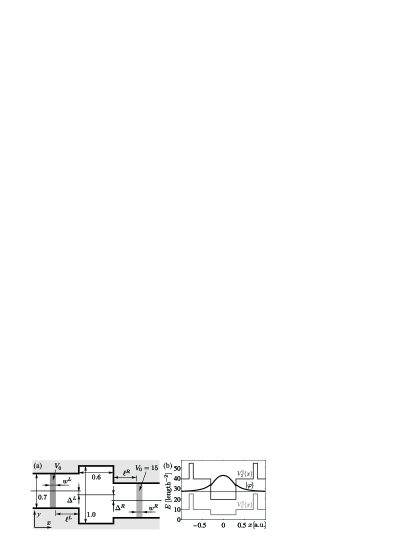
Figure 2: (a) Geometry of the quantum billiard with leads used to demonstrate control of Fano $q$-reversal. Length is measured in arbitrary units, while the energy scale is in units of [length^-2] (b) The first two adiabatic surfaces $V^{\mathrm{I}}_{1,2}(x)$ and the second surface bound state $|\varphi\rangle$.

The significance of a conical intersection is demonstrated near the unity transmission peak at $E_{0}=27.35$ for a parity symmetric $V^{\mathrm{I}}$ obtained by setting $w^{L\!/\!R}=0.1$ and $\ell^{L\!/\!R}=0.295$. This is convenient since the symmetry ensures that the states $|E^{S\!/\!A}_{0}\rangle$ have respective even and odd parity in the $\delta_{r}\equiv 0$ gauge. The background $V^{\mathrm{I}}$ is modified to control the lineshape parameter $q$ near the conical intersection. Taking $\Delta^{L\!/\!R}=0.01$ ensures that $V^{\mathrm{II}}$ couples $|\varphi\rangle$ exclusively to $|E^{S}_{0}\rangle$ by symmetry. We choose $\eta=\ell^{L}=\ell^{R}$, which preserves parity, and $\zeta$-deformations that break this symmetry.

Figure 3(a) depicts the Fano profiles resulting from the numerically exact multichannel calculation Sheng (1997), our analytical model, and the background contributions for several sets of parameters, see table. In all cases note the excellent fit between the actual multichannel calculations and the lineshapes predicted by our model. This series of calculations corresponds to two $q$-reversal paths in parameter space depicted in Fig. 3(b). The first path along the $\eta$ axis goes from point 1, with $q<0$, to 3 ($q>0$) by passing exactly through the background unity transmission peak at 2, where $q_{\mathrm{b}}=0$. Note that for point 1 the transmission peak’s energy has moved to the right of the resonance, while the opposite happens at point 3. The second path goes from 1 to 3 through $2^{\prime}$ which breaks parity symmetry. This point has a sub-unity background transmission peak, corresponding to a pure $\zeta$-deformation. As expected from the conical intersection, at this point in parameter space the states $|E^{S\!/\!A}\rangle$ are similar to $|E^{S}_{0}\rangle\pm|E^{S}_{A}\rangle$. This implies equal coupling to the bound state, so that ${q_{\mathrm{i}}}=0$, giving a symmetric dip with the novelty of a less than unity background.

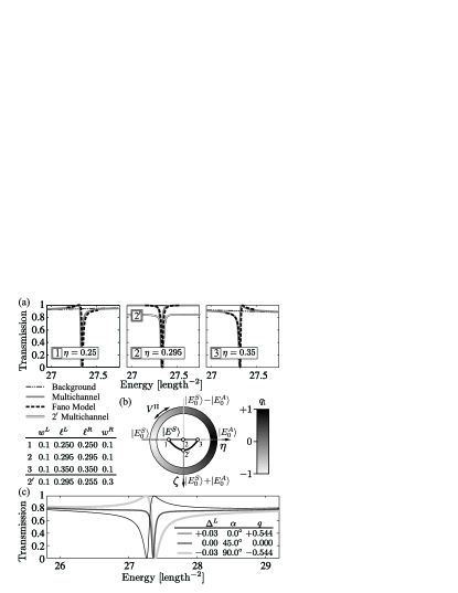
Figure 3: (a) Multichannel and analytical lineshapes obtained for various $V^{\mathrm{I}}$ parameters (see table). (b) These correspond to 2 paths in parameter space where $q$ reversal occurs. The overall lineshape parameter vanishes at the intermediate points: ${q_{\mathrm{b}}}=0$ at point 2 while ${q_{\mathrm{i}}}=0$ at $2^{\prime}$. (c) Variation of the non-adiabatic couplings $V^{\mathrm{II}}$, gives $q$-reversal due to the change in the coupling angle $\alpha$, and hence ${q_{\mathrm{i}}}$. The table summarizes analytical values calculated from the model.

Control of $q$ may also be affected through $V^{\mathrm{II}}$, which directly controls ${q_{\mathrm{i}}}$, whilst ${q_{\mathrm{b}}}>0$ remains constant. In the language of conical intersections the $V^{\mathrm{I}}$ parameters remain constant, so that $q$-reversal is achieved through a rotation of the “compass wheel”. This type of control works irrespective of the position in parameter space relative to conical intersections. For simplicity, again we choose a parity symmetric $V^{\mathrm{I}}$, this time with $\ell^{{L\!/\!R}}=0.4125$ and $w^{{L\!/\!R}}=0.1$ so that ${q_{\mathrm{b}}}=0.544$ throughout. Now we vary $\Delta^{L}=-0.03\mapsto 0.03$, while holding $\Delta^{R}=0.03$. The results of the numerically exact multichannel calculations are depicted in Fig. 3(c). The results are easily explained in terms of symmetry if we use the $\delta_{r}\equiv 0$ gauge. Since the second channel bound state has even parity, it is clear that for $\Delta^{L}=-0.03$ it couples exclusively to $|E^{A}\rangle$, while for $\Delta^{L}=+0.03$ it is coupled only to $|E^{S}\rangle$. Equal coupling, with $q_{i}=0$, is achieved for $\Delta^{L}=0.00$, yielding a sub-unity symmetric dip.

In summary, we have presented an analytical model for Fano resonances in coupled two-channel systems, where we found that the Fano lineshape parameter $q$ factors into background and interaction contributions. The model give accurate predictions for the actual transmission lineshapes. Moreover, it also provides insight to the relation between conical intersections of the background phase shifts, the coupling interaction, and the overall lineshape parameter $q$. This allows full control of $q$, which was demonstrated for a quantum billiard example.

The authors acknowledge useful discussions with N. H. Lindner and N. Moiseyev. This work was funded in part by the fund for promotion of research at the Technion.

References

- Fano (1961) U. Fano, Phys. Rev. 124, 1866 (1961).
- Cornett et al. (1999) S. T. Cornett et al., Phys. Rev. Lett. 82, 2488 (1999).
- (3) A. C. Johnson et al., Phys. Rev. Lett. 93, 106803 (2004); J. Gores et al., Phys. Rev. B 62, 2188 (2000); K. Kobayashi et al., Phys. Rev. Lett. 88, 256806 (2002).
- Kim et al. (2003) J. Kim et al., Phys. Rev. Lett. 90, 166403 (2003).
- Rotter et al. (2005) S. Rotter et al., Physica E 29, 325 (2005).
- Nakanishi et al. (2004) T. Nakanishi et al., Phys. Rev. B 69, 115307 (2004).
- Taylor (1972) J. R. Taylor, Scattering Theory (John Wiley & Sons, New York, 1972).
- (8) Y. Berlatzky, in preparation.
- Friedel (1952) J. Friedel, Philos. Mag. 43, 153 (1952).
- Kahn (1961) A. H. Kahn, Am. J. Phys. 29, 77 (1961).
- Cohen-Tannoudji et al. (1992) C. Cohen-Tannoudji, J. Dupont-Roc, and G. Grynberg, Atom-Photon Interactions: basic processes and applications (John Wiley & Sons, New York, 1992).
- Avron et al. (2006) J. E. Avron, B. Gutkin, and D. H. Oaknin, Phys. Rev. Lett. 96, 130602 (2006).
- Song et al. (2003) J. F. Song et al., Appl. Phys. Lett. 82, 4561 (2003); M. Mendoza et al. Phys. Rev. B 71, 245303 (2005).
- Klaiman et al. (2007) S. Klaiman, N. Moiseyev, and H. R. Sadeghpour, Phys. Rev. B 75, 113305 (2007).
- Cederbaum (2004) L. S. Cederbaum, in Conical Intersections, edited by W. Domcke, D. R. Yarkony, and H. Köppel (World Scientific, 2004).
- Sheng (1997) W.-D. Sheng, J. Phys.: Condens. Matter 9, 8369 (1997).