Non-minimally coupled multi-scalar black holes

Abstract

We study the static, spherically symmetric black hole solutions for a non-minimally coupled multi-scalar theory. We find numerical solutions for values of the scalar fields when a certain constraint on the maximal charge is satisfied. Beyond this constraint no black hole solutions exist. This constraint therefore corresponds to extremal solutions, however, this does not match the $\kappa=0$ constraint which typically indicates extremal solutions in other models. This implies that the set of extremal solutions have non-zero, finite and varying surface gravity. These solutions also violate the no-hair theorems for $N>1$ scalar fields and have previously been proven to be linearly stable.

arxiv:0709.2541

17 September 2007; LaTeX-ed

I Introduction

Black hole solutions with scalar fields are usually constrained to possessing only secondary hair by the “no-hair conjectures” Bekenstein:1971hc . Early attempts to find black hole solutions coupled solely to a scalar field found solutions where the scalar field diverged at the putative horizon Bekenstein:1974sf . Hence, technically such solutions cannot actually be considered black hole solutions due to a lack of a regular horizon. They are unlikely to have any physical relevance Sudarsky:1997te . The original “no-hair conjectures” have since been violated in a number of cases, either via coupling the scalar fields to both gravity and gauge fields, or through violation of the dominant energy condition. When the existence of scalar hair depends on a non-vanishing gauge field, and is entirely fixed by the mass, gauge charge and angular momentum this is called secondary hair Coleman:1991jf . In this paper we discuss a solution with contingent primary hair Mignemi:2004ms , that is to say the scalar hair depends on the existence of a non-vanishing gauge field but its behaviour is not entirely fixed by the values of the other asymptotic parameters. We briefly list some further “hairy” black hole solutions.

• Scalar fields coupled to higher order gravity have been heavily investigated since they arise naturally in low energy effective 4-dimensional string theories. The Gauss-Bonnet term, which is the only ghost-free leading order curvature correction, has naturally been of particular interest Mignemi:1992nt ; Chen:2006ge .

• Minimally coupled scalar fields with dominant energy condition violating potentials have been shown to allow non-trivial hair Bechmann:1995sa ; Dennhardt:1996cz ; Bronnikov:2001ah ; Nucamendi:1995ex . Examples have been found both analytically and numerically provided there is at least one global minimum with $V(\phi)<0$.

• Theories which couple gravity to non-Abelian gauge fields such as Einstein-Yang-Mills, Einstein-Yang-Mills-Higgs and Einstein-Skyrme, usually contain nonlinear self-interactions and admit “hairy” black holes. Einstein-Yang-Mills-Higgs and Einstein-Skyrme also include scalar fields. These vanish exponentially at infinity, however, and thus they do not have “Gauss-like’‘ scalar charge. These hairy black holes were thought to be generally unstable but it has been shown that some branches of solutions of the Einstein-Skyrme black holes are linearly stable Heusler:1992av . Whether they are non-linearly stable remains an open question.

• Scalar fields non-minimally coupled to an Abelian gauge theory have been shown to have hairy solutions Dobiasch:1981vh ; Gibbons:1985ac ; Gibbons:1987ps ; Garfinkle:1990qj . Such theories arise naturally in Kaluza-Klein theories and effective low-energy limits of string theory with a non-trivial dilaton.

Despite the solutions listed above being beyond the premises of the original “no-hair conjecture”, they are still considered interesting as tests of the limits of the conjectures. Stability is still an open problem in most cases.

For a non-rotating, static black hole with a single scalar field coupled to the $U(1)$ electromagnetic gauge field Gibbons:1987ps . This solution is not a member of the Reissner–Nordström class but is entirely specified by the values of M, Q and P. Adding an extra scalar field was shown to give more freedom Mignemi:1999zy and a version of scalar hair that falls between the definitions of primary and secondary hair. This was called contingent primary hair and has been generalised to $N$ scalar fields with linear stability being shown Mignemi:2004ms . Here we present numerical solutions to this model and discuss some of the features. As we will see, the most interesting feature is that these solutions limit to non-zero, finite surface gravity for an extremal black hole solution with a general coupling.

This paper is organised as follows. Section II discusses the model to be used and the analytical constraints that can be placed on the solutions. Section III contains the main results and gives details of the solutions found while the thermodynamic behaviour of these solutions is shown in section IV. We conclude with a discussion in section V. We use the notation of Mignemi:2004ms and define $c=4\pi\kappa^{2}=1$.

II Model

The general Lagrangian density for the $N$-scalar field case is

$${\cal{L}}=\frac{1}{4}\Bigg{[}R - 2\Lambda-2\sum^{N}_{i=1}\partial^{\mu}\Phi_{i}\partial_{\mu}\Phi_{i}$$ (1)

$$- \left({\sum^{N}_{i=1}\lambda_{i}^{2}}\right)^{-1}\sum^{N}_{i=1}\lambda_{i}^{2}e^{-2g_{i}\Phi_{i}}F_{\mu\nu}F^{\mu\nu}\Bigg{]},$$

where $R$ is the Ricci scalar and $F_{\mu\nu}$ is the electromagnetic field strength. Initially we consider the $N=2$ case with no cosmological constant, ie. $\Lambda=0$. For simplicity we split the representation of the scalar fields such that

$${\cal{L}}=\frac{1}{4}\Bigg{[}R - 2\partial^{\mu}\Phi\partial_{\mu}\Phi-2\partial^{\mu}\Psi\partial_{\mu}\Psi$$ (2)

$$- \frac{\lambda_{1}^{2}e^{-2g_{1}\Phi}+\lambda_{2}^{2}e^{-2g_{2}\Psi}}{\lambda_{1}^{2}+\lambda_{2}^{2}}F_{\mu\nu}F^{\mu\nu}\Bigg{]},$$

Since there is no potential dependent on any of the scalar fields, the Lagrangian density has the same scale invariance as the Gibbons-Maeda solution Gibbons:1987ps . This invariance applies under global re-scalings of the metric $g_{ab}\rightarrow\omega^{2}g_{ab}$ where $\nabla_{a}\omega=0$.

We use a standard metric ansatz for static, spherically symmetric Schwarzschild coordinates following the formalism of Nielsen:2005af .

$${\mathrm{d}}s^{2}=-A^{2}(r)\left(1-\frac{2m(r)}{r}\right){\mathrm{d}}t^{2}$$

$$+\frac{1}{1-\frac{2m(r)}{r}}{\mathrm{d}}r^{2}+r^{2}{\mathrm{d}}\Omega^{2}$$ (3)

where ${\mathrm{d}}\Omega^{2}={\mathrm{d}}\theta^{2}+\sin^{2}\theta{\mathrm{d}}\phi^{2}$ and $m(r)$ is the familiar Misner-Sharp mass function. In order for non-trivial solutions to exist we take the magnetic monopole field ansatz

$$F_{\theta\phi}=P\sin\theta$$ (4)

where $P$ is the magnetic charge. This choice is made out of convenience. Due to the scalar coupling to the electromagnetic sector, the electric ansatz includes dependence on the scalar fields and is therefore non-trivial, the magnetic ansatz, being the $\theta\phi$ components of the electromagnetic tensor, avoids these complications. There is no longer a simple duality between the magnetic and electric solutions although solutions for the electric solution should still be tractable if the magnetic solutions exist. We could, of course, also consider a situation where both are non-zero. As in the single scalar field of Gibbons:1987ps the scalar fields will necessarily vanish if $Q=P=0$.

The $G_{t}^{\hskip 2.84544ptt}$ component of the Einstein equations gives

$$\frac{2m^{\prime}}{r^{2}}=\Bigg{(}1 - \frac{2m(r)}{r}\Bigg{)}\left(\Phi^{\prime 2}+\Psi^{\prime 2}\right)$$ (5)

$$+ \left(\frac{\lambda_{1}^{2}e^{-2g_{1}\Phi}+\lambda_{2}^{2}e^{-2g_{2}\Psi}}{\lambda_{1}^{2}+\lambda_{2}^{2}}\right)\frac{P^{2}}{r^{4}}.$$

The linear combination $G_{t}^{\hskip 2.84544ptt}-G_{r}^{\hskip 2.84544ptr}$ of components of the Einstein equations gives

$$\frac{A^{\prime}}{A}=r\left(\Phi^{\prime 2}+\Psi^{\prime 2}\right),$$ (6)

while the two scalar field equations are

$$\partial_{r}\left(\left(1-\frac{2m(r)}{r}\right)Ar^{2}\partial_{r}\Phi\right)=-A\lambda_{1}^{2}g_{1}e^{-2g_{1}\Phi}\frac{P^{2}}{r^{2}}$$ (7)

and

$$\partial_{r}\left(\left(1-\frac{2m(r)}{r}\right)Ar^{2}\partial_{r}\Psi\right)=-A\lambda_{2}^{2}g_{2}e^{-2g_{2}\Psi}\frac{P^{2}}{r^{2}}.$$ (8)

We note these generalise to $N+2$ field equations for the system given in (1),

$$\frac{2m^{\prime}}{r^{2}}=\Bigg{(}1 - \frac{2m(r)}{r}\Bigg{)}\left(\sum^{N}_{i=1}\Phi_{i}^{\prime 2}\right)$$ (9)

$$+ \left(\sum_{i=1}^{N}\lambda_{i}^{2}\right)^{-1}\sum^{N}_{i=1}\lambda_{i}^{2}e^{-2g_{i}\Phi_{i}}\frac{P^{2}}{r^{4}}+\Lambda,$$

$$\frac{A^{\prime}}{A}=r\sum^{N}_{i=1}\Phi_{i}^{\prime 2}$$ (10)

and

$$\partial_{r}\left(\left(1-\frac{2m(r)}{r}\right)Ar^{2}\partial_{r}\Phi_{i}\right)=-A\lambda_{i}^{2}g_{i}e^{-2g_{i}\Phi_{i}}\frac{P^{2}}{r^{2}}.$$ (11)

III Numerical Solutions

Figure 1: Solution given by $\lambda_{1}=\lambda_{2}=g_{1}=g_{2}=1.0$, $P=0.5$ and with horizon values $m(r_{h})=0.25$, $\Phi(r_{h})=1.0$ and $\Psi(r_{h})=0.1$. $P_{\infty}=0.8611$ and $M_{ADM}=0.6674$ while $A(r_{h})=0.6490$ as found by the shooting method: (a) $m(r)$; (b) $A(r)$; (c) $\Phi(r)$; (d) $\Psi(r)$.

The $N=2$ solutions can be obtained numerically with the help of the following expansions near the horizon;

$$m(r) = m_{h}+m_{1}(r-r_{h})+m_{2}(r-r_{h})^{2}+...,$$

$$A(r) = A_{h}+A_{1}(r-r_{h})+A_{2}(r-r_{h})^{2}+...,$$

$$\Phi(r) = \Phi_{h}+\Phi_{1}(r-r_{h})+\Phi_{2}(r-r_{h})^{2}+...,$$

$$\Psi(r) = \Psi_{h}+\Psi_{1}(r-r_{h})+\Psi_{2}(r-r_{h})^{2}+....$$ (12)

In Fig. 1 we show the general form of the solutions for a non-extremal case.

The solution is uniquely defined by 3 asymptotic charges in the $N=2$ case and by $N+1$ charges in the general case. The Arnowitt, Deser and Misner (ADM) mass, $M_{ADM}$, is given by the asymptotic value of $m(r)$, while the asymptotic Gauss-like magnetic charge is given by

$$P_{\infty}=\sqrt{\frac{(\lambda^{2}_{1}e^{-2g_{1}\Phi_{\infty}}+\lambda_{2}^{2}e^{-2g_{2}\Psi_{\infty}})}{(\lambda_{1}^{2}+\lambda_{2}^{2})}}P.$$ (13)

These two asymptotic charges along with the coefficient $\Phi_{-1}$ of the $1/r$ term in the asymptotic $\Phi$ expansion

$$\Phi=\Phi_{\infty}+\frac{\Phi_{-1}}{r}+\frac{\Phi_{-2}}{r}+...,$$

uniquely define the solution. As shown in Mignemi:2004ms , $\Psi_{-1}$ is constrained in the $N=2$ case by

$$\Phi_{-1}^{2}+\Psi_{-1}^{2} + 2M_{ADM}\left(\frac{\Phi_{-1}}{g_{1}}+\frac{\Psi_{-1}}{g_{2}}\right)$$ (14)

$$- \left(\frac{\Phi_{-1}}{g_{1}}+\frac{\Psi_{-1}}{g_{2}}\right)^{2}=P_{\infty}^{2}.$$

and in general by

$$\sum^{N}_{i=1}\Phi_{-1,\,i}^{2}+2M_{ADM}\sum^{N}_{i=1}\frac{\Phi_{-1,\,i}}{g_{i}}-\left(\sum^{N}_{i=1}\frac{\Phi_{-1,\,i}}{g_{i}}\right)^{2}=P_{\infty}^{2},$$ (15)

where $\Phi_{-1,\,i}$ denotes the $1/r$ coefficient of the $i$th scalar field. This constraint limits the system to $N+1$ degrees of freedom, with these being in the magnetic monopole case, $M_{ADM}$, $P_{\infty}$ and {$\Phi_{-1,\,1}$, $\Phi_{-1,\,2}$,…,$\Phi_{-1,\,N-1}$}. The constraint, (15), holds throughout our numerical work to the numerical accuracies required.

We use the shooting method to find solutions such that

$$\lim_{r\rightarrow\infty}A=1,$$ (16)

where this condition is adhered to with a numerical accuracy of $10^{-7}$. This exploits the rescaling freedom in $A(r_{h})$ which can be seen in (6)-(8). This is a necessary requirement for the time coordinate $t$ in (II) to correspond to the proper time of static observers at infinity and gives the correct normalisation of the surface gravity. The numerical limits used to define the asymptotic region are $m^{\prime}(r)<10^{-8}$ and $r>500r_{h}$.

Figure 2: Behaviour of constraint given in (20) for $\lambda_{1}=\lambda_{2}=g_{1}=g_{2}=1.0$: (a) $P_{\infty}=1.2$; shows the solution approaching the limit as it reaches the extremal case at $M_{ADM}=0.849$ (numerical accuracy of $10^{-5}$ used for finding $P_{\infty}$ and $M_{ADM}$), note that although (a) shows the expected behaviour it does not allow comparison with the expected values for $\kappa=0$ as all quantities are defined at infinity; (b) $P=0.5$; approaches the limit $m(r_{h})=0.233$ while the required value for $\kappa=0$ from (19) is $m(r_{h})=0.173$.

We have also found solutions to both the $N=3$, $\Lambda=0$ and $N=2$, $\Lambda=-1$ cases. The $N=3$ case appear elsewhere leiththesis as there are no particular additional features when compared to the solutions in fig. 1. From these results, however, we would assume that solutions, with $N>2$ scalar fields, exist, having $N+1$ degrees of freedom. This may be of interest to string theory motivated work, where, in many cases a large or infinite number of scalar fields appear in the low energy effective 4-dimensional theory (see Douglas:2006es for a review).

The anti-de-Sitter (adS) solutions, while attainable, have distinct numerical issues related with finding solutions over a wide parameter range. However, the critical temperature generally exhibited by adS solutions, due to the thermal bath, may result in interesting behaviour when Hawking evaporation is considered if the unique thermodynamic features of the $N=2$, $\Lambda=0$ system shown below are also manifest in the $\Lambda=1$ case. This is left to further work although again solutions for a given parameter range appear in leiththesis .

IV Thermodynamic behaviour

The surface gravity for a black hole in these coordinates is given by Nielsen:2005af

$$\kappa=\frac{A(r_{h})}{4m(r_{h})}(1-2m^{\prime}(r_{h}))$$ (17)

Clearly we will have zero-temperature black hole solutions ($\kappa=0$) if $m^{\prime}(r_{h})=1/2$. In the horizon expansion given above this would correspond to $m_{1}=1/2$ while from the equation of motion (5) we find

$$m_{1}=\frac{P^{2}}{2r^{2}}\left(\frac{\lambda_{1}^{2}e^{-2g_{1}\Phi_{h}}+\lambda_{2}^{2}e^{-2g_{2}\Psi_{h}}}{\lambda_{1}^{2}+\lambda_{2}^{2}}\right).$$ (18)

Hence, $\kappa=0$ when

$$m(r_{h})\Big{|}_{\kappa=0}=\frac{P}{2}\sqrt{\frac{\lambda_{1}^{2}e^{-2g_{1}\Phi_{h}}+\lambda_{2}^{2}e^{-2g_{2}\Psi_{h}}}{\lambda_{1}^{2}+\lambda_{2}^{2}}},$$ (19)

where we have used $r_{h}=2m(r_{h})$. We have denoted this limiting case as $m(r_{h})|_{\kappa=0}$ as it turns out not to be the extremal case. The “extremal solution” is the solution existing with the maximum electromagnetic charge for a given mass and scalar charge.

We find that the separate condition given in Mignemi and Wiltshire Mignemi:2004ms ,

$$P_{\infty}^{2}\leq M_{ADM}^{2}+\sum^{N}_{i=1}\Phi_{-1,\,i}^{2},$$ (20)

is the constraint for extremal black holes. This constraint has no thermodynamic significance but the equality indicates the degenerate horizon. This is a novel situation as when (19) and (20) are considered we find $P_{\infty,extremal}<P_{\infty,\kappa=0}$. For the degenerate horizon, given by the equality in (20), we find that the horizon becomes singular and hence does not have a well-defined surface gravity. This is indicated by divergence of the coefficient $m_{1}$ in (12).

The limiting cases, however, still indicate extremal black hole solutions with non-zero, finite surface gravity for general couplings, $g_{i}$. Such results have been found previously for specific couplings Gibbons:1987ps .

The limiting behaviour due to (20) is shown in fig. 2, where $\Phi_{-1}$ is defined by

$$\Phi_{-1}=g_{1}\lambda_{1}^{2}P^{2}\int^{\infty}_{r_{h}}\frac{e^{-2g_{1}\Phi}}{r^{2}}A{\mathrm{d}}r,$$ (21)

and similarly for $\Psi_{-1}$ Mignemi:2004ms .

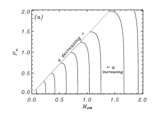
Figure 3: Contour plots showing the behaviour of the surface gravity; $\lambda_{1}=\lambda_{2}=1.0$ with horizon values $\Phi(r_{h})=1.0$ and $\Psi(r_{h})=0.1$: (a) $g_{1}=g_{2}=1.0$; (b) $g_{1}=g_{2}=3.0$. Note the change in behaviour from Reissner-Nordström-like solutions in (a) where the specific heat changes sign for $P_{\infty}=const$ as it moves away from the extremal limit while in (b) the specific heat for $P_{\infty}=const$ is always negative and mimics the well-known Kaluza-Klein examples. The extremal limit is shown as a dotted line as it is not an ‘isotherm’, instead the surface gravity decreases with increasing $P_{\infty}$.

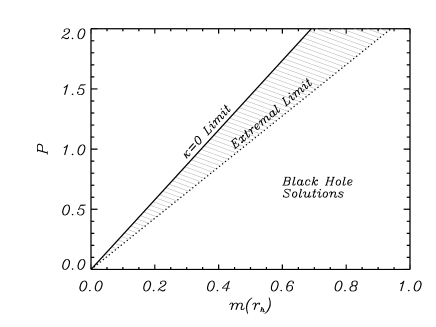
Figure 4: The dotted line shows the constraint (20) while the solid line indicates the limit imposed by (19) for $\lambda_{1}=\lambda_{2}=g_{1}=g_{2}=1.0$, $\Phi(r_{h})=1.0$ and $\Psi(r_{h})=0.1$ while varying over horizon values for $m(r_{h})$ and the ‘bare’ $P$ values.

Contour plots of the surface gravity show Reissner-Nordström-like solutions when $g_{1}=g_{2}=1.0$ and Kaluza-Klein-like solutions when $g_{1}=g_{2}=3.0$ see Fig. 3(a) and Fig. 3(b) respectively. The ‘specific heat’, defined as $C\equiv(\partial M_{ADM}/\partial T)|_{P_{\infty}}\sim(\partial M_{ADM}/\partial\kappa)|_{P_{\infty}}$, changes sign in fig. 3(a) while it is always negative for fig. 3(b). Unfortunately we do not possess the computational power to find the limit of the coupling gradients that produce these two types of solutions.

The extremal limit in these cases is not an ‘isotherm’ but instead tends to finite non-zero values where the surface gravity is decreasing with increasing $P_{\infty}$. The contours mimic those found in Gibbons:1987ps but with a region excluded due to the constraint (20). Fig. 4 shows this graphically. However, we would caution that the extremal solution falls into a different class from those solved by the numerical method implemented here. As the value of $m^{\prime}(r_{h})$ diverges we do not have well-defined solutions and hence no surface gravity. We therefore only comment on the limiting behaviour for the extremal cases.

V Discussion

We have numerically demonstrated linearly stable black hole solutions with contingent primary hair. The condition (15), as previously derived in Mignemi:2004ms , gives $N+1$ asymptotic charges for $N$ scalar fields with two being $M_{ADM}$ and $P_{\infty}$ (in the non-zero magnetic monopole solution considered here) with the other $N-1$ charges being the $1/r$ coefficients of the asymptotic expansion of $N-1$ of the scalar fields, {$\Phi_{-1,1}$,$\Phi_{-1,2}$,…,$\Phi_{-1,N-1}$}. This violation of the no-hair theorems is, however, not entirely within the confines of the premise under which the theorems were originally derived as we have non-minimal coupling between the scalar field and the $U(1)$ gauge field.

The solutions here may help to shed some light on black hole solutions to the low energy effective 4-dimensional string theory when coupled with further corrections, such as, higher-order gravity terms Chen:2006ge , another $U(1)$ field or the inclusion of scalar potentials. Chen et al. have found constraints on the value of the coupling in the single scalar case when a Gauss-Bonnet term is introduced. This appears to limit the applicability in string theory motivated situations. However, this constraint would possibly be weakened by additional scalar fields, similar to the case for the slope of the potential when additional scalar fields are considered in cosmology Liddle:1998jc .

The result of major interest is that the solutions are bounded by (20) and do not contain the $\kappa=0$ case. At the extremal limit no surface gravity is defined, it does, however, limit to finite, non-zero values. Previously this behaviour has only been seen in Gibbons:1987ps when considering the limiting case between Reissner-Nordström and Kaluza-Klein type solutions for a single scalar field with $g=\sqrt{D-1}$. Although (15) limits the number of independent asymptotic charges, it does not allow us further insight into the nature of the horizon. The Gibbons-Maeda solution allowed analysis of the horizon in the extremal case, indicating a singularity. This would seem likely in the present case as $m^{\prime}(r)$ diverges at the horizon indicating a curvature singularity.

References

- (1) J. D. Bekenstein, Phys. Rev. D 5, 1239 (1972); Phys. Rev. D 5, 2403 (1972).
- (2) J. E. Chase, Comm. Math. Phys. 19, 276 (1970); J. D. Bekenstein, Annals Phys. 82, 535 (1974); Annals Phys. 91, 75 (1975).
- (3) D. Sudarsky and T. Zannias, Phys. Rev. D 58, 087502 (1998) [arXiv:gr-qc/9712083].
- (4) S. R. Coleman, J. Preskill and F. Wilczek, Phys. Rev. Lett. 67, 1975 (1991); Nucl. Phys. B 378, 175 (1992) [arXiv:hep-th/9201059]; A. D. Shapere, S. Trivedi and F. Wilczek, Mod. Phys. Lett. A 6, 2677 (1991).
- (5) S. Mignemi and D. L. Wiltshire, Phys. Rev. D 70, 124012 (2004) [arXiv:hep-th/0408215].
- (6) M. Heusler, S. Droz and N. Straumann, Phys. Lett. B 285, 21 (1992).
- (7) S. Mignemi and N. R. Stewart, Phys. Rev. D 47, 5259 (1993) [arXiv:hep-th/9212146].
- (8) C. M. Chen, D. V. Gal’tsov and D. G. Orlov, Phys. Rev. D 75, 084030 (2007) [arXiv:hep-th/0701004].
- (9) O. Bechmann and O. Lechtenfeld, Class. Quant. Grav. 12, 1473 (1995) [arXiv:gr-qc/9502011].
- (10) H. Dennhardt and O. Lechtenfeld, Int. J. Mod. Phys. A 13, 741 (1998) [arXiv:gr-qc/9612062].
- (11) K. A. Bronnikov and G. N. Shikin, Grav. Cosmol. 8, 107 (2002) [arXiv:gr-qc/0109027].
- (12) U. Nucamendi and M. Salgado, Phys. Rev. D 68, 044026 (2003) [arXiv:gr-qc/0301062].
- (13) P. Dobiasch and D. Maison, Gen. Rel. Grav. 14, 231 (1982).
- (14) G. W. Gibbons and D. L. Wiltshire, Annals Phys. 167, 201 (1986) [Erratum-ibid. 176, 393 (1987)].
- (15) G. W. Gibbons and K. i. Maeda, Nucl. Phys. B 298, 741 (1988).
- (16) D. Garfinkle, G. T. Horowitz and A. Strominger, Phys. Rev. D 43, 3140 (1991) [Erratum-ibid. D 45, 3888 (1992)].
- (17) S. Mignemi, Phys. Rev. D 62, 024014 (2000) [arXiv:gr-qc/9910041].
- (18) A. B. Nielsen and M. Visser, Class. Quant. Grav. 23, 4637 (2006) [arXiv:gr-qc/0510083].
- (19) Ben. M. Leith, Ph.D thesis, University of Canterbury, (2007).
- (20) M. R. Douglas and S. Kachru, Rev. Mod. Phys. 79, 733 (2007) [arXiv:hep-th/0610102].
- (21) A. R. Liddle, A. Mazumdar and F. E. Schunck, Phys. Rev. D 58, 061301 (1998) [arXiv:astro-ph/9804177].