A Photometric Search for Transients in Galaxy Clusters

Abstract

We have begun a program to search for supernovae and other transients in the fields of galaxy clusters with the 2.3m Bok Telescope on Kitt Peak. We present our automated photometric methods for data reduction, efficiency characterization, and initial spectroscopy. With this program, we aim to ultimately identify $\sim$25-35 cluster SN Ia ($\sim$10 of which will be intracluster, hostless events) and constrain the SN Ia rate associated with old, passive stellar populations. With these measurements we will constrain the relative contribution of hostless and hosted SN Ia to the metal enrichment of the intracluster medium. In the current work, we have identified a central excess of transient events within $1.25r_{200}$ in our cluster fields after statistically subtracting out the ’background’ transient rate taken from an off-cluster CCD chip. Based on the published rate of SN Ia for cluster populations we estimate that $\sim$20 percent of the excess cluster transients are due to cluster SN Ia, a comparable fraction to core collapse (CC) supernovae and the remaining are likely to be active galactic nuclei. Interestingly, we have identified three intracluster SN candidates, all of which lay beyond $R>r_{200}$. These events, if truly associated with the cluster, indicate a large deficit of intracluster (IC) SN at smaller radii, and may be associated with the IC stars of infalling groups or indicate that the intracluster light (ICL) in the cluster outskirts is actively forming stars which contribute CC SN or prompt SN Ia.

1. Introduction

Because little can escape the deep gravitational potential wells of galaxy clusters, they are among the only sites where one can confidently construct constrained models of chemical enrichment. The intracluster medium (ICM) contains most of the baryons in clusters (e.g., Gonzalez et al. 2007) and is metal enriched, $\langle Fe/H\rangle\sim 0.3Z_{\odot}$ (e.g., Balestra et al. 2007). However, none of the proposed mechanisms to transport the metals produced by supernovae from the galaxies in which they lie to the ICM have proven adequate — unless large gas outflows from cluster members are invoked (Renzini 1997, see also discussion in Dupke & White 2000). We are left to conclude either that galaxies somehow eject most of their metals, some basic part of the chemical evolution model, such as the SNe rate or yield, is incorrect, or an enrichment channel has been overlooked.

One such channel that has recently been proposed is enrichment by intracluster stars (ICS) whose SNe pollute the ICM in situ (Sasaki 2001; Zaritsky et al. 2004; Domainko et al. 2004; Lin & Mohr 2004; Sivanandam et al. 2007). Because the ICS comprise $\sim$30% of the total cluster stellar budget (Gonzalez et al. 2005, 2007), a comparable fraction of the ICM metals should come from this population even if galactic winds are highly efficient. A quantitative attempt to determine whether the dominant source of metals is the ICS or the cluster galaxies has been unable to distinguish between the two sources because of uncertainties in cluster SNe rates and SN Ia progenitors (Sivanandam et al. 2007).

Despite the widespread use of SNe Ia’s as a probe of the cosmic expansion history, the progenitor systems of SNe Ia remain unidentified (e.g., Hillebrandt & Niemeyer 2000). Understanding the origins and basic physics behind SNe Ia is essential, given that their use as standard candles rests on the assumption that their basic properties are constant as a function of cosmic time and that their luminosities can be calibrated with an unchanging empirical relation (see recent review by Filippenko 2005). One interpretation of the shortfall of metals in the chemical evolutionary models is that there exists a population of SNe that we are missing. Because we do not understand the origin of Ia’s, this possibility must be considered.

Independent recent results indeed suggest that SN Ia come from two different stellar populations (Mannucci et al. 2005; Scannapieco & Bildsten 2005; Sullivan et al. 2006). One type is associated with star forming regions, which tend to be overluminous, have a rate proportional to the star formation rate, and appear within 1 Gyr of the formation of the stellar population. The other type is associated with old stellar populations, have a rate that is proportional to the total stellar mass of the system, and only appear many Gyrs after the formation of the stellar population. A SN search that probes both young and old stellar populations must use the star formation history of the survey volume to disentangle the two SNe Ia populations (e.g., Sullivan et al. 2006) and measure the SN rate for each population. This necessary modeling leads to larger uncertainties in the inferred rates.

Old, elliptical galaxies only give rise to SN Ia associated with the long delay time population (Sullivan et al. 2006), which makes galaxy clusters the natural environment in which to constrain the rate of this type of SNe Ia. By pursuing a SN survey in low redshift galaxy clusters the modeling problem is averted because old stellar populations dominate. The star formation history of these galaxies can be approximated to high accuracy as a star formation burst at high redshift (e.g., Holden et al. 2005). Furthermore, the profusion of old ellipticals in clusters also makes it possible to measure the rate of these SNe even though the rate is quite low.

There have been several modern SN surveys that have focused on the galaxy cluster environment, beginning with that of Norgaard-Nielsen et al. (1989). The first systematic survey, the Mount Stromlo Abell Cluster Supernova Search (Reiss et al. 1998), ran for 3.5 years and discovered 52 SNe, 25 of which were associated with the cluster targets. The survey focused on Abell clusters at $0.02<z<0.08$, and of the 25 cluster SN Ia, 14 were confidently determined to be SN Ia. This survey did not attempt a SN Ia rate measurement. Gal-Yam et al. (2002) searched Hubble Space Telescope archival images of nine galaxy clusters that had more than one imaging epoch for SNe. Despite finding only two probable cluster SN, they were able to put the first real limits on the SNe rate in clusters at both low and high redshift. This same group has undertaken a longer term program in low redshift ($0.06<z<0.19$) galaxy clusters, as part of the Wise Observatory Optical Transient Search (WOOTS; Gal-Yam et al. 2007). Their results include the discovery of two IC SN Ia (Gal-Yam et al. 2003) and a measurement of the SN Ia rate in galaxy clusters based on six SN Ia (Sharon et al. 2007b). Very recently, Mannucci et al. (2007) presented a measurement of both the SN Ia and CC SN rate in local galaxy clusters, measuring the cluster SN Ia rate to be $\sim$3 times higher than that in field E/S0 galaxies. Work has also begun at higher redshift (Sharon et al. 2007a).

Motivated by all of the above, we began a long-term photometric monitoring campaign of $\sim$60 X-ray selected galaxy clusters at $0.1<z<0.2$ using the 2.3 m Bok telescope on Kitt Peak with its 90Prime 1-degree field imager (Williams et al. 2004). We aim to measure the old-population, SN Ia rate, both in cluster galaxies and among the ICS. The data are also being used to study other transient phenomena. Here, we present the observational design of the survey, transient detection techniques and efficiency calculations, initial spectroscopy and first science results. In § 2, we describe the cluster sample, survey design and scientific goals. In § 3 we discuss our automated image reduction pipeline and transient detection technique, followed by our calculated transient detection efficiency in § 4. We present our current transient catalog in § 5, along with a sample of transients that do not appear to lie within galaxies, which are generally referred to as hostless. Our initial spectroscopy is presented in § 6. We present evidence for a central overdensity of transient sources associated with our cluster sample in § 7 and discuss the nature of these sources in § 8. We devote § 9 to a discussion of the intriguing implications of the three IC SN candidates at $R>r_{200}$. Finally, in § 10 we outline our future plans. Where necessary, we adopt a flat cosmology with $H_{0}$=70 km $\textrm{s}^{-1}$Mpc^-1, $\Omega_{m}$=0.3, and $\Omega_{\Lambda}$=0.7.

2. Survey Design and Goals

The basic observational goal of this survey is to confidently identify SNe Ia within the galaxy clusters in our sample at $0.1<z<0.2$, whether they lie among the ICS (hostless) or within cluster galaxies (hosted). Given our observational strategy and depth, we will eventually correct the observed SN rate to the true rate, measure whether there are significant differences among the hosted and hostless events, and ultimately improve the model of the metal enrichment history of the ICM.

Various considerations play a role in the survey design, including the available field of view, image depth, survey cadence, and sample size. From the depth we achieve with modest exposure times (total 1600 sec, see below), and a desire to have control fields near the clusters, we decided to constrain the sample to redshifts between 0.1 and 0.2. As described in more detail below, we roughly center our clusters on CCD chip 1 of 90Prime, the prime focus wide field imager on the 2.3m Bok telescope on Kitt Peak. We use the other three chips to measure the background transient detection rate, given that there is a $\sim$500 arcsecond gap between them. The $\sim$30’ x 30’ field of chip 1 corresponds to a radius of $\sim$1.6 Mpc at z=0.1 and $\sim$3.0 Mpc at z=0.2 and allows us to probe out beyond $r_{200}$ in all of our clusters.

The peak magnitude of type Ia supernovae is $M_{B}=-19.25$, with a small intrinsic dispersion of $0.2-0.3$ mag (Phillips 1993). For the redshift range of our cluster sample, this corresponds roughly to $19<g<20$ mag. Type Ia SNe fade by $\sim$ 1 mag in 15 rest frame days. By taking four 400 second $g$ band exposures with small dithers we easily find SN candidates down to $g\sim 21.5$ during good observing conditions (see § 4), allowing us to observe SNe Ia’s well before and after peak brightness. We will present our formal effective visibility time, the time during which a given survey image is sensitive to SNe, in future work as we determine the SNe Ia rate in our cluster sample. We present preliminary calculations in § 8.1.

For an exposure time of 4$\times$400 seconds per cluster field and a generous allocation of $\sim$4 nights per month on the 2.3m Bok telescope (excluding the southern Arizona monsoon season), we can survey about 60 galaxy clusters monthly. In addition to spectroscopic followup of a fraction of our cluster SNe candidates, we are also experimenting with multi-band imaging of each cluster field at each epoch to exploit recent progress in single-epoch phototyping of supernovae candidates (Poznanski et al. 2006), but do not describe the latter here. We also employ other methods for statistical determinations of the rate of cluster transients (see § 10).

As will be discussed in § 8.1, we expect to find $\sim$2-3 cluster SN Ia per month of 90Prime imaging employing the above strategy. If the program runs for two observing seasons, each spanning six months, we will discover $\sim$25-35 cluster SN Ia, with between $\sim$5 and 10 of these being hostless, IC events. This survey, when completed, will have 4-6 times the number of cluster SN Ia than previous focused searches which have sought to measure the rate in clusters. Overcoming previous surveys’ small number statistics is essential for pinning down the rate and understanding the long-delay time SN Ia population.

Several secondary science goals can also be pursued with these data. For example, active galactic nuclei (AGN) and quasi-stellar objects (QSOs) constitute a large fraction of our transient objects (see § 5 and 6). Identification of AGN/QSOs through their variability is highly complementary to other AGN selection techniques (Sarajedini et al. 2003, 2006; Totani et al. 2005), and may be useful in cluster fields where there is a known overdensity of AGN (Ruderman & Ebeling 2005; Martini et al. 2007). Another example is the use of our 4$\times$400 second image sequence to study short time scale variability (e.g., Becker et al. 2004). A final example is the study of rare, mysterious transient events in cluster cores such as that identified in Abell 267 which at the time could not be fit by any known supernova template (Stern et al. 2004).

2.1. Sample Selection

We chose our cluster sample from among $0.1<z<0.2$ X-ray selected galaxy clusters visible from northern hemisphere telescopes with a preference for galaxy clusters with known strong lensing features (to increase our chances, albeit low, of discovering strongly lensed transient phenomena). Clusters were preferably chosen to have a high X-ray luminosity, although not in any systematic way. The cluster sample, along with the observing epochs included here, is detailed in Table 1. The X-ray luminosities are those reported directly from the BAX online cluster data base, which attempts to homogenize luminosities based on flux measurements and uses a $H_{0}$=50 km $\textrm{s}^{-1}$Mpc^-1 and $\Omega_{m}$=1.0 cosmology. We refer the reader to the BAX web site for details.

3. Photometric Transient Search

The observations were conducted with the prime focus imager, 90Prime (Williams et al. 2004), on the 2.3m Bok telescope on Kitt Peak. The focal plane array consists of a mosaic of four Lockheed 4k $\times$ 4k blue sensitive CCDs (the peak QE is near 4500 Å). With the pixel scale of $0\farcs 45$ per pixel, this detector array gives a field of view of about one square degree. The chip gaps are large, approximately 500 arcseconds on the sky. For our purposes, these gaps are actually an advantage because it places the other chips farther away from the cluster. We center our cluster fields on Chip 1 (cosmetically the best out of the four), giving coverage out to at least $r_{200}$ for all targets. The other three chips provide control fields. Here, we present transients from chip 3, in addition to chip 1, to quantify the background transient rate. A charge trap in chip 3 decreases the effective field of view by approximately one-eighth, but otherwise the chip is relatively free of defects.

The images considered here were obtained between January and June 2006, during four observing runs (our pilot program), and one night in December 2006. The single December night was followed by one night of spectroscopy, which we present in § 6. Several other runs beyond the pilot program, which implemented this imaging plus spectroscopy strategy, were spoiled either due to weather or instrument problems, leaving only the one useable night in December 2006 where everything worked. There are five clusters (noted in Table 1) whose only additional epoch of imaging were taken during the period of the Fall 2006 campaign when the 90Prime imager was operating with anomalously high readout noise. Since these images are of lower quality, they are not generally included in this study, but are used only as the reference image for differencing of the good December data in these five clusters.

3.1. Basic Image Calibration

The image processing consists of various steps that we describe here. We do the initial image reductions using a nearly automated IRAF script that relies heavily on the mscred mosaic data reduction system. This script corrects for cross talk, trims and subtracts the overscan region, applies an additional bias subtraction to remove structure seen in the bias exposures, flat-fields the data and rejects cosmic rays in each individual exposure using the LACOSMIC task (van Dokkum 2001). Regions around saturated and nearly-saturated objects are heavily masked because residuals near poorly subtracted bright objects can be one of the largest sources of false detections in our transient detection pipeline. We calculate exposure weight maps using a combination of a normalized twilight flat field and the cosmic ray rejection map. We edit each image header to include the refined world coordinate system solution obtained using the msccmatch task and the USNO-A2 catalog. The final astrometric solution has a typical rms scatter of $\sim$0$\farcs$2-0$\farcs$3.

To combine the individual exposures, we rescale and resample each onto the same astrometric grid using SExtractor (Bertin & Arnouts 1996) and SWarp. A final median combined cluster image is made for each observing epoch using the individual exposure weight maps and SWarp. We chose to median combine the frames to remove fast-moving objects, although slowly moving objects, those that move by less than the typical seeing at the Bok telescope during the course of a 4 x 400 image sequence (see Figure A Photometric Search for Transients in Galaxy Clusters ), remain.

We photometrically calibrate the final images (both the combined and individual exposures) using non-saturated point sources in common with the Sloan Digital Sky Survey (SDSS; Adelman-McCarthy et al. (2006)) when there is overlap. Of the fifty-five clusters in this study, thirty have SDSS coverage. Otherwise, we bootstrap calibrations using the photometric zeropoints of SDSS clusters on clear nights. Every cluster was observed on at least one photometric night (loosely defined to be a night in which the Sloan derived zeropoint did not vary by more than 0.1 mag throughout the night). We use SExtractor to generate object catalogs of individual and combined images, which also provides a measure of the average image point spread function (PSF) across the field. See Figure A Photometric Search for Transients in Galaxy Clusters for the distribution of image FWHMs and Figure A Photometric Search for Transients in Galaxy Clusters for the distribution of relative zeropoints during our imaging runs. Both of these quantities play an important role in determining our transient detection efficiency (§ 4), and will be discussed briefly here.

When measuring the image PSF and zeropoints by comparison with SDSS, we select only the high S/N objects with SExtractor. For concreteness, an object must have a minimum of fifteen pixels (the detect_minarea SExtractor parameter) above a detection threshold of $20-\sigma$ (detect_thresh parameter) in order to be considered for the PSF measurement and to be used in the calculation of the image zeropoint. For the automatic PSF measurement, stars that met these criteria were further flagged to have a flux between 2$\times 10^{5}$ and 1$\times 10^{6}$ counts. These flux limits were set empirically to minimize outliers due to galaxy contamination and near-saturation objects. A final PSF measurement (confirmed empirically for a subset of objects) was found by taking the output SExtractor parameter fwhm_image for these objects and computing their mean FWHM using the IDL function resistant_mean, which clips based on the median and the median absolute deviation. As can be seen in Figure A Photometric Search for Transients in Galaxy Clusters , the FWHM is not good, although this has been factored into our survey planning and has not kept us from the survey depth and transient detection efficiency desired (see § 4).

For the zeropoint calculation, we take the above high S/N SExtracted objects and WCS match with point sources from the SDSS archive (matches are made to within five 90Prime pixels – $\sim$2.5 arcsec). The mean image zeropoint was calculated directly using the IDL function resistant_mean (typically hundreds of SDSS point sources and 90Prime counterparts were matched). On those nights determined to be photometric, a linear fit was performed on the SDSS-derived zeropoint as a function of 90Prime imaging airmass to derive an atmospheric extinction correction for those clusters without counterpart SDSS imaging. Using this, cluster fields without SDSS imaging were given a zeropoint based on the image airmass and a bright star catalog was created to be used as a photometric catalog for all other imaging epochs of that cluster.

3.2. Difference imaging and transient detection

We implement an automated pipeline to PSF-match and difference an individual epoch image from a reference image, identify candidate variable objects, and post image cut-outs that are reviewed by a human using a combination of Perl and IDL scripts whose core utilizes the ISIS software package (Alard 2000).

In detail, the sequence is as follows. When a new image is obtained, the code identifies a reference image by searching for the corresponding archived image with the tightest PSF. The new image is registered, resampled onto the reference image grid, PSF matched, and subtracted. Residual objects are classified as candidate transients. If the newly acquired image happens to be the best to date, it is used as the reference image and the second best image is subtracted. The image differencing is performed with the mrj_phot program within the ISIS package and we refer the reader to Alard (2000) for details. We found the procedure works well when we split each 4k $\times$ 4k CCD into 16 subregions for subtraction and the PSF kernel convolution is allowed to vary over each subregion. We set our upper flux limit for detection and image rescaling well below the saturation level (see § 4). We utilize detect.csh and find.csh from within ISIS to find high variance peaks in the differenced images and produce a first list of candidate variables. We then trim the list by removing objects near bad columns ($<25$ pixels), near masked saturated stars ($<25$ pixels), nearby significant negative values in the differenced image ($<7-\sigma$ below a local sky value calculated with an annulus of 50-70 pixels; most likely due to a slight registration misalignment that produces dipoles in the difference image), and near another transient ($<25$ pixels). The latter are likely either residuals from the poor subtraction of a large object or astrometric variables. We quantify the likelihood of the rejection of real variables in § 4. These cuts tend to reduce the number of candidates from several hundred to less than several tens in a given image. Despite our best efforts, some obviously spurious transient candidates remain, and so human review is necessary.

The principal long time scale variable candidates in this project are expected to be variable stars, active galactic nuclei (AGN), novae and supernovae. Since the primary goal of this work is to search for SNe in the clusters, we tried to screen out known AGN and variable stars by crosschecking with NED through a batch query. Nonetheless, previously unknown AGN and variable stars are a major source of contamination in this work, but will lead to exciting auxiliary science.

4. Transient Detection Efficiency

To understand the recovery efficiency of transient events in our pipeline as a function of seeing and transient brightness, we add point sources to individual images and attempt to recover them with our transient detection pipeline with the unmodified reference image. These test point sources are randomly placed in images with a uniformly distributed $g$ magnitude between $17<m_{g}<24$.

A typical efficiency run for a given image consists of 50 separate realizations, each of which incorporates 30 random amplitude, randomly placed point sources. The final efficiency calculation for that image is then based on the recovery statistics of 1500 fake point sources. Although we have not devoted the computer resources to measuring our detection efficiency in each of our survey images, we have sampled the parameter space (PSF and transparency) covered by our data.

We present typical results as a function of these two parameters in Figures A Photometric Search for Transients in Galaxy Clusters and A Photometric Search for Transients in Galaxy Clusters . The recovery rate is $\sim$80-90% over a magnitude range of $g\sim 18-21.5$ during clear sky conditions and the full range of seeing conditions. When we do not recover the transient it is sometimes due to its proximity to a masked portion of the image. Occasionally, a catastrophic image subtraction error in one of the sixteen subtraction subregions occurs. Normally this manifests itself in the form of a slight misregistration of the subregion, which produces dipole residuals in the differenced image, and no viable transient candidates. Occasionally if a subregion has a very bright star in its sector, it will corrupt the whole subregion, leaving a poor subtraction. An examination of when this occurs did not reveal any trend towards the outer edges of the field of view, and so this is unlikely to be the cause of the central excess of transients that we find in § 7. In the absence of these relatively rare subtraction errors in a subregion, we recover over 90% of our fake transients with $18.5<g<21.5$. In addition to recovering the vast majority of the transients, we also generally measure the correct magnitude. In Figure A Photometric Search for Transients in Galaxy Clusters , we plot the difference between input magnitude and that recovered as a function of input transient magnitude. At the faintest magnitudes where we detect transients ($g\sim 22.5$), the scatter is $\sim$0.2 mag, with no bias. The transient detection efficiency in chip 3 (the off cluster chip) is consistent with that of chip 1 to within the noise of the inidividual magnitude bins, and for the rest of this work we consider them identical.

One additional experiment was performed to gauge the relative detection efficiency for transients in galaxy cores versus those in regions with no apparent galaxy host. We placed artificial SN with random $g$ magnitudes between 21.0 and 21.5 (the faint end out to which we reliably detect transients) at varying annuli from the BCG center in the same sample of clusters that we used to determine the detection efficiency as a function of image PSF. To be explicit, 50 artificial transients per bin were placed at annuli between 0 and 1 PSF, 1 and 2 PSFs, 2 and 5 PSFs, 5 and 10 PSFs, and continuing out to a maximum radius of five hundred pixels from the center of the cluster BCG. Between 95% and 100% of the artificial transients were recovered, with no trend seen as a function of radius. Those few artificial transients that were not found by our detection pipeline were not found due to proximity with a masked saturated star or other image defect, as determined by visual inspection. For this reason we do not distinguish detection efficiencies for objects found in the cores of galaxies versus those with no host galaxy. A similar result was obtained by Neill et al. (2006) for the Supernova Legacy Survey, although the WOOTS cluster search did find a significantly decreased detection efficiency in the cores of galaxy hosts versus hostless events (Gal-Yam et al. 2003).

We will use these calculated detection efficiencies in § 8 to estimate the approximate number of cluster SN Ia we should observe and to compare with the observations, although as we mentioned previously this treatment does not properly account for the varying maximum brightness and light curve of SN Ia.

5. Identified variable objects

We present our transient catalogs for the cluster-centered chip 1 in Table A Photometric Search for Transients in Galaxy Clusters and the off-cluster chip 3 in Table A Photometric Search for Transients in Galaxy Clusters . These tables contain the position, epoch of discovery, the apparent $g$ magnitude of the transient, the projected distance from the transient to the brightest cluster galaxy, and any additional comments. Such comments may include, for example, if the transient was detected in more than one epoch as a variable (repeat detection; RD), if there is a correspondence to a NED source, if the transient is an IC, hostless SN candidate (see § 5.1), or if we were able to get a spectrum of the object (see § 6). To get an idea of the magnitude distribution of our discovered transients, we plot magnitude histograms in Figure A Photometric Search for Transients in Galaxy Clusters . The dashed histogram shows the transient magnitude histogram after removal of sources that were detected as variables at multiple observing epochs, and the dotted line shows the transient magnitude histogram after removal of all sources known to not be at the cluster redshift (whether found through NED or our own spectroscopy).

Of the variable objects associated with NED sources, most are QSOs. In the cluster-centered chip 1, 20 transients were associated with known QSOs (9 in the off-cluster chip 3). In addition to these, three transients in the cluster-centered chip 1 are associated with cluster members that are known AGN or QSOs from SDSS. Two additional transients in the off-cluster chip 3 are SDSS AGN at the cluster redshift, but are $\sim$5.2 and 7.7 Mpc from the presumed cluster center. These AGN may be associated with infalling groups at the outer edges of the cluster, with implications for the origin of AGNs in cluster environments (e.g., Martini et al. 2007). We will discuss these cluster AGN further in § 8. Fourteen transients in chip 1 (four in chip 3) were ’repeat detections’; several of these are known QSOs, but given our visibility time (see § 8.1), some may be SN detected at different parts of their light curve. Three other transients in chip 1 are associated with galaxies at the cluster redshift, none in chip 3.

5.1. Transients without Hosts

One of the primary goals of this survey is to identify IC supernovae. When a potential IC event is identified, we combine all of the imaging epochs in which the transient was not detected into a single deep image to search for a possible faint host galaxy. The images are combined as a weighted average (more appropriate for reaching faint limiting magnitudes than a median combination). We run SExtractor on these deep, combined images with a $3-\sigma$ detection threshold and minimum area of three pixels (MAGAUTO magnitudes are computed). We consider a transient to be an IC candidate if its Sextractor extraction radius does not overlap any object in the deep object catalog.

A synopsis of our IC SN candidates is presented in Table 2. We list the position, magnitude, projected distance from the BCG ($R_{BCG}$), that projected distance in terms of $r_{200}$, and our $g$-band magnitude limits (both apparent, $m_{lim,g}$, and absolute, $M_{lim,g}$, assuming that the object is at the cluster redshift). To calculate the limiting magnitude for the faint host detection, we define the point source detection limit identically to that of Becker et al. (2004) and the NOAO Archive definition of photometric depth, as

$$m_{l}=m_{0}-2.5\log(1.2W\sigma_{sky}n)$$ (1)

where $m_{0}$ is the image zero point, $W$ is the seeing of the image, $\sigma_{sky}$ is the sky dispersion around the mode, and $n=3$ represents the $3-\sigma$ detection limit. Point source limiting magnitudes are given since dwarf galaxies at the cluster redshift (with our typical seeing) should be unresolved (e.g. dwarf galaxies in the Coma cluster have a typical size of $\sim$1 arcsec; Komiyama et al. 2002). To put the absolute $g$ band detection limits in perspective, one can adopt the Virgo Cluster luminosity function as presented by Trentham & Tully (2002). Assuming this luminosity function is representative of the clusters in our sample, then $\sim$0.2% of the galaxy light in the cluster would come from dwarf galaxies below $M_{g}=-14$.

Apparently hostless transients may have a variety of explanations. First, these could be true IC SNe. Second, they may simply lie within hosts that are below the detection threshold of our current imaging, despite the detection limits described above. As the survey revisits our cluster fields more and more, the constraints will tighten. Third, they may be flaring stars or novae in our galaxy, with precursors too faint given our current detection limits. Fourth, they may be CC supernovae associated with star formation in IC space, as suggested by recent observations of $H\alpha$ in a tidal tail in the cluster A3627 (Sun et al. 2007). Finally, they may be highly variable higher-redshift objects, such as AGN, that we only detect in high-state.

To resolve this confusion, we are making spectroscopic identification of all of our IC SN candidates a high priority as the survey progresses. Due to the limited amount of spectroscopic time we have had so far, we were able only to attempt confirmation of the one IC candidate in Abell 516 (see § 6). Unfortunately, the resulting spectrum is inconclusive due to poor signal to noise. Its magnitude at discovery was $g$=23.83, well below our nominal limit. We will discuss the number of IC SN candidates found relative to the total number of SN Ia expected in our survey up till now in § 8.1 and we speculate further in § 9 under the assumption that the three IC SN candidates found in chip 1 are indeed part of the cluster and not some foreground or background population.

6. Initial Followup Spectroscopy

Spectroscopic identification of a significant subsample of our cluster SNe candidates representing the complete range in brightness and environment is critical to our understanding of the relative populations of foreground SNe, cluster SN Ia, uncataloged AGN, and CC SNe associated with the cluster.

We were allocated five nights for followup spectroscopy during the final trimester of 2006 to implement our full cluster supernovae program. Unfortunately, as discussed in § 3, the 90Prime noise levels were greatly elevated during most of the observing term, except for the final imaging night when a grounding problem was fixed and the instrument returned to nominal. Hence, we only have one night of imaging followed by one night of Blue Channel Spectrograph followup at the MMT in this initial post-pilot portion of the program. We present these data here as a demonstration of our ability to rapidly identify and confirm transient sources.

For the spectroscopy, we use the 300 line grating with a central wavelength of 5800 Å (corresponding to a wavelength range of 3200 - 8400 Å) for our Blue Channel Spectrograph (Schmidt et al. 1989) observations on the night of December 19-20 2006. The 1$\farcs$0 slit was used throughout the night. We use IRAF to do the standard CCD processing, one dimensional spectrum extraction, and wavelength and flux calibration. No attempt was made to remove potential host-galaxy contamination from any spectrum. We intend to revisit this issue in future work, especially for the hosted events.

A summary of our initial spectroscopic observations is presented in Table 5. Target selection is difficult to quantify. We chose targets based on their position on the sky at the given time during the night, with preference given to spectroscopically observing multiple targets in the same cluster field in order to minimize slew and acquisition times. We gave targets higher priority if they were near the cluster center ($R<r_{200}$) and slightly offset from their host galaxy (note that all four of our confirmed SN Ia’s are within $r_{200}$, but two of the four show no apparent offset from their unresolved galaxy host). The IC SN candidate Abell 516/ID11 (whose identification was unsuccessful) was also given highest priority. Otherwise, individual targets were selected more or less at random. Given our seeing ($\sim$2-2.5 arcsec), it was difficult to include host galaxy morphology as a criteria for spectroscopic selection. A seeing of 2 arcseconds corresponds to $\sim$3.7-6.6 kpc throughout our cluster redshift range. To determine accurate, broad morphological classification, however, requires resolutions of $\sim$1 kpc or better (Lotz et al. 2004). All spectra are presented in Figures 1, 2, 3, 4, 5, and 6. Of the 50 unique transient sources (that is, transients that were not found to be variable in other epochs) discovered in our December data (Table A Photometric Search for Transients in Galaxy Clusters ), we were able to observe 25 spectroscopically, although two of these transients were not confidently confirmed spectroscopically. We now briefly present the four broad categories of transients we found and highlight individual interesting objects. We conclude this section with a discussion.

6.1. Supernova Ia

We confirmed four type Ia supernova (Sand et al. 2007) in our initial spectroscopic followup (Figure 1), one of which is clearly associated with the cluster in our sample (A1246/ID10). The other three are background. We match our spectra to spectral templates taken from Nugent et al. (2002). No formal fit was done, but matching by eye was sufficient to identify SNe Ia and estimate the time since peak luminosity.

6.2. Variable Stars

Five of the transients targeted for spectroscopy proved to be stars (Figure 5).

6.3. Quasars

We spectroscopically identified several previously unknown quasars selected from their optical variability, with a redshift range between $z\sim$0.8 and 2.9, and we present their spectra in Figures 3 and 4. As expected, the transient position is always coincident with the center of the galaxy host position.

6.4. Low-z Galaxies and AGN

Our spectroscopic sample includes six low redshift ($z<0.3$) galaxies (Figure 2). The host galaxy for transient Z0256/ID19 is a cluster member, and since there are no star formation signatures this galaxy may have hosted a SN Ia. The cluster redshift for Abell 136 ($z=0.157$) is based on one galaxy redshift (Struble & Rood 1991) and so we tentatively consider A136/ID7 to also be a cluster member. Since this host galaxy has [O II] in emission, indicating star formation, the nature of any hidden SN is more ambiguous since both CC and SN Ia occur in star forming regions. Both of these transients are coincident with the galaxy host core. Future followup spectroscopy of these host galaxies will allow us to subtract out the host contamination and possibly identify underlying cluster SNe in these systems.

Two other sources show signatures of AGN activity. Broad MgII in A743/ID10 indicates that this is an AGN. We measure the redshift of RXJ821/ID15 to be at $z=0.22$ from the Ca H and K absorption lines. At this redshift, the broad emission line near 2800Å (assuming $z=0.22$) is not at the correct wavelength to be MgII. There is a point source $\sim$1.7 arcseconds from the galaxy which is the source of the observed variability (we centered our slit on this point source and not the intervening galaxy, although contamination was inevitable). We tentatively conclude that this single broad emission line is from a quasar at unknown redshift and that this is the source of the observed variability, rather than the $z=0.22$ foreground galaxy that is contaminating our spectrum. Similar flares from background AGN superimposed on foreground ’host’ galaxies have contaminated SN surveys in the past (Gal-Yam 2005). Finally, it should be noted that just because a host galaxy shows AGN activity does not mean that this is the source of the transient; a SNe is still possible in these systems.

6.5. Unknown

We have two spectra that we could not confidently identify (Figure 6). The spectrum of A516/ID10 corresponds to a very faint, but IC SN candidate. This is a blue, relatively featureless spectrum. The other transient is offset from the host galaxy center with a spectrum that is also relatively blue, but has several broad features. We tentatively identify this spectrum as that of a SN Ib/c roughly eight days post explosion. The correspondence can be judged relative to the overplotted template spectrum (Nugent et al. 2002). However, due to significant host galaxy contamination and relatively low signal to noise, we categorize this identification as tentative.

6.6. Discussion of spectroscopic results

It is worth comparing our spectroscopic results with those obtained in similar general SNe and cluster SNe searches. We discuss three subjects in particular – the AGN frequency, the relative number of background/foreground SNe to cluster SNe, and the field ratio of SN Ia to CC SN. Throughout this discussion, it must be kept in mind that we are dealing with small number statistics based on one night’s worth of spectroscopy.

AGN are a perennial contaminant in SNe surveys, some of which preferentially avoid SNe candidates in galaxy cores for this specific reason (e.g. Section 3 of Matheson et al. 2005) or have many epochs of imaging with which to identify intermittent AGN flaring. Given our poor seeing, many of our SNe candidates appear centered on galaxies (including unresolved galaxies); indeed, two of the four SNe spectroscopically discovered were coincident with point sources in the reference frame. This suggests that with our seeing conditions, we should not avoid SN candidates for followup which are in the nuclear regions of their host. It is difficult for us to compare our fraction of AGN to SNe with other surveys since very few publish all of their spectra or have much more involved SNe candidate identification algorithms.

Of the four confirmed SNe Ia, one is in a cluster and three are background. While these numbers are subject to incompleteness, very small number statistics, and survey field mismatch, it is worth comparing them to the other cluster SNe surveys. First, the Mount Stromlo Abell Cluster Supernova Search discovered 48 SNe, half of which were hosted by cluster members (Germany et al. 2004). Similarly, the WOOTS cluster SNe survey found that seven out of their twelve confirmed SNe were in the targeted clusters. While it appears that these other cluster SNe surveys found a slightly higher cluster to field SNe ratio, given our small sample size we are in agreement with this previous work.

Finally, the ratio of field SNe Ia to CC SNe (three to one if the ambiguous spectrum from § 6.5 is a field SN Ib/c, although our consistency does not change regardless) is consistent with the spectroscopically complete field results of Gal-Yam et al. (2007), who found that four out of five of their field SN were SN Ia, although this is a difficult comparison to make since our survey is not spectroscopically complete. As in the flux-limited WOOTS survey, the effective volume probed for the more luminous SNe Ia is large enough that it outweighs the fact that CC SN are more common per unit volume.

From the above, it is clear that future work must focus on intelligently selecting transient targets for spectroscopic followup. For this purpose, we are obtaining multi-band, multi-epoch data for all of our transients as this survey continues in order to more accurately determine a phototype prior to spectroscopic followup (e.g.  Poznanski et al. 2006).

7. Is there an overdensity of transients associated with the clusters?

While spectroscopic confirmation is the most direct method of confirming an association between transients and the cluster, a statistical excess within the cluster is another method of confirming a general correspondence. This approach may not, however, enable a full distinction between certain classes of transient. For example, while variable stars will not correlate with the cluster position, both SNe and AGN will.

To examine the statistical properties of the candidate transients, we place all of the clusters on a similar physical scale by taking their published X-ray luminosities, as shown in Table 1, and the $L_{X}$-$M_{200}$ relation as found by Reiprich & Böhringer (2002) to calculate $M_{200}$ for each cluster. After converting $M_{200}$ to our adopted $\Lambda$CDM cosmology, we then calculate $r_{200}$ using $M_{200}$ = $200(4/3\pi r_{200}^{3}\rho_{crit})$, where $\rho_{crit}$ is evaluated at the cluster redshift.

We plot the transient projected density in the cluster-centered CCD chip 1 as a function of scaled radius, $R/r_{200}$, in Figure A Photometric Search for Transients in Galaxy Clusters . Error bars are based on Poisson statistics. We measure the ’background’ or ’field’ projected density of transients using the off cluster CCD chip 3 events (Table A Photometric Search for Transients in Galaxy Clusters ). This background transient rate, $0.45\pm 0.05$ per $A_{200}$ ($A_{200}$ is the area enclosed within $R_{200}$), is plotted as a horizontal band in Figure A Photometric Search for Transients in Galaxy Clusters . Beyond a scaled radius of 1.25, the cluster transient projected density matches the background.

The number of transients per $A_{200}$ within $R/r_{200}=1$ is $0.78\pm 0.08$. The statistical significance of the excess in this inner region relative to the background rate is 3.7 $\sigma$. In terms of the 107 unique candidates we have (within $r_{200}$), these numbers suggest that we have roughly 45 cluster-associated transients within $R/r_{200}=1$.

8. Cluster Transient Populations

There are three plausible sources for the central excess of cluster transients: cluster SN Ia, cluster CC SN, and cluster AGN. We now discuss the relative contribution of each of these classes.

8.1. Cluster SN-Ia

To estimate the expected number of cluster SN Ia in our sample we utilize the standard SN Ia rate per unit stellar mass equation as calculated by a survey:

$$R_{SNIa}{=}\frac{N}{\sum_{i}\Delta t_{i}M_{\odot,i}}$$ (2)

where $N$ is the number of SN Ia discovered, $\Delta t_{i}$ is the visibility time of the $i$-th observation, and $M_{\odot,i}$ is the stellar mass of the cluster being observed in observation $i$. The sum is over all individual observation epochs. By solving for $N$, given known visibility times, cluster stellar masses, and an adopted SN Ia rate from the literature we can approximately determine the fraction of our excess cluster transients that are SN Ia.

For the SN Ia rate, we adopt the rate measured by Sharon et al. (2007b), $0.098$ SNuM, for several reasons. First, their sample is the most analogous to the current sample – they measured the SN Ia rate in galaxy clusters at $0.06<z<0.19$. Second, this rate is a relatively large one in comparison to other SN Ia rate measurements of E/S0 galaxy populations (although it is consistent with other measures within the uncertainties) and so provides a conservative upper limit on the the number of SN Ia expected in the current survey. Note that if we adopted the SN Ia rate in local galaxy clusters found by Mannucci et al. (2007) – which is consistent within the uncertainties of Sharon et al. – our final SN Ia number would be reduced by two-thirds. For our purposes of estimating the expected number of SN Ia at the factor of two level, the adopted rate is not crucial.

To calculate the stellar masses of our galaxy clusters, we utilize the $L_{K,200}-M_{200}$ relation found by Lin et al. (2004) and our $M_{200}$ values calculated from the $L_{X}$-$M_{200}$ relation utilized in § 7. Adopting $M/L_{*,K}=0.78$ (see Figure 3 of Lin et al. 2003), we assign a stellar mass to each cluster. This calculation relies on aspects constructed from different cluster samples and techniques and so should be treated cautiously.

Finally, we need a measure of the effective visibility time of an observation, $\Delta t$, or the time during which a SN Ia in the cluster would be visible given the detection limits and transient detection efficiency of that image. We postpone a detailed calculation of the visibility time till future work where we will measure the SN Ia rate in low redshift clusters directly. For the moment, an accurate estimate of the visibility time will allow us to estimate the number of SN Ia we should have observed thus far. With this goal in mind, we use a highly simplified model for our detection efficiency based on our calculations in § 4,

$$\eta(m)=\left\{\begin{array}[]{ll}0,&m\leq 18.5\\ 0.8,&18.5<m<21.5\\ 0,&m>21.5\\ \end{array}\right.$$ (3)

Although this parameterization is only approximate, it has the advantage of being simple to implement.

The final step is to determine the time that a SN Ia spends between $18.5<g<21.5$ as a function of cluster redshift. We adopt a non-stretched peak absolute B-magnitude for SN Ia of $M_{B}=-19.25$ (Sullivan et al. 2006). In this estimate, we neglect the uncertainty in this value ($\sim$0.15 mag) and the correlation between light curve width and peak magnitude (SN Ia with a brighter peak magnitude have a longer rise and fall time around maximum brightness; parameterized by the ’stretch’ relation, e.g, Perlmutter et al. 1999). The latter leads to an upper limit because the SN Ia originating from old stellar populations, such as those in clusters, tend to have a smaller stretch factor than typical (Sullivan et al. 2006). To obtain $g$ band light curves for SN Ia at a given cluster redshift, we begin with the multiepoch SN Ia spectral and photometric templates of Nugent et al. (2002). Using the $B-$band filter transmission curves, we normalize the Nugent et al. (2002) spectra to produce the correct $B$ magnitude at a given point on the light curve, redshift the spectra to the cluster redshift, and then synthesize the $g$ magnitude using the $g-$band filter transmission curve. This method is analogous to that presented by Sharon et al. (2007b), and we show sample light curves at $z=0.1,0.2$ in Figure A Photometric Search for Transients in Galaxy Clusters . As a check, we also considered host galaxy extinction by taking $E(B-V)=0.2$ (the 1-$\sigma$ dispersion value used by Neill et al. 2006) and rerunning our analysis. Including this level of host extinction would cause $\sim$30% fewer cluster SN Ia to be indentified by our survey, which for the purposes of the following discussion we neglect. In any case, the inclusion of host galaxy extinction into our calculation would increase the number of unaccounted for cluster transients.

Putting all of these ingredients together, we calculate that $N$ in Eqn 2 is $\sim$10. Although this number is a coarse estimate for reasons outlined above, the uncertainty in this number is tens of percent rather than a factor of two. If we say that $\sim$10 of the excess cluster transients are cluster SN Ia, then the other $\sim$30-35 excess events must be either CC SN or cluster AGN. Importantly, the vast majority of the candidates are not SN Ia’s.

Because of the dominance of contamination, it is imperative to classify the transients. Spectroscopy is clearly the preferred way to do this and from the results presented so far we can test whether the above estimate is reasonable. If we divide the number of expected cluster SN Ia (ten) by the number of imaging nights presented in this study (thirteen) to conclude that our detection rate is $\sim$0.8 cluster SN Ia per imaging night (the true detection rate of cluster SN Ia is slightly higher because of partial night losses due to weather and instrument problems, but this simple calculation serves our purpose). This value is consistent with the one cluster SN Ia spectroscopically confirmed. It is difficult at this time to push further on this comparison because the cluster SN Ia (Abell 1246/ID10) was preferentially observed due to its proximity to the cluster center and clear offset from the host galaxy.

A separate consistency check involves comparing the number of expected SN Ia with the number of IC SN candidates (although it should be noted that all of our IC SN candidates are at $R>r_{200}$ while the number of expected cluster SN Ia was calculated for $R<r_{200}$). Assuming that all three of the IC SN candidates found in the cluster-centered chip 1 are actual IC SN Ia, then $\sim$3/13 would be the resulting hostless to total SN Ia fraction, implying a $\sim$20% IC stellar mass fraction. This number is in broad agreement with direct measurements of the IC stellar population (Feldmeier et al. 2004; Gonzalez et al. 2005; Zibetti et al. 2005; Krick & Bernstein 2007). We discuss the IC SN candidates further in § 9.

8.2. Core Collapse SN

Core collapse SN progenitors are massive, necessarily young stars, which is consistent with the negligibly small CC supernova rate in E/S0 type galaxies (e.g., Mannucci et al. 2005). Therefore one might not expect CC SN to contribute significantly to our survey. In general, CC SN are fainter than their SN Ia counterparts, leading to shorter visibility times. In detail this is not always the case since individual CC SNe can be quite bright or have a very long plateau phase (Hamuy 2003), which would prolong the visibility time. However, it so happens that, as we describe below, the CC SN rate in our survey is comparable to that of Ia’s.

We begin the exploration of this class by examining results from previous surveys. The Mount Stromlo Abell cluster supernova survey (Germany et al. 2004; Reiss et al. 1998), which ran for 3.5 years, searched for SN in galaxy clusters at a redshift of $0.04<z<0.2$. Of the 25 cluster SN discovered, 14 were SN Ia (identified spectroscopically or by their light curve), while the remaining 11 are likely to be CC events (because the Mount Stromlo Abell cluster supernova survey obtained light curves for all their candidate SN, it is not likely that these events were AGN or variable stars). Alternatively, taking the 136 SNe sample of Cappellaro et al. (1999), and selecting the cluster SNe, Mannucci et al. (2007) found 44 cluster SNe, 16 of which are CC. These two results suggest that somewhere in the neighborhood of 40% of the detected cluster SNe may be CC.

Empirically, no cluster SNe search has uncovered more CC SNe than SNe Ia (Germany et al. 2004; Gal-Yam et al. 2007; Mannucci et al. 2007). As such, we conservatively suggest that even if $\sim$10 of our excess cluster transients are due to CC SN, we still have an unexplained population of $\sim$20-25 cluster transients.

8.3. Cluster AGN

Active galactic nuclei and quasars exhibit optical variability on a variety of time scales, from days to years (Webb & Malkan 2000; Totani et al. 2005; Klesman & Sarajedini 2007), with somewhere between 30-50% of all AGN displaying variability during the course of these surveys. Indeed, many of the transients found in this survey with known counterparts are QSOs (see § 4). We now test whether the remaining detected central transients can be AGN.

Multiwavelength studies of clusters find that roughly 5% of cluster members with $M_{R}<-20$ are AGN (Martini et al. 2007). These objects are more centrally concentrated than cluster galaxies of the same luminosity, although Martini et al. (2007) only probe the area covered by the ACIS-I chips on board Chandra, which is always $R<r_{200}$ for their sample. Adopting a 5% AGN fraction and applying the Popesso et al. (2007) $N_{200}$ vs $M_{200}$ scaling relation (for $M_{r}<-20$) we calculate that our sample contains $\sim$200 cluster AGN. Of these, $\sim 30-50$% are variable implying that as many as 60 to 100 cluster AGN could have been detected.

There are various reasons why this number exceeds the actual number we are trying to account for, $\sim 20-25$. First, our temporal coverage is sparse and many of our clusters only have two imaging epochs so far. As the survey continues we expect to detect more of the cluster AGN population. Also, our estimate for the number of cluster AGNs relies heavily on galaxy cluster scaling relations based on different samples and techniques, which can plausibly introduce an error of a factor of $\sim$2. Although this doesn’t introduce a bias in one direction, it does result in making the difference between the prediction and observation less statistically significant. We conclude that it is plausible that the remainder of the statistical transient excess in clusters is due to AGN. Indeed, if we have over-estimated the number of cluster SNIa and CC SNe in the previous two sections (we have tried to get them correct at the factor of $\sim$2 level), it is also plausible that cluster AGN can make up the difference and account for the cluster transient excess.

9. The Intracluster Supernovae Candidates

As has been discussed, the number of IC SN candidates in the cluster-centered chip 1 is in rough agreement with the expected $\sim$10 cluster SN Ia in the survey thus far (see § 5.1 and 8.1). Even if the simplest explanation for the three IC SN candidates (all at $R>r_{200}$) is that they are background events whose host was not detectable in our stacked images, it is interesting for the sake of argument to explore the implications of the three IC SN candidates being associated with the clusters. Note that the following discussion is not significantly altered if one takes the ’background’ rate of hostless events to be that measured by chip 3, from which we would conclude that only two out of three of our IC SN candidates are actually associated with the cluster.

A comparison between our IC SN candidates and ICL studies in the literature points to an untapped regime in IC studies. First the three IC SN candidates all lie at $R>r_{200}$ (or $R>1500$ kpc) from the BCG. This is an unexplored radial regime among observational ICL studies, given that the study with the highest radial measurement is that of Zibetti et al. (2005) who stacked 683 SDSS clusters and was able to probe the average ICL out to $\sim$900 kpc. A simple reference point from Gonzalez et al. (2007) can be used to show how unusual three IC SN at $R>r_{200}$ really is. From their sample of 24 clusters with direct low surface brightness measurements of the ICL, Gonzalez et al. (2007) find that 80% of the BCG+ICL light (of which the ICL dominates) is located within 300 kpc of the cluster center, although extrapolation is necessary to extend this result out to $R>r_{200}$. Using this as a baseline, finding three IC SN at $R>r_{200}$ would imply that we would expect at least 12 IC SN within the central 300 kpc of our clusters! The fact that none were found suggests that either the three IC SN are in fact not associated with the cluster, there is an excess of heretofore undetected ICL beyond $r_{200}$, or that the stellar population in the cluster outskirts is more conducive to SN events. The answer could plausibly be a combination of the second and third possibilities just mentioned. For instance, infalling groups at the cluster outskirts would presumably have their own ICL (unaccounted for in studies at smaller radii), and it may be IC SN in these infalling groups that we are detecting. If these IC stars (whether or not they are associated with infalling groups) are more recently stripped than those in the central regions of the cluster (or if a sprinkle of star formation has been induced in the process of the stars becoming unbound), then these outskirt IC SN could be either CC events (which is compatible with their single epoch magnitude) or prompt SN Ia seen to be associated with star forming regions. In any case, the possibility of IC SN in the outskirts of clusters is extremely intriguing and warrants a more coordinated effort. To investigate this potential large cluster radius IC SN population further requires continued cluster SN searches utilizing wide-field imagers capable of imaging out to the cluster outskirts.

It should also be noted that given that this initial phase of the survey expected to find $\sim$10 cluster SN, some IC SN candidates within $r_{200}$ would be expected given that the ICL fraction typically seen in the literature is $\sim$20%. The fact that we found no candidates within $r_{200}$ is surprising, and a larger data set is needed to investigate if the true cluster SN Ia rate is lower than expected from previous cluster studies. For instance, if we take the early galaxy type SN Ia rate measurement from Mannucci et al. (2005) (with a SN Ia rate of 0.038 SNuM) as our cluster SN Ia rate rather than of Sharon et al. (2007b), then we would have expected only $\sim$4 cluster SN Ia in the survey thus far and plausibly no IC SN Ia. Further study is needed to resolve this situation.

10. Summary and Future Work

We have presented initial results from our program to search for and identify SNe Ia in a sample of X-ray selected clusters at $0.1<z<0.2$. Of particular interest are hostless SN whose progenitors are IC stars. This survey will measure the SN Ia rate in galaxy clusters and the mean ICL fraction by noting the relative number of hosted to hostless events. Ultimately, we aim to constrain the metal enrichment of the ICM and the role that IC SNe play.

The data presented in this paper include our intitial photometry-only campaign followed by our first spectroscopic results. We use the 30 $\times$ 30 arcminute field of view of Chip 1 on the 90Prime imager as our cluster-centered field, which allows us to probe beyond $r_{200}$ in all of our clusters. We also use one of the off-cluster CCDs as a probe of the background rate of transients.

The initial results presented in the paper include –

1. Using our automated pipeline – which reduces, difference images, and posts candidate transients to the web for human inspection – we have identified 218 unique transient sources in the cluster-centered Chip 1 (107 of these were within $r_{200}$) and 102 on the off-cluster Chip 3.

2. Of the transient sources we have identified, four were apparently hostless events (three of the four were in the cluster-centered chip 1). Continued imaging of these fields will put tighter constraints on possible faint hosts, while our current limits reach a magnitude limit of at least $g\sim$25 (corresponding to a galaxy of $M_{g}>-14.3$ in all cases). Interestingly, the three IC candidates on the cluster-centered chip were all at $R>r_{200}$, indicating that they are either not genuine cluster events or that some mechanism must be invoked to cause an excess of IC SN in the cluster outskirts. In any case, further study is needed.

3. Initial spectroscopic results from one night of MMT Blue Channel Spectrograph data shows that we can identify and followup cluster SN Ia and other interesting variables. Of the four confirmed SNe Ia, one is in a cluster. Additionally, we tentatively identify a SNe Ib/c that could be in a cluster. Spectroscopic followup will become a major focus as the survey continues.

4. Plotting the number of transients as a function of a scaled radius, $R/r_{200}$, reveals an excess of transients within $1.25r_{200}$ in our clusters. Of the $\sim$40-50 excess transients within $r_{200}$, we conservatively estimate that $\sim$10 of these are cluster SN Ia, $\sim$10 are CC SN of some form, and the rest are cluster AGN.

This survey is in its beginning stages and there are several avenues of future research. The main focus will continue to be on finding, and spectroscopically identifying, hostless and hosted cluster SN Ia. Inevitably, this will allow for other time domain and cluster science. For instance, our variability survey offers an opportunity to study cluster AGN out to a much larger radius than is feasible with most multi-object spectrographs and X-ray instrumentation (e.g., Martini et al. 2007). Using the full data set (all four CCDs) to search for all transients on long, $\sim$monthly, time scales along with fast optical transients (objects that vary on $\sim$1000 sec time scales) and faint eclipsing systems are among our future plans.

We are in the process of obtaining deep auxiliary r-band images of all of our cluster fields. The resulting red seqence identification will confidently identify old, early-type galaxies. Any transients associated with these galaxies are highly likely to be SN Ia, since CC SN rarely occur in old stellar populations. This will also be a unique, $0.1<z<0.2$ data set for studying the cluster red sequence and the luminous red galaxy halo occupation distribution.

Measuring the SN rate in low redshift galaxy clusters (both from hosted and hostless systems) will provide a snapshot of the processes that contribute to the metal enrichment of the ICM. In combination with ongoing cluster SN research at higher redshift, we aim to constrain the SN Ia progenitor associated with old stellar populations, and ultimately understand the metal enrichment history of the ICM.

Histogram of the distribution of stellar FWHM during our 90Prime imaging campaign.

Histogram of the distribution of image zeropoints with respect to the median of the distribution.

Transient point source detection efficiency as a function of input magnitude for three values of the seeing. The bright end cutoff in efficiency is due to our strict rejection of bright candidates. We are better able to detect bright transients during poorer seeing conditions simply because the transients are further from saturation. The detection efficiency has been rescaled to account for the area of the chip that was masked for any reason.

Transient point source detection efficiency as a function of zeropoint deviation from the median. To achieve high detection efficiency over the $g\sim$19-21.5 region necessary for this survey, clear conditions are necessary. The detection efficiency has been rescaled to account for the area of the chip that was masked for any reason.

The difference between the magnitude of the artificial transient placed into an image versus the recovered magnitude as a function of input magnitude. Shown are the results from a typical run as discussed in § 4.

Histogram showing the magnitude distribution of identified transients. The dashed histogram is plotted after the removal of transients that were detected as variables in multiple observing epochs. The dotted histogram is the transient magnitude distribution after removal of all sources known to not be at the cluster redshift.

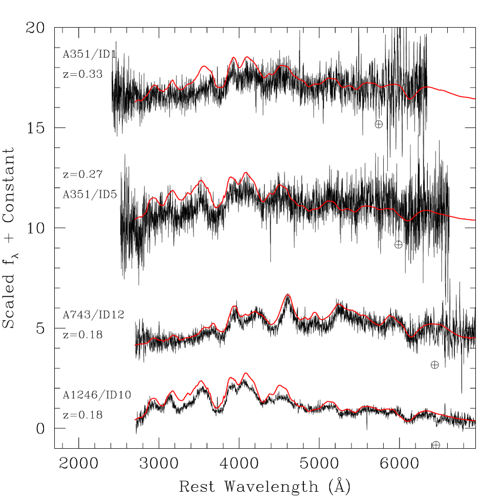
Figure 1.— Rest wavelength spectra of SNe Ia. Overplotted are SNe Ia template spectra from Peter Nugent (Nugent et al. 2002).

Figure 2.— Spectra of six low redshift ($z<0.3$) galaxies. For a discussion, see § 6.4.

Figure 3.— Spectra of five high redshift QSOs. The location of the A-band atmospheric absorption feature is indicated with a telluric symbol. No attempt was made to remove this feature.

Figure 4.— Spectra of five intermediate redshift QSOs. The location of the A-band atmospheric absorption feature is indicated with a telluric symbol. No attempt was made to remove this feature.

Figure 5.— Spectra of five variable stars. The location of the A-band atmospheric absorption feature is indicated with a telluric symbol. No attempt was made to remove this feature.

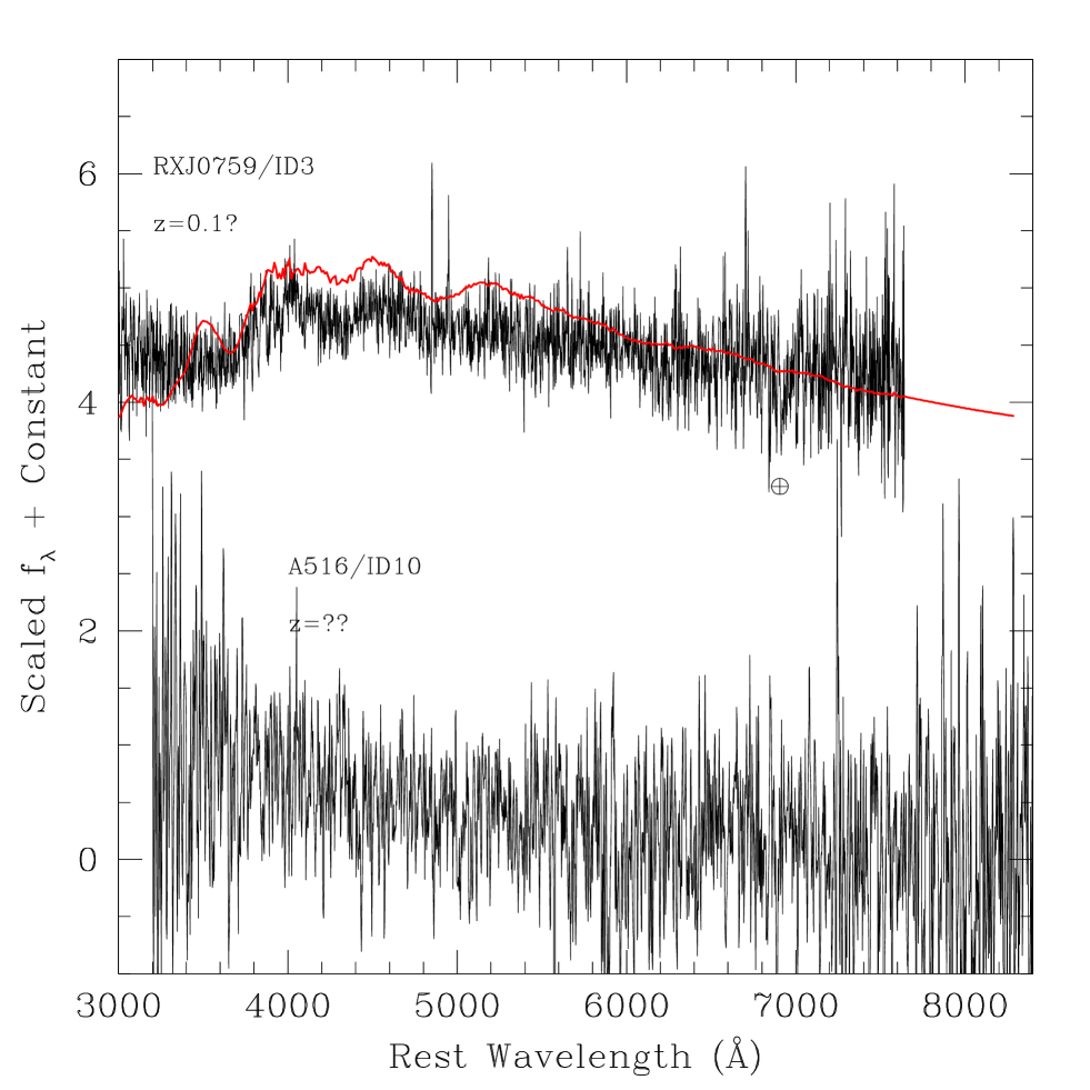
Figure 6.— Spectra of two unknown objects, although we suspect that the top spectrum may be a SNI b/c roughly eight days past explosion at a redshift of $z=0.1$, with some obvious galaxy contamination. We overplot a template SN spectrum with these characteristics using the template of Nugent et al. (2002). Even though Abell 516/ID10 was very faint at discovery, we devoted some spectroscopic resources to it since it was an apparent IC event. The location of the A-band atmospheric absorption feature is indicated with a telluric symbol. No attempt was made to remove this feature.

Radial profile of the variable sources as a function of clustercentric radius, scaled by $r_{200}$. All values have been renormalized to account for the different areas probed by the radial bins (including masked regions). All of the clusters have been probed out to $r_{200}$. The ’background’ transient rate is represented by the horizontal bar and was measured from chip 3.

Examples of template $g$ band SN Ia light curves at the redshift edges of our cluster sample ($0.1<z<0.2$).

Table 1List of Cluster Fields

Cluster	$z_{clus}$	$\alpha$	$\delta$	$L_{X}$	Epoch 1	Epoch 2	Epoch 3	Epoch 4
		(J2000.0)	(J2000.0)	[$10^{44}{\rm ergs\ s}^{-1}]$
A2703	0.114	00:05:30.6	+16:5:11.9	2.72	11/18/06	12/15/06
A136	0.157	01:04:14.4	+25:05:03.9	1.32	11/17/06	12/15/06
A351	0.105	02:25:42.3	-08:40:21.8	0.21	11/18/06	12/15/06
Z0256	0.194	02:59:32.6	+00:13:56.1	0.85	11/17/06	12/15/06
A516	0.141	04:50:24.9	-08:49:24.6	0.17	11/18/06	12/15/06
A565	0.105	07:06:54.0	+71:40:56.0	1.36	01/28/06	02/24/06	04/22/06
A572	0.104	07:14:18.7	+54:41:03.1	1.38	01/28/06	02/24/06	04/24/06
A580	0.118	07:25:57.2	+41:23:07.7	1.90	01/28/06	02/24/06	04/23/06
RXJ0759	0.104	07:59:41.1	+54:00:25.7	1.97	01/28/06	04/23/06	12/15/06
RXJ0804	0.187	08:04:21.4	+46:47:12.9	2.40	01/28/06	02/24/06	04/23/06	12/15/06
A667	0.145	08:28:06.4	+44:46:03.6	4.45	01/28/06	02/24/06	04/23/06
A750	0.163	09:09:12.7	+10:58:29.3	8.74	01/28/06	02/24/06	04/23/06
A853	0.165	09:42:15.0	+15:22:53.3	4.06	01/28/06	02/24/06	04/24/06
A961	0.124	10:16:23.2	+33:38:19.8	3.12	01/28/06	02/24/06	04/23/06
A1201	0.169	11:12:54.6	+13:26:09.8	6.05	01/28/06	04/23/06
A1413	0.143	11:55:18.2	+23:24:12.4	10.83	01/28/06	02/24/06	04/23/06
A1689	0.183	13:11:29.9	-01:20:33.3	20.95	01/28/06	02/24/06	04/23/06	06/19/06
A1361	0.117	11:43:39.7	+46:21:20.4	4.95	01/28/06	02/24/06	04/23/06
RXJ0741	0.158	07:41:26.7	+25:58:30.6	1.00	01/29/06	02/25/06	04/24/06
A620	0.135	08:05:43.2	+45:41:02.3	1.47	01/29/06	02/25/06	12/15/06
A665	0.182	08:30:57.4	+65:50:28.3	15.17	01/29/06	02/25/06
A743	0.133	09:06:44.9	+10:19:03.6	2.64	04/24/06	12/15/06
RXJ0958	0.147	09:58:12.5	+23:46:44.3	1.96	01/29/06	02/25/06	04/24/06
RXJ1000	0.153	10:00:31.0	+44:08:44.6	2.75	02/25/06	04/24/06
A868	0.153	09:45:26.5	-08:39:06.7	4.60	01/29/06	02/25/06
A901	0.170	09:55:57.4	-09:59:01.8	10.73	01/29/06	02/25/06
A1045	0.138	10:35:0.4	+30:41:40.3	3.53	01/29/06	02/25/06	04/24/06
A1068	0.138	10:40:44.8	+39:57:10.1	5.94	01/29/06	02/25/06	04/24/06	12/15/06
A990	0.144	10:23:39.9	+49:08:40.1	6.71	01/29/06	02/25/06	04/25/06
A1264	0.127	11:27:01.8	+17:07:47.7	2.07	01/29/06	02/25/06
A1246	0.190	11:23:58.8	+21:28:49.0	6.31	01/29/06	02/24/06	12/15/06
A1553	0.165	12:30:48.9	+10:32:48.4	7.19	01/29/06	02/24/06	04/23/06
A1204	0.171	11:13:20.5	+17:35:41.0	6.50	01/29/06	02/25/06	04/24/06
Z1432	0.189	07:51:25.0	+17:30:50.4	5.18	01/30/06	04/25/06
A646	0.129	08:22:09.3	+47:05:49.3	4.94	01/30/06	02/26/06	12/15/06
RXJ0821	0.110	08:21:02.0	+07:51:48.8	1.39	01/30/06	02/26/06	12/15/06
Z1883	0.194	08:42:56.0	+29:27:26.9	6.21	01/30/06	02/26/06
A655	0.127	08:25:28.8	+47:08:04.1	4.90	01/30/06	02/26/06
RXJ0819	0.119	08:19:25.7	+63:37:26.1	2.80	01/30/06	02/26/06
A795	0.136	09:24:05.4	14:10:24.2	5.70	01/30/06	02/26/06
A923	0.116	10:06:38.9	+25:54:44.5	2.05	01/30/06	02/26/06
A1033	0.126	10:31:44.3	+35:02:28.3	5.12	01/30/06	04/25/06	12/15/06
A1132	0.136	10:58:23.7	+56:47:42.7	6.76	01/30/06	04/25/06
A1111	0.165	10:50:46.7	-02:21:24.1	4.12	01/30/06	02/25/06
Z3179	0.143	10:25:58.1	+12:41:10.6	4.71	01/30/06	04/25/06
RXJ1156	0.142	11:56:55.8	+24:15:37.4	3.10	01/30/06	04/25/06
A1235	0.104	11:22:16.0	+19:35:49.3	1.70	01/30/06	02/25/06	04/25/06	12/15/06
A1366	0.116	11:44:36.9	+67:24:23.5	3.91	01/30/06	02/25/06	04/25/06
A1902	0.160	14:21:40.5	+37:17:32.6	4.55	04/23/06	06/19/06
A1677	0.183	13:05:50.8	+30:54:13.7	5.37	04/24/06	06/19/06
A1914	0.171	14:25:56.7	+37:48:59.0	17.30	04/24/06	06/19/06
A1930	0.131	14:32:38.0	+31:38:50.5	3.99	04/24/06	06/19/06
A2259	0.164	17:20:09.9	+27:40:08.9	5.95	04/25/06	06/19/06
A2218	0.176	16:35:49.6	+66:12:44.8	9.55	04/25/06	06/19/06
RXJ1750	0.171	17:50:17.0	+35:04:59.7	5.34	04/25/06	06/19/06

Table 2Summary of Intracluster SNe Candidates

Cluster	$\alpha$	$\delta$	$g$	$R_{BCG}$	$R_{BCG}/r_{200}$	$m_{lim,g}$	$M_{lim,g}$
	(J2000.0)	(J2000.0)	[mag]	[kpc]
A516	04:49:42.5	$-$08:51:42.2	23.83 $\pm$ 0.90	1595	2.0	25.1	$-$14.0
A1201	11:13:12.6	+13:12:10.3	22.52 $\pm$ 0.09	2537	1.4	25.3	$-$14.3
A1413	11:56:9.63	+23:32:29.4	22.12 $\pm$ 0.05	2172	1.0	26.1	$-$13.1
A2259	17:23:33.4	+27:49:31.6	22.54 $\pm$ 0.08	7764	4.2	25.3	$-$14.2

Table 3List of Identified Variables – Cluster Centered Chip 1

Cluster	Epoch	$\alpha$	$\delta$	$g$	Dist from BCG	Notes
		(J2000.0)	J2000.0	mag	kpc
A136	2006-12-16 02:43:01	1:3:19.9	25:4:28.4	24.51 $\pm$ 0.60	2012	z=0.172 galaxy; BCS
A136	2006-12-16 02:43:01	1:4:2.14	25:7:22.8	22.91 $\pm$ 0.12	589
A136	2006-12-16 02:43:01	1:3:55.5	24:50:20.5	21.75 $\pm$ 0.06	2498	z=0.246 galaxy; BCS
A351	2006-12-16 03:57:01	2:26:21.3	-8:54:19.8	22.71 $\pm$ 0.17	1961	SN 2006ub; SNIa; BCS
A351	2006-12-16 03:57:01	2:25:56.9	-8:45:38.3	21.71 $\pm$ 0.07	740	SN 2006ua; SNIa; BCS
Z0256	2006-12-16 05:11:56	2:59:35.2	0:18:38.6	22.87 $\pm$ 0.14	919
Z0256	2006-12-16 05:11:56	2:59:7.80	0:22:33.9	22.81 $\pm$ 0.14	2054	z=0.199 CG; BCS
Z0256	2006-12-16 05:11:56	3:0:18.8	0:19:11.6	23.59 $\pm$ 0.31	2455
Z0256	2006-12-16 05:11:56	3:0:15.3	0:13:28.4	22.57 $\pm$ 0.14	2069
A516	2006-12-16 04:34:40	4:49:42.5	-8:51:42.2	23.83 $\pm$ 0.90	1595	?; BCS; IC Cand
A516	2006-12-16 04:34:40	4:50:52.5	-8:45:3.96	22.09 $\pm$ 0.07	1206	Stellar spec; BCS
A516	2006-12-16 04:34:40	4:50:29.1	-8:50:2.11	22.93 $\pm$ 0.19	183	Stellar spec; BCS
A743	2006-04-25 05:12:57	9:7:25.7	10:24:30.9	21.54 $\pm$ 0.06	1620
A743	2006-12-16 08:53:47	9:6:55.2	10:14:13.6	22.00 $\pm$ 0.09	775	z=0.267 Galaxy; BCS
A743	2006-12-16 08:53:47	9:6:32.4	10:9:29.1	21.32 $\pm$ 0.05	1425	SN 2006ud; SNIa; BCS
A743	2006-12-16 08:53:47	9:7:12.5	10:23:34.9	22.29 $\pm$ 0.12	1158
A565	2006-01-28 02:42:49	7:7:26.8	71:44:42.2	22.14 $\pm$ 0.09	528
A565	2006-02-24 02:13:37	7:9:33.9	71:34:49.1	21.52 $\pm$ 0.05	1622
A565	2006-04-23 03:04:32	7:10:10.5	71:50:20.4	21.56 $\pm$ 0.07	2077
A565	2006-04-23 03:04:32	7:7:49.4	71:52:31.6	21.93 $\pm$ 0.09	1429
A572	2006-02-24 02:48:27	7:15:26.0	54:37:29.0	21.80 $\pm$ 0.04	1188
A572	2006-02-24 02:48:27	7:14:11.5	54:26:52.5	23.12 $\pm$ 0.15	1628
A572	2006-02-24 02:48:27	7:13:8.08	54:26:39.5	22.93 $\pm$ 0.14	2025
A572	2006-02-24 02:48:27	7:12:56.3	54:28:31.2	21.03 $\pm$ 0.03	1984
A572	2006-02-24 02:48:27	7:12:38.0	54:41:0.311	20.90 $\pm$ 0.02	1666
A572	2006-04-25 03:15:23	7:13:46.5	54:38:22.6	22.15 $\pm$ 0.06	615
A572	2006-04-25 03:15:23	7:13:25.1	54:42:15.0	23.23 $\pm$ 0.18	897
A580	2006-02-24 03:49:52	7:26:15.1	41:37:34.2	21.71 $\pm$ 0.04	1897	RD
A580	2006-04-24 03:05:59	7:25:5.34	41:32:48.4	22.15 $\pm$ 0.07	1753
A580	2006-04-24 03:05:59	7:26:22.4	41:24:43.2	21.87 $\pm$ 0.06	640	z=1.803 QSO; SDSS
A580	2006-04-24 03:05:59	7:26:20.5	41:14:48.2	20.40 $\pm$ 0.02	1204
A580	2006-04-24 03:05:59	7:26:15.1	41:37:34.2	20.76 $\pm$ 0.02	1897	RD
A580	2006-04-24 03:05:59	7:26:12.5	41:22:34.1	22.20 $\pm$ 0.08	375	CG; SDSS
RXJ0759	2006-01-28 05:07:38	8:0:37.4	53:47:50.4	22.01 $\pm$ 0.06	1728
RXJ0759	2006-01-28 05:07:38	7:59:17.3	54:2:32.0	22.19 $\pm$ 0.07	466
RXJ0759	2006-01-28 05:07:38	7:58:34.4	54:10:30.8	21.93 $\pm$ 0.06	1607
RXJ0759	2006-04-24 03:52:36	7:59:40.3	53:55:49.2	22.64 $\pm$ 0.10	528
RXJ0759	2006-04-24 03:52:36	7:58:32.1	54:6:42.1	22.71 $\pm$ 0.10	1362	RD
RXJ0759	2006-12-16 09:36:16	8:0:46.0	53:47:15.5	22.59 $\pm$ 0.07	1866
RXJ0759	2006-12-16 09:36:16	7:59:52.3	53:47:44.5	21.27 $\pm$ 0.02	1466
RXJ0759	2006-12-16 09:36:16	7:59:13.0	54:4:42.2	22.20 $\pm$ 0.04	680	z=2.93 QSO; BCS
RXJ0759	2006-12-16 09:36:16	7:58:45.9	54:1:17.4	22.09 $\pm$ 0.04	934	SN 2006uc; SNIa; BCS
RXJ0759	2006-12-16 09:36:16	7:58:32.1	54:6:42.9	22.71 $\pm$ 0.06	1363	RD
RXJ0804	2006-01-28 06:15:30	8:5:10.2	46:43:32.8	21.98 $\pm$ 0.04	1716
RXJ0804	2006-02-24 05:20:32	8:5:6.84	46:35:19.0	22.58 $\pm$ 0.07	2672
RXJ0804	2006-02-24 05:20:32	8:4:28.0	46:48:15.8	22.40 $\pm$ 0.06	292
RXJ0804	2006-02-24 05:20:32	8:4:24.6	46:56:55.1	22.08 $\pm$ 0.04	1825
RXJ0804	2006-02-24 05:20:32	8:4:8.89	46:39:10.9	19.13 $\pm$ 0.00	1561
RXJ0804	2006-04-24 04:33:50	8:2:51.8	46:48:42.9	23.72 $\pm$ 0.32	2890
RXJ0804	2006-12-16 07:07:14	8:5:18.5	46:35:40.3	21.60 $\pm$ 0.03	2845	z=1.775 (phot) QSO/1
RXJ0804	2006-12-16 07:07:14	8:3:24.0	46:55:18.9	21.95 $\pm$ 0.06	2386
RXJ0804	2006-12-16 07:07:14	8:3:12.9	46:58:12.1	21.90 $\pm$ 0.05	3010	z=1.775 (phot) QSO/1
RXJ0804	2006-12-16 07:07:14	8:4:50.2	47:1:45.2	21.70 $\pm$ 0.05	2881
RXJ0804	2006-12-16 07:07:14	8:4:21.4	46:57:15.4	22.83 $\pm$ 0.11	1885
RXJ0804	2006-12-16 07:07:14	8:3:57.0	46:40:37.7	22.32 $\pm$ 0.07	1465
A667	2006-01-28 06:52:55	8:28:49.1	44:44:38.0	20.47 $\pm$ 0.01	1177	RD
A667	2006-01-28 06:52:55	8:28:31.9	44:34:3.13	22.24 $\pm$ 0.06	1958
A667	2006-01-28 06:52:55	8:28:15.9	44:47:24.2	22.29 $\pm$ 0.07	329
A667	2006-02-24 05:57:42	8:27:9.95	44:29:25.1	24.18 $\pm$ 0.47	2966
A667	2006-04-24 05:11:06	8:28:49.1	44:44:38.0	20.73 $\pm$ 0.02	1177	RD
A667	2006-04-24 05:11:06	8:26:41.5	44:55:37.4	23.25 $\pm$ 0.22	2716
A750	2006-04-24 05:49:13	9:9:47.8	11:6:36.6	22.34 $\pm$ 0.09	1991
A853	2006-01-28 08:36:18	9:43:12.5	15:35:9.70	22.00 $\pm$ 0.13	3140
A853	2006-01-28 08:36:18	9:42:53.6	15:26:4.16	22.00 $\pm$ 0.12	1672
A961	2006-02-24 07:52:05	10:17:29.6	33:45:15.6	22.83 $\pm$ 0.12	2063
A1201	2006-01-28 10:18:32	11:13:36.0	13:38:31.0	22.57 $\pm$ 0.10	2759
A1201	2006-01-28 10:18:32	11:12:17.8	13:21:6.03	21.55 $\pm$ 0.04	1779	z=0.231 QSO; SDSS
A1201	2006-04-24 07:09:10	11:13:29.0	13:34:42.0	22.87 $\pm$ 0.12	2070
A1201	2006-04-24 07:09:10	11:13:12.6	13:12:10.3	22.52 $\pm$ 0.09	2537	IC Cand
A1201	2006-04-24 07:09:10	11:12:47.5	13:14:4.21	21.95 $\pm$ 0.05	2114	QSO z=1.524; SDSS
A1413	2006-01-28 11:09:51	11:55:50.3	23:23:58.5	22.49 $\pm$ 0.08	1112
A1413	2006-01-28 11:09:51	11:55:4.32	23:31:18.7	22.19 $\pm$ 0.07	1173
A1413	2006-02-24 09:06:07	11:56:9.63	23:32:29.4	22.12 $\pm$ 0.05	2171	IC Cand
A1413	2006-02-24 09:06:07	11:56:5.11	23:11:16.5	23.64 $\pm$ 0.24	2537
A1413	2006-02-24 09:06:07	11:55:46.6	23:24:47.8	21.59 $\pm$ 0.04	989
A1413	2006-04-24 07:59:00	11:55:55.2	23:15:44.3	21.56 $\pm$ 0.03	1808
A1413	2006-04-24 07:59:00	11:55:44.4	23:37:29.5	22.29 $\pm$ 0.07	2198
A1413	2006-04-24 07:59:00	11:55:42.0	23:28:55.6	22.03 $\pm$ 0.06	1088
A1689	2006-01-28 11:51:19	13:10:50.2	-1:24:20.7	18.85 $\pm$ 0.00	1958	RD QUEST 088049/3
A1689	2006-01-28 11:51:19	13:12:6.64	-1:31:30.2	21.35 $\pm$ 0.03	2637	RD z=0.845 QSO/4
A1689	2006-01-28 11:51:19	13:11:55.8	-1:25:56.6	22.30 $\pm$ 0.07	1555	RD z=0.962 QSO/4
A1689	2006-01-28 11:51:19	13:11:52.6	-1:23:4.82	21.62 $\pm$ 0.04	1150	CG/5
A1689	2006-01-28 11:51:19	13:11:35.6	-1:9:26.1	22.09 $\pm$ 0.06	2069
A1689	2006-01-28 11:51:19	13:11:29.6	-1:16:2.60	22.43 $\pm$ 0.08	833	z=1.648 QSO/4
A1689	2006-02-24 09:46:20	13:12:6.64	-1:31:30.2	21.82 $\pm$ 0.05	2637	RD z=0.845 QSO/4
A1689	2006-02-24 09:46:20	13:12:5.77	-1:30:8.38	22.75 $\pm$ 0.12	2422
A1689	2006-02-24 09:46:20	13:11:59.8	-1:28:5.43	22.36 $\pm$ 0.16	1958
A1689	2006-02-24 09:46:20	13:11:55.8	-1:25:56.1	22.64 $\pm$ 0.11	1554	RD z=0.962 QSO/4
A1689	2006-04-24 08:39:34	13:11:19.3	-1:20:30.2	22.11 $\pm$ 0.07	485	z=2.584 QSO/6
A1689	2006-04-24 08:39:34	13:11:18.3	-1:14:29.4	21.44 $\pm$ 0.03	1239	2QZ J131118.2-011430/4
A1689	2006-04-24 08:39:34	13:10:55.5	-1:27:25.1	21.63 $\pm$ 0.04	2029	z=1.003 QSO/6
A1689	2006-06-19 04:03:19	13:12:28.0	-1:21:37.9	21.50 $\pm$ 0.04	2689
A1689	2006-06-19 04:03:19	13:10:57.6	-1:20:42.4	22.16 $\pm$ 0.08	1488
A1689	2006-06-19 04:03:19	13:10:50.2	-1:24:20.7	18.64 $\pm$ 0.00	1958	RD QUEST 088049/3
A1361	2006-01-28 12:29:23	11:44:20.2	46:28:29.6	18.56 $\pm$ 0.00	1269	RD
A1361	2006-01-28 12:29:23	11:43:44.1	46:23:0.144	21.70 $\pm$ 0.03	232
A1361	2006-04-24 09:20:33	11:44:21.4	46:23:4.06	22.77 $\pm$ 0.10	940
A1361	2006-04-24 09:20:33	11:44:20.2	46:28:30.0	18.58 $\pm$ 0.00	1270	RD
A1361	2006-04-24 09:20:33	11:42:23.4	46:26:11.0	22.24 $\pm$ 0.08	1778
RXJ0741	2006-01-29 02:11:06	7:42:18.1	25:53:45.7	21.85 $\pm$ 0.07	2048	RD
RXJ0741	2006-01-29 02:11:06	7:41:26.6	26:7:36.5	21.20 $\pm$ 0.05	1490
RXJ0741	2006-02-25 02:26:30	7:42:18.1	25:53:45.7	21.75 $\pm$ 0.06	2048	RD
RXJ0741	2006-02-25 02:26:30	7:40:34.2	26:3:31.5	22.29 $\pm$ 0.10	2097
RXJ0741	2006-02-25 02:26:30	7:41:18.4	25:44:14.1	21.97 $\pm$ 0.09	2357
RXJ0741	2006-04-25 03:53:15	7:40:52.7	25:51:51.3	22.97 $\pm$ 0.17	1658
A620	2006-01-29 02:55:40	8:6:14.7	45:35:45.0	21.95 $\pm$ 0.05	1098	RD Stellar spec; BCS
A620	2006-02-25 03:05:49	8:4:35.6	45:31:0.928	22.23 $\pm$ 0.08	2227	CG; SDSS
A620	2006-02-25 03:05:49	8:5:6.89	45:32:37.7	21.20 $\pm$ 0.03	1513	RD Stellar spec; BCS
A620	2006-12-16 05:52:00	8:5:6.89	45:32:37.7	21.70 $\pm$ 0.06	1513	RD Stellar spec; BCS
A620	2006-12-16 05:52:00	8:6:14.7	45:35:45.5	21.19 $\pm$ 0.04	1097	RD Stellar spec; BCS
A665	2006-01-29 04:31:29	8:30:1.46	65:45:2.30	21.92 $\pm$ 0.05	1453	CG/7
RXJ0958	2006-01-29 05:54:09	9:57:15.9	23:41:16.2	23.36 $\pm$ 0.37	2166	RD
RXJ0958	2006-02-25 05:03:22	9:57:15.9	23:41:16.7	22.29 $\pm$ 0.13	2167	RD
RXJ1000	2006-02-25 05:39:58	10:1:31.3	44:1:45.4	22.23 $\pm$ 0.06	2057
RXJ1000	2006-04-25 07:19:59	9:59:47.7	44:15:18.8	22.89 $\pm$ 0.09	1618
RXJ1000	2006-04-25 07:19:59	9:59:24.1	43:54:57.9	22.70 $\pm$ 0.11	2917
A868	2006-02-25 06:16:49	9:46:19.4	-8:49:27.9	22.08 $\pm$ 0.07	2661
A901	2006-01-29 07:46:57	9:57:0.0908	-9:53:9.53	20.76 $\pm$ 0.02	2872
A901	2006-01-29 07:46:57	9:56:33.7	-10:8:24.7	21.66 $\pm$ 0.04	2253
A901	2006-02-25 06:53:39	9:55:34.2	-9:51:15.2	21.31 $\pm$ 0.04	1677
A1045	2006-04-25 07:58:26	10:34:41.5	30:47:3.26	21.92 $\pm$ 0.06	985
A1045	2006-04-25 07:58:26	10:34:39.0	30:53:36.8	21.22 $\pm$ 0.03	1871
A1068	2006-02-25 08:14:53	10:41:46.4	39:47:24.7	20.65 $\pm$ 0.06	2244
A1068	2006-02-25 08:14:53	10:40:34.4	39:45:9.89	21.61 $\pm$ 0.16	1780
A1068	2006-04-25 08:35:17	10:39:37.3	39:56:40.8	22.06 $\pm$ 0.14	1894
A1068	2006-12-16 11:35:39	10:39:27.2	40:8:58.5	23.80 $\pm$ 0.26	2772
A1068	2006-12-16 11:35:39	10:41:8.21	39:49:24.3	22.27 $\pm$ 0.05	1312
A1068	2006-12-16 11:35:39	10:39:42.1	39:47:22.3	22.81 $\pm$ 0.10	2270
A990	2006-01-29 09:51:56	10:22:15.2	49:2:7.73	23.03 $\pm$ 0.25	2326
A990	2006-02-25 08:52:41	10:23:44.4	48:57:16.6	22.27 $\pm$ 0.07	1731
A990	2006-04-26 05:39:01	10:23:45.3	49:16:47.7	23.57 $\pm$ 0.25	1239
A990	2006-04-26 05:39:01	10:23:34.2	49:11:15.5	21.93 $\pm$ 0.04	417
A990	2006-04-26 05:39:01	10:22:27.3	49:22:52.9	22.64 $\pm$ 0.16	2802
A1264	2006-01-29 10:29:19	11:27:24.3	17:11:23.7	22.08 $\pm$ 0.11	884
A1264	2006-01-29 10:29:19	11:26:41.2	17:3:10.9	21.97 $\pm$ 0.09	919
A1264	2006-02-25 09:33:14	11:26:38.3	17:9:53.2	22.10 $\pm$ 0.14	814
A1264	2006-02-25 09:33:14	11:26:34.6	17:3:51.1	22.11 $\pm$ 0.12	1035
A1246	2006-12-16 12:11:23	11:24:48.9	21:36:5.22	21.45 $\pm$ 0.02	2614	z=0.92 QSO; BCS
A1246	2006-12-16 12:11:23	11:24:41.5	21:12:9.94	24.46 $\pm$ 0.46	3689
A1246	2006-12-16 12:11:23	11:24:2.51	21:36:58.1	22.54 $\pm$ 0.06	1559	Stellar spec; BCS
A1246	2006-12-16 12:11:23	11:23:49.5	21:28:40.3	20.63 $\pm$ 0.01	411	SN 2006ue; Cluster SNIa; BCS
A1553	2006-01-29 11:52:37	12:31:16.9	10:48:35.9	22.62 $\pm$ 0.17	2924
A1553	2006-01-29 11:52:37	12:30:50.5	10:39:0.640	22.58 $\pm$ 0.13	1055	z=0.213 QSO; SDSS
A1553	2006-02-24 11:45:49	12:30:10.6	10:23:11.6	22.69 $\pm$ 0.20	2283
A1553	2006-04-24 10:03:28	12:30:45.8	10:32:50.4	22.34 $\pm$ 0.11	126
A1553	2006-04-24 10:03:28	12:31:22.2	10:44:12.8	21.75 $\pm$ 0.06	2383	z=0.092 Galaxy; SDSS
A1204	2006-01-29 12:31:42	11:12:55.8	17:37:36.7	22.14 $\pm$ 0.08	1078
A1204	2006-02-25 12:13:56	11:14:16.6	17:40:57.0	22.26 $\pm$ 0.09	2513
A1204	2006-04-25 09:11:22	11:13:59.2	17:39:2.83	22.06 $\pm$ 0.08	1718
A1204	2006-04-25 09:11:22	11:13:53.7	17:30:14.0	21.93 $\pm$ 0.07	1681
Z1432	2006-01-30 02:02:53	7:52:22.8	17:16:36.9	21.43 $\pm$ 0.10	3754
Z1432	2006-02-26 02:29:16	7:51:54.2	17:21:43.8	21.83 $\pm$ 0.06	2173
Z1432	2006-02-26 02:29:16	7:51:20.7	17:38:58.1	22.52 $\pm$ 0.38	1551
A646	2006-12-16 10:22:04	8:22:7.01	46:56:0.475	21.03 $\pm$ 0.07	1356	z=2.325 (phot) QSO/1
A646	2006-12-16 10:22:04	8:21:5.55	47:16:33.4	21.40 $\pm$ 0.10	2104	z=2.22 QSO; BCS
A646	2006-12-16 10:22:04	8:22:32.4	47:14:45.3	21.25 $\pm$ 0.09	1348
RXJ0821	2006-01-30 03:29:06	8:21:52.2	7:39:4.20	22.57 $\pm$ 0.13	2145
RXJ0821	2006-01-30 03:29:06	8:20:43.0	7:41:24.6	21.22 $\pm$ 0.04	1374	RD
RXJ0821	2006-01-30 03:29:06	8:20:42.6	8:3:56.1	22.32 $\pm$ 0.10	1569
RXJ0821	2006-01-30 03:29:06	8:20:29.5	7:54:27.1	22.21 $\pm$ 0.09	1017
RXJ0821	2006-01-30 03:29:06	8:20:28.5	7:41:6.98	22.95 $\pm$ 0.19	1629	RD
RXJ0821	2006-01-30 03:29:06	8:21:21.2	7:42:1.31	22.13 $\pm$ 0.08	1311	RD
RXJ0821	2006-01-30 03:29:06	8:21:14.9	7:40:31.0	22.62 $\pm$ 0.13	1413
RXJ0821	2006-01-30 03:29:06	8:20:52.3	7:55:35.4	22.06 $\pm$ 0.07	537	RD z=1.13 QSO; SDSS
RXJ0821	2006-01-30 03:29:06	8:20:45.6	8:3:25.8	21.77 $\pm$ 0.07	1480	z=2.91 QSO; SDSS
RXJ0821	2006-02-26 04:02:42	8:21:21.2	7:42:1.31	22.31 $\pm$ 0.10	1311	RD
RXJ0821	2006-02-26 04:02:42	8:21:18.0	7:53:59.2	22.60 $\pm$ 0.13	544	X-ray pt src/2
RXJ0821	2006-02-26 04:02:42	8:20:52.4	7:55:34.9	22.24 $\pm$ 0.09	536	RD z=1.13 QSO; SDSS
RXJ0821	2006-02-26 04:02:42	8:20:43.0	7:41:24.6	21.40 $\pm$ 0.04	1374	RD
RXJ0821	2006-02-26 04:02:42	8:20:28.5	7:41:6.08	22.59 $\pm$ 0.14	1630	RD
RXJ0821	2006-02-26 04:02:42	8:21:30.6	7:50:56.8	21.96 $\pm$ 0.08	860
RXJ0821	2006-02-26 04:02:42	8:21:21.6	7:46:25.9	22.99 $\pm$ 0.21	874
RXJ0821	2006-12-16 08:11:33	8:20:34.2	7:39:37.6	21.73 $\pm$ 0.07	1684	Galaxy z=0.22; BCS
RXJ0821	2006-12-16 08:11:33	8:20:22.1	7:38:12.1	22.41 $\pm$ 0.15	2023
RXJ0821	2006-12-16 08:11:33	8:20:19.2	7:53:24.7	21.84 $\pm$ 0.08	1288
RXJ0821	2006-12-16 08:11:33	8:21:23.0	7:39:41.3	22.20 $\pm$ 0.11	1588	z=0.90 QSO; BCS
RXJ0821	2006-12-16 08:11:33	8:21:16.3	8:3:38.1	22.48 $\pm$ 0.14	1485
RXJ0821	2006-12-16 08:11:33	8:20:52.7	7:52:38.8	21.96 $\pm$ 0.08	294	z=0.795 QSO; BCS
RXJ0821	2006-12-16 08:11:33	8:20:44.5	7:50:7.56	22.43 $\pm$ 0.13	558	z=2.17 QSO; BCS
Z1883	2006-01-30 04:05:53	8:43:19.7	29:23:48.4	22.03 $\pm$ 0.06	1221
A655	2006-01-30 04:42:47	8:25:49.6	47:10:28.4	17.45 $\pm$ 0.01	583	CG AGN; SDSS/8
RXJ0819	2006-01-30 05:19:40	8:17:52.7	63:42:0.576	22.99 $\pm$ 0.36	1451
RXJ0819	2006-01-30 05:19:40	8:17:48.2	63:33:58.4	23.42 $\pm$ 0.56	1467
RXJ0819	2006-02-26 06:25:49	8:19:39.7	63:45:46.4	20.36 $\pm$ 0.02	1093
RXJ0819	2006-02-26 06:25:49	8:18:11.7	63:45:21.8	22.36 $\pm$ 0.13	1467
A795	2006-01-30 05:56:39	9:24:58.8	13:56:55.7	22.01 $\pm$ 0.23	2703
A795	2006-01-30 05:56:39	9:24:40.2	14:20:6.92	20.88 $\pm$ 0.09	1858
A795	2006-01-30 05:56:39	9:24:4.61	13:56:16.7	18.99 $\pm$ 0.01	2041
A795	2006-01-30 05:56:39	9:23:49.6	14:6:25.6	22.08 $\pm$ 0.24	797
A1033	2006-01-30 07:14:07	10:31:58.6	35:1:17.9	21.72 $\pm$ 0.04	427
A1033	2006-04-26 06:14:44	10:32:35.3	34:57:8.35	21.78 $\pm$ 0.04	1589	RD
A1033	2006-04-26 06:14:44	10:32:28.9	35:2:7.13	20.33 $\pm$ 0.01	1238	z=0.128 QSO; CG; SDSS
A1033	2006-12-16 10:58:20	10:32:40.5	34:58:35.8	22.64 $\pm$ 0.10	1646	z=1.56 BAL QSO; BCS
A1033	2006-12-16 10:58:20	10:32:35.2	34:57:8.41	22.62 $\pm$ 0.09	1587	RD
A1033	2006-12-16 10:58:20	10:31:31.0	35:16:23.7	22.77 $\pm$ 0.10	1920
A1033	2006-12-16 10:58:20	10:30:31.9	34:56:47.9	23.16 $\pm$ 0.19	2149	SNIb/c?; BCS
A1132	2006-01-30 07:50:49	10:59:6.18	56:59:46.8	22.30 $\pm$ 0.08	1934
A1132	2006-01-30 07:50:49	10:58:48.6	56:48:0.285	22.03 $\pm$ 0.06	496
A1132	2006-01-30 07:50:49	10:57:35.2	56:53:23.7	22.49 $\pm$ 0.11	1260
Z3179	2006-01-30 09:50:19	10:25:20.4	12:34:45.2	22.21 $\pm$ 0.08	1689	z=1.489 QSO; SDSS
RXJ1156	2006-01-30 10:29:24	11:57:30.6	24:27:43.2	21.26 $\pm$ 0.03	2168
RXJ1156	2006-04-26 08:16:34	11:57:37.9	24:14:43.4	22.42 $\pm$ 0.08	1447
RXJ1156	2006-04-26 08:16:34	11:56:27.6	24:12:26.9	21.68 $\pm$ 0.04	1072
RXJ1156	2006-04-26 08:16:34	11:56:25.0	24:8:37.4	21.99 $\pm$ 0.05	1484
RXJ1156	2006-04-26 08:16:34	11:56:20.4	24:18:52.6	22.63 $\pm$ 0.09	1301
RXJ1156	2006-04-26 08:16:34	11:56:9.60	24:9:43.5	22.31 $\pm$ 0.08	1809
RXJ1156	2006-04-26 08:16:34	11:56:7.56	24:8:39.3	23.11 $\pm$ 0.16	1951
A1235	2006-01-30 11:09:02	11:22:51.3	19:35:51.5	22.43 $\pm$ 0.10	664
A1235	2006-01-30 11:09:02	11:22:26.1	19:23:0.141	20.69 $\pm$ 0.03	1993
A1235	2006-12-16 12:47:19	11:22:19.7	19:47:5.33	21.91 $\pm$ 0.11	1991
A1235	2006-12-16 12:47:19	11:22:12.7	19:35:57.9	20.73 $\pm$ 0.04	1706
A1235	2006-12-16 12:47:19	11:23:18.8	19:44:17.4	22.00 $\pm$ 0.12	973
A1235	2006-12-16 12:47:19	11:22:51.3	19:28:34.6	20.97 $\pm$ 0.05	1065
A1235	2006-12-16 12:47:19	11:22:44.9	19:48:37.7	21.47 $\pm$ 0.07	1689
A1366	2006-04-26 09:30:39	11:46:48.9	67:37:6.08	21.81 $\pm$ 0.05	2253	z=1.539 QSO; SDSS
A1366	2006-04-26 09:30:39	11:43:10.3	67:32:5.47	22.73 $\pm$ 0.11	1424
A1902	2006-04-24 10:42:43	14:21:51.9	37:5:57.8	22.40 $\pm$ 0.08	1953
A1902	2006-04-24 10:42:43	14:21:29.6	37:11:20.7	21.69 $\pm$ 0.04	1085
A1902	2006-04-24 10:42:43	14:20:59.2	37:10:57.7	22.46 $\pm$ 0.09	1741
A1902	2006-06-19 05:40:24	14:20:55.3	37:9:23.6	20.29 $\pm$ 0.01	2009
A1677	2006-04-25 09:50:29	13:5:58.3	30:56:29.6	21.10 $\pm$ 0.03	513
A1677	2006-06-19 04:59:20	13:6:6.00	30:47:28.2	22.70 $\pm$ 0.13	1385
A1914	2006-04-25 10:31:46	14:26:20.3	37:45:0.308	22.11 $\pm$ 0.05	1074
A1914	2006-06-19 06:24:29	14:25:28.4	37:45:39.9	22.31 $\pm$ 0.06	1133
A1930	2006-06-19 07:06:52	14:32:16.4	31:40:39.0	21.92 $\pm$ 0.05	690	z=0.129 QSO; CG; SDSS
A1930	2006-06-19 07:06:52	14:31:44.4	31:39:46.9	21.89 $\pm$ 0.04	1601
A2259	2006-04-26 10:10:35	17:20:56.0	27:38:12.5	18.53 $\pm$ 0.00	1757
A2259	2006-04-26 10:10:35	17:19:24.2	27:51:53.8	20.85 $\pm$ 0.02	2614
A2259	2006-06-19 08:31:34	17:19:27.1	27:32:45.7	21.52 $\pm$ 0.05	2028	z=1.447 QSO; SDSS
A2218	2006-06-19 07:49:38	16:34:2.04	66:15:47.7	21.96 $\pm$ 0.05	2011
RXJ1750	2006-04-26 11:26:39	17:49:36.4	35:9:55.6	18.85 $\pm$ 0.01	1685
RXJ1750	2006-04-26 11:26:39	17:50:57.1	35:14:47.0	19.85 $\pm$ 0.01	2231
RXJ1750	2006-06-19 09:09:59	17:50:57.2	35:12:10.3	22.76 $\pm$ 0.22	1906
RXJ1750	2006-06-19 09:09:59	17:49:23.7	35:7:15.8	21.93 $\pm$ 0.10	1942

Note. — The following abbreviations were used under the ’Notes’ column. BCS – Indicates that this transient was followed up spectroscopically by the Blue Channel Spectrograph on the MMT – see § 6. CG – Indicates that the transient is associated with a cluster galaxy. IC Cand – Intracluster SN candidate. RD – This transient was detected as a variable in more than one epoch

References. — (1) Richards et al. (2004); (2) Gandhi et al. (2004); (3) Rengstorf et al. (2004); (4) Croom et al. (2004); (5) Balogh et al. (2002); (6) Hewett et al. (1995); (7) Oegerle et al. (1991); (8) Vanden Berk et al. (2006)

Table 4List of Identified Variables – Background Chip 3

Cluster	Epoch	$\alpha$	$\delta$	g	Dist from BCG	Notes
		(J2000.0)	J2000.0	mag	kpc
RXJ1750	2006-04-26 11:26:39	17:53:2.73	35:5:57.7	20.95 $\pm$ 0.04	5925
RXJ1750	2006-04-26 11:26:39	17:52:46.3	35:7:9.76	21.72 $\pm$ 0.08	5349
A2218	2006-04-26 10:46:38	16:40:49.7	66:22:48.2	21.35 $\pm$ 0.03	5670
A2218	2006-04-26 10:46:38	16:40:42.8	66:11:10.9	22.32 $\pm$ 0.07	5302
A2259	2006-04-26 10:10:35	17:23:33.4	27:49:31.6	22.54 $\pm$ 0.08	7764	IC Cand
A2259	2006-04-26 10:10:35	17:22:7.20	27:26:29.7	21.87 $\pm$ 0.10	4963
A1677	2006-06-19 04:59:20	13:9:27.7	30:44:19.4	20.54 $\pm$ 0.02	8794
A1677	2006-06-19 04:59:20	13:9:3.27	31:6:26.6	22.18 $\pm$ 0.07	7930
A1689	2006-01-28 11:51:19	13:14:46.1	-1:8:52.2	21.92 $\pm$ 0.06	9305
A1689	2006-01-28 11:51:19	13:13:46.3	-1:13:19.2	22.07 $\pm$ 0.06	6431
A1689	2006-02-24 09:46:20	13:13:34.8	-1:18:3.00	22.17 $\pm$ 0.07	5781	z=1.675 (phot) QSO/1
A1689	2006-06-19 04:03:19	13:14:30.8	-1:29:45.9	20.82 $\pm$ 0.03	8514
A1689	2006-06-19 04:03:19	13:14:17.9	-1:35:12.1	22.13 $\pm$ 0.10	8208
A1689	2006-06-19 04:03:19	13:13:48.7	-1:25:39.3	22.12 $\pm$ 0.09	6472
A1902	2006-04-24 10:42:43	14:24:37.2	37:20:33.4	22.76 $\pm$ 0.16	5836
A1902	2006-04-24 10:42:43	14:26:2.16	37:3:4.55	21.92 $\pm$ 0.07	8965
A1914	2006-04-25 10:31:46	14:29:27.7	37:45:21.0	21.98 $\pm$ 0.05	7316	z=1.69 QSO; SDSS
A1914	2006-04-25 10:31:46	14:28:22.1	37:58:14.5	22.96 $\pm$ 0.10	5264
A1914	2006-06-19 06:24:29	14:30:9.63	38:0:41.9	22.19 $\pm$ 0.05	8942
A1930	2006-06-19 07:06:52	14:35:9.50	31:31:48.3	21.86 $\pm$ 0.04	4624	z=0.50 QSO; SDSS
A1930	2006-06-19 07:06:52	14:35:0.177	31:41:35.7	22.97 $\pm$ 0.17	4250
A1930	2006-06-19 07:06:52	14:34:55.9	31:39:24.5	21.93 $\pm$ 0.05	4108
A1553	2006-04-24 10:03:28	12:34:12.5	10:26:23.9	22.71 $\pm$ 0.16	8565
RXJ0958	2006-01-29 05:54:09	10:1:32.4	23:40:0.701	22.28 $\pm$ 0.10	7137
RXJ0958	2006-01-29 05:54:09	10:1:25.3	23:56:20.2	21.05 $\pm$ 0.03	6955
RXJ0958	2006-01-29 05:54:09	10:0:49.4	23:54:33.7	21.82 $\pm$ 0.06	5664	RD
RXJ0958	2006-01-29 05:54:09	10:0:7.77	23:44:56.0	22.60 $\pm$ 0.12	4078
RXJ0958	2006-02-25 05:03:22	10:0:49.4	23:54:33.7	21.62 $\pm$ 0.05	5664	RD
A1361	2006-01-28 12:29:23	11:47:27.2	46:24:37.6	22.30 $\pm$ 0.06	4998
A1361	2006-02-24 10:30:22	11:48:37.0	46:34:16.5	22.58 $\pm$ 0.08	6694
A1361	2006-02-24 10:30:22	11:47:7.16	46:34:29.2	22.24 $\pm$ 0.05	4825
A1361	2006-04-24 09:20:33	11:47:7.34	46:7:12.0	23.04 $\pm$ 0.11	4909
A1361	2006-04-24 09:20:33	11:47:4.65	46:21:42.6	22.42 $\pm$ 0.05	4490
A1413	2006-01-28 11:09:51	11:58:15.1	23:14:42.1	22.74 $\pm$ 0.12	6291
A1413	2006-04-24 07:59:00	11:58:19.8	23:31:38.1	21.48 $\pm$ 0.03	6374
A1413	2006-04-24 07:59:00	11:57:48.9	23:13:47.5	21.12 $\pm$ 0.02	5450
A961	2006-02-24 07:52:05	10:18:58.7	33:47:15.8	22.41 $\pm$ 0.08	4477
A961	2006-02-24 07:52:05	10:18:51.2	33:45:37.6	21.05 $\pm$ 0.02	4222
A961	2006-04-24 06:26:29	10:19:55.8	33:45:5.33	22.02 $\pm$ 0.05	5971
A961	2006-04-24 06:26:29	10:19:48.4	33:26:2.09	22.98 $\pm$ 0.12	5948
A961	2006-04-24 06:26:29	10:19:23.1	33:32:10.4	22.59 $\pm$ 0.08	5075
A853	2006-01-28 08:36:18	9:45:19.1	15:14:37.7	21.71 $\pm$ 0.09	7665
A853	2006-01-28 08:36:18	9:45:4.39	15:12:47.9	22.22 $\pm$ 0.14	7143
A853	2006-01-28 08:36:18	9:44:50.7	15:12:37.1	19.44 $\pm$ 0.01	6611
A853	2006-01-28 08:36:18	9:44:36.3	15:22:24.2	22.29 $\pm$ 0.29	5782
A853	2006-01-28 08:36:18	9:44:10.3	15:23:54.8	21.17 $\pm$ 0.06	4720
A853	2006-04-25 05:53:14	9:44:35.5	15:9:31.2	21.93 $\pm$ 0.08	6186
A667	2006-04-25 05:53:14	8:31:29.9	44:32:30.7	22.24 $\pm$ 0.06	5904	RD
A667	2006-04-24 05:11:06	8:32:24.1	44:53:53.6	22.66 $\pm$ 0.11	7063	z=1.525 (phot) QSO/1
A667	2006-04-24 05:11:06	8:31:29.9	44:32:30.7	22.25 $\pm$ 0.08	5905	RD
A580	2006-01-28 04:25:28	7:29:51.0	41:32:55.8	21.38 $\pm$ 0.03	5735	RD
A580	2006-01-28 04:25:28	7:28:53.6	41:34:36.7	22.52 $\pm$ 0.07	4470
A580	2006-04-24 03:05:59	7:29:51.1	41:32:56.3	19.74 $\pm$ 0.01	5737	RD
A580	2006-04-24 03:05:59	7:29:17.8	41:38:2.40	21.29 $\pm$ 0.03	5161	NVSS source/2
A580	2006-04-24 03:05:59	7:28:46.9	41:29:54.6	21.52 $\pm$ 0.04	4156
A646	2006-01-30 02:51:19	8:25:49.5	47:10:27.5	18.60 $\pm$ 0.01	5210	z=0.13 CG AGN/3
A646	2006-12-16 10:22:04	8:25:10.5	47:16:34.3	21.86 $\pm$ 0.07	4498	z=1.425 (phot) QSO/1
A743	2006-12-16 10:22:04	9:10:13.1	10:4:23.3	21.97 $\pm$ 0.12	7557
A743	2006-12-16 10:22:04	9:9:27.2	10:5:8.28	21.67 $\pm$ 0.07	5998
A743	2006-12-16 08:53:47	9:8:58.4	10:25:32.0	21.05 $\pm$ 0.04	4743
RXJ1000	2006-02-25 05:39:58	10:5:7.00	44:0:39.8	21.08 $\pm$ 0.03	8018
RXJ1000	2006-04-25 07:19:59	10:5:3.80	44:17:23.7	21.85 $\pm$ 0.06	7906	z=0.957 QSO; SDSS
RXJ1000	2006-04-25 07:19:59	10:3:17.2	44:1:52.6	21.75 $\pm$ 0.05	4890
RXJ0804	2006-01-28 06:15:30	8:9:14.8	46:39:38.9	20.86 $\pm$ 0.02	9560	z=0.975 (phot) QSO/1
RXJ0804	2006-04-24 04:33:50	8:7:44.3	46:38:44.0	20.56 $\pm$ 0.02	6729
RXJ0804	2006-04-24 04:33:50	8:7:18.7	47:1:18.1	22.82 $\pm$ 0.11	6259
A750	2006-01-28 07:59:36	9:11:3.81	11:4:28.3	21.65 $\pm$ 0.05	4689	z=0.928 QSO; SDSS
A750	2006-02-24 06:35:19	9:11:56.1	11:9:16.5	22.53 $\pm$ 0.07	6974
A750	2006-04-24 05:49:13	9:11:36.7	11:11:11.7	22.71 $\pm$ 0.12	6308
A750	2006-04-24 05:49:13	9:11:33.0	10:57:3.77	21.90 $\pm$ 0.05	5794
A750	2006-04-24 05:49:13	9:11:22.5	11:8:58.3	22.91 $\pm$ 0.14	5632
A750	2006-04-24 05:49:13	9:11:5.82	10:58:12.3	22.24 $\pm$ 0.07	4665
RXJ0741	2006-04-25 03:53:15	7:44:23.5	26:8:3.07	21.35 $\pm$ 0.05	6684	RD
RXJ0741	2006-01-29 02:11:06	7:43:56.4	26:9:21.5	21.94 $\pm$ 0.06	5784
RXJ0741	2006-01-29 02:11:06	7:44:46.9	25:48:10.3	20.83 $\pm$ 0.02	7574	z=0.141 CG QSO; SDSS/4
RXJ0741	2006-02-25 02:26:30	7:44:49.8	25:46:11.8	20.87 $\pm$ 0.02	7756
RXJ0741	2006-02-25 02:26:30	7:44:23.5	26:8:3.07	22.22 $\pm$ 0.08	6685	RD
A620	2006-01-29 02:55:40	8:9:43.3	45:32:35.2	20.21 $\pm$ 0.01	6157
A620	2006-02-25 03:05:49	8:8:20.2	45:37:37.0	22.00 $\pm$ 0.05	3971
A1045	2006-02-25 07:36:44	10:38:30.8	30:54:31.3	20.53 $\pm$ 0.08	6866
A990	2006-02-25 07:36:44	10:27:46.8	49:19:41.3	22.44 $\pm$ 0.10	6325
A990	2006-02-25 08:52:41	10:26:21.7	48:57:20.9	23.04 $\pm$ 0.09	4379
A1264	2006-01-29 10:29:19	11:30:21.0	17:17:44.7	22.08 $\pm$ 0.05	6622
A1204	2006-01-29 12:31:42	11:15:59.4	17:40:15.1	22.32 $\pm$ 0.11	6665
RXJ0821	2006-12-16 08:11:33	8:23:5.83	7:41:52.1	21.75 $\pm$ 0.05	3881
Z1883	2006-01-30 04:05:53	8:45:48.2	29:20:54.8	20.29 $\pm$ 0.01	7363
A655	2006-02-26 05:47:17	8:30:3.34	47:16:21.7	22.13 $\pm$ 0.09	6446
A1132	2006-01-30 07:50:49	11:4:26.6	56:34:7.51	21.06 $\pm$ 0.04	7484
A1132	2006-01-30 07:50:49	11:3:16.7	56:54:40.8	21.81 $\pm$ 0.06	5865
A1132	2006-04-26 08:52:28	11:2:56.0	56:51:34.7	22.15 $\pm$ 0.07	5406
A1132	2006-04-26 08:52:28	11:2:4.42	56:48:44.3	22.06 $\pm$ 0.07	4366
Z3179	2006-01-30 09:50:19	10:29:31.1	12:28:4.00	21.90 $\pm$ 0.18	8082
Z3179	2006-04-26 06:59:56	10:28:26.5	12:44:23.6	22.08 $\pm$ 0.06	5476
RXJ1156	2006-04-26 08:16:34	12:0:27.6	24:5:57.1	-10.83 $\pm$ 0.02	7388
RXJ1156	2006-04-26 08:16:34	11:59:25.3	24:24:16.7	-9.60 $\pm$ 0.07	5264
A1235	2006-01-30 11:09:02	11:26:30.8	19:22:58.9	22.44 $\pm$ 0.11	5465
A1235	2006-04-26 07:39:05	11:25:22.5	19:23:30.3	21.88 $\pm$ 0.05	3698
A1235	2006-04-26 07:39:05	11:25:42.7	19:28:35.9	21.16 $\pm$ 0.03	4046
A1235	2006-04-26 07:39:05	11:24:53.6	19:33:1.66	22.16 $\pm$ 0.06	2655
A1366	2006-01-30 12:26:14	11:49:46.3	67:36:15.9	23.07 $\pm$ 0.09	4006
A1366	2006-02-25 11:33:20	11:52:49.5	67:37:42.0	22.74 $\pm$ 0.07	6142
A1366	2006-02-25 11:33:20	11:50:5.13	67:36:14.5	22.80 $\pm$ 0.07	4214
A565	2006-04-23 03:04:32	7:15:39.7	71:52:47.9	21.89 $\pm$ 0.09	4917
A136	2006-12-16 02:43:01	1:6:55.7	25:5:40.9	22.57 $\pm$ 0.15	5952
A136	2006-12-16 02:43:01	1:6:47.5	24:58:14.5	22.56 $\pm$ 0.15	5764
Z0256	2006-12-16 05:11:56	3:2:55.7	0:2:32.8	23.68 $\pm$ 0.53	10061

Note. — The following abbreviations were used under the ’Notes’ column. IC Cand – Intracluster SN candidate. RD – This transient was detected as a variable in more than one epoch

References. — (1) Richards et al. (2004); (2) McMahon et al. (2002); (3) Hao et al. (2005); (4) Vanden Berk et al. (2006)

Table 5Blue Channel Followup of Transients

Cluster/ID	$\alpha$	$\delta$	UT Date	Classification	$z$	Discovery	Exp.
	(J2000.0)	J2000.0	2007 Dec 20			(mag)	(sec)
Abell 1033/ID0	10:32:40.6	+34:58:35.8	0.54	BAL QSO	1.56	22.64$\pm$0.10	600
Abell 1033/ID6	10:30:31.9	+34:56:47.0	0.53	SNIb/c?	0.1?	23.16$\pm$0.19	600
Abell 1246/ID2	11:24:49.9	+21:36:05.2	0.51	QSO	0.92	21.45$\pm$0.02	600
Abell 1246/ID9	11:24:02.5	+21:36:58.1	0.52	Stellar spec	0.0	22.54$\pm$0.06	600
Abell 1246/ID10	11:23:49.6	+21:28:40.4	0.50	Cluster SNIa	0.19	20.63$\pm$0.01	900
Abell 136/ID3	01:03:55.5	+24:50:20.6	0.08	Galaxy	0.246	21.75$\pm$0.06	1800
Abell 136/ID7	01:03:19.9	+25:04:28.4	0.10	Galaxy	0.172	24.5$\pm$0.6	1800
Abell 351/ID1	02:26:21.3	-08:54:19.8	0.15	SNIa	0.33	22.71$\pm$0.17	1800
Abell 351/ID5	02:25:57.0	-08:45:38.4	0.13	SNIa	0.27	21.71$\pm$0.07	900
Abell 516/ID3	04:50:52.5	-08:45:03.5	0.23	Stellar spec	0.0	22.09$\pm$0.07	1800
Abell 516/ID8	04:50:29.2	-08:50:01.7	0.26	Stellar spec	0.0	22.93$\pm$0.19	1800
Abell 516/ID11	04:49:42.6	-08:51:43.1	0.21	?; IC Candidate	?	23.83$\pm$0.90	1800
Abell 620/ID5	08:06:14.8	+45:35:45.5	0.29	Stellar spec	0.0	21.19$\pm$0.04	600
Abell 620/ID12	08:05:06.9	+45:32:37.3	0.30	Stellar spec	0.0	21.70$\pm$0.06	1800
Abell 646/ID13	08:22:07.0	+46:56:00.5	0.32	QSO	2.36	21.03$\pm$0.07	1800
Abell 646/ID19	08:21:05.6	+47:16:33.0	0.35	QSO	2.22	21.40$\pm$0.10	900
RXJ0759/ID2	07:59:13.0	+54:04:42.2	0.36	QSO	2.93	22.20$\pm$0.04	900
RXJ0759/ID3	07:58:45.9	+54:01:17.5	0.38	Galaxy	0.21	22.09$\pm$0.04	1350
RXJ0821/ID4	08:21:23.0	+07:39:41.8	0.45	QSO	0.90	22.20$\pm$0.11	900
RXJ0821/ID8	08:20:52.8	+07:52:38.4	0.40	QSO	0.795	21.96$\pm$0.08	900
RXJ0821/ID9	08:20:44.6	+07:50:07.6	0.43	QSO	2.17	22.43$\pm$0.13	1350
RXJ0821/ID15	08:20:34.3	+07:39:38.1	0.42	Galaxy	0.22	21.73$\pm$0.07	1350
Z0256/ID19	02:59:07.8	+00:22:33.0	0.17	Cluster Galaxy	0.199	22.81$\pm$0.14	1800
Abell 743/ID10	09:06:55.3	+10:14:13.7	0.48	AGN	0.267	22.00$\pm$0.09	900
Abell 743/ID12	09:06:32.5	+10:09:28.7	0.46	SNIa	0.175	21.32$\pm$0.05	1350

References

- Adelman-McCarthy et al. (2006) Adelman-McCarthy, J. K., Agüeros, M. A., Allam, S. S., Anderson, K. S. J., Anderson, S. F., Annis, J., Bahcall, N. A., Baldry, I. K., Barentine, J. C., Berlind, A., Bernardi, M., Blanton, M. R., Boroski, W. N., Brewington, H. J., Brinchmann, J., Brinkmann, J., Brunner, R. J., Budavári, T., Carey, L. N., Carr, M. A., Castander, F. J., Connolly, A. J., Csabai, I., Czarapata, P. C., Dalcanton, J. J., Doi, M., Dong, F., Eisenstein, D. J., Evans, M. L., Fan, X., Finkbeiner, D. P., Friedman, S. D., Frieman, J. A., Fukugita, M., Gillespie, B., Glazebrook, K., Gray, J., Grebel, E. K., Gunn, J. E., Gurbani, V. K., de Haas, E., Hall, P. B., Harris, F. H., Harvanek, M., Hawley, S. L., Hayes, J., Hendry, J. S., Hennessy, G. S., Hindsley, R. B., Hirata, C. M., Hogan, C. J., Hogg, D. W., Holmgren, D. J., Holtzman, J. A., Ichikawa, S.-i., Ivezić, Ž., Jester, S., Johnston, D. E., Jorgensen, A. M., Jurić, M., Kent, S. M., Kleinman, S. J., Knapp, G. R., Kniazev, A. Y., Kron, R. G., Krzesinski, J., Kuropatkin, N., Lamb, D. Q., Lampeitl, H., Lee, B. C., Leger, R. F., Lin, H., Long, D. C., Loveday, J., Lupton, R. H., Margon, B., Martínez-Delgado, D., Mandelbaum, R., Matsubara, T., McGehee, P. M., McKay, T. A., Meiksin, A., Munn, J. A., Nakajima, R., Nash, T., Neilsen, Jr., E. H., Newberg, H. J., Newman, P. R., Nichol, R. C., Nicinski, T., Nieto-Santisteban, M., Nitta, A., O’Mullane, W., Okamura, S., Owen, R., Padmanabhan, N., Pauls, G., Peoples, J. J., Pier, J. R., Pope, A. C., Pourbaix, D., Quinn, T. R., Richards, G. T., Richmond, M. W., Rockosi, C. M., Schlegel, D. J., Schneider, D. P., Schroeder, J., Scranton, R., Seljak, U., Sheldon, E., Shimasaku, K., Smith, J. A., Smolčić, V., Snedden, S. A., Stoughton, C., Strauss, M. A., SubbaRao, M., Szalay, A. S., Szapudi, I., Szkody, P., Tegmark, M., Thakar, A. R., Tucker, D. L., Uomoto, A., Vanden Berk, D. E., Vandenberg, J., Vogeley, M. S., Voges, W., Vogt, N. P., Walkowicz, L. M., Weinberg, D. H., West, A. A., White, S. D. M., Xu, Y., Yanny, B., Yocum, D. R., York, D. G., Zehavi, I., Zibetti, S., & Zucker, D. B. 2006, ApJS, 162, 38
- Alard (2000) Alard, C. 2000, A&AS, 144, 363
- Balestra et al. (2007) Balestra, I., Tozzi, P., Ettori, S., Rosati, P., Borgani, S., Mainieri, V., Norman, C., & Viola, M. 2007, A&A, 462, 429
- Balogh et al. (2002) Balogh, M. L., Couch, W. J., Smail, I., Bower, R. G., & Glazebrook, K. 2002, MNRAS, 335, 10
- Becker et al. (2004) Becker, A. C., Wittman, D. M., Boeshaar, P. C., Clocchiatti, A., Dell’Antonio, I. P., Frail, D. A., Halpern, J., Margoniner, V. E., Norman, D., Tyson, J. A., & Schommer, R. A. 2004, ApJ, 611, 418
- Bertin & Arnouts (1996) Bertin, E. & Arnouts, S. 1996, A&AS, 117, 393
- Cappellaro et al. (1999) Cappellaro, E., Evans, R., & Turatto, M. 1999, A&A, 351, 459
- Croom et al. (2004) Croom, S. M., Smith, R. J., Boyle, B. J., Shanks, T., Miller, L., Outram, P. J., & Loaring, N. S. 2004, MNRAS, 349, 1397
- Domainko et al. (2004) Domainko, W., Gitti, M., Schindler, S., & Kapferer, W. 2004, A&A, 425, L21
- Dupke & White (2000) Dupke, R. A. & White, III, R. E. 2000, ApJ, 537, 123
- Feldmeier et al. (2004) Feldmeier, J. J., Mihos, J. C., Morrison, H. L., Harding, P., Kaib, N., & Dubinski, J. 2004, ApJ, 609, 617
- Filippenko (2005) Filippenko, A. V. 2005, in Astrophysics and Space Science Library, Vol. 332, White dwarfs: cosmological and galactic probes, ed. E. M. Sion, S. Vennes, & H. L. Shipman, 97–133
- Gal-Yam (2005) Gal-Yam, A. 2005, The Astronomer’s Telegram, 586, 1
- Gal-Yam et al. (2003) Gal-Yam, A., Maoz, D., Guhathakurta, P., & Filippenko, A. V. 2003, AJ, 125, 1087
- Gal-Yam et al. (2007) —. 2007, ArXiv e-prints, 711
- Gal-Yam et al. (2002) Gal-Yam, A., Maoz, D., & Sharon, K. 2002, MNRAS, 332, 37
- Gandhi et al. (2004) Gandhi, P., Crawford, C. S., Fabian, A. C., & Johnstone, R. M. 2004, MNRAS, 348, 529
- Germany et al. (2004) Germany, L. M., Reiss, D. J., Schmidt, B. P., Stubbs, C. W., & Suntzeff, N. B. 2004, A&A, 415, 863
- Gonzalez et al. (2005) Gonzalez, A. H., Zabludoff, A. I., & Zaritsky, D. 2005, ApJ, 618, 195
- Gonzalez et al. (2007) Gonzalez, A. H., Zaritsky, D., & Zabludoff, A. I. 2007, ArXiv e-prints, 705
- Hamuy (2003) Hamuy, M. 2003, ApJ, 582, 905
- Hao et al. (2005) Hao, L., Strauss, M. A., Tremonti, C. A., Schlegel, D. J., Heckman, T. M., Kauffmann, G., Blanton, M. R., Fan, X., Gunn, J. E., Hall, P. B., Ivezić, Ž., Knapp, G. R., Krolik, J. H., Lupton, R. H., Richards, G. T., Schneider, D. P., Strateva, I. V., Zakamska, N. L., Brinkmann, J., Brunner, R. J., & Szokoly, G. P. 2005, AJ, 129, 1783
- Hewett et al. (1995) Hewett, P. C., Foltz, C. B., & Chaffee, F. H. 1995, AJ, 109, 1498
- Hillebrandt & Niemeyer (2000) Hillebrandt, W. & Niemeyer, J. C. 2000, ARA&A, 38, 191
- Holden et al. (2005) Holden, B. P., van der Wel, A., Franx, M., Illingworth, G. D., Blakeslee, J. P., van Dokkum, P., Ford, H., Magee, D., Postman, M., Rix, H.-W., & Rosati, P. 2005, ApJ, 620, L83
- Klesman & Sarajedini (2007) Klesman, A. & Sarajedini, V. 2007, ApJ, 665, 225
- Komiyama et al. (2002) Komiyama, Y., Sekiguchi, M., Kashikawa, N., Yagi, M., Doi, M., Iye, M., Okamura, S., Shimasaku, K., Yasuda, N., Mobasher, B., Carter, D., Bridges, T. J., & Poggianti, B. M. 2002, ApJS, 138, 265
- Krick & Bernstein (2007) Krick, J. E. & Bernstein, R. A. 2007, AJ, 134, 466
- Lin & Mohr (2004) Lin, Y.-T. & Mohr, J. J. 2004, ApJ, 617, 879
- Lin et al. (2003) Lin, Y.-T., Mohr, J. J., & Stanford, S. A. 2003, ApJ, 591, 749
- Lin et al. (2004) —. 2004, ApJ, 610, 745
- Lotz et al. (2004) Lotz, J. M., Primack, J., & Madau, P. 2004, AJ, 128, 163
- Mannucci et al. (2005) Mannucci, F., Della Valle, M., Panagia, N., Cappellaro, E., Cresci, G., Maiolino, R., Petrosian, A., & Turatto, M. 2005, A&A, 433, 807
- Mannucci et al. (2007) Mannucci, F., Maoz, D., Sharon, K., Botticella, M. T., Della Valle, M., Gal-Yam, A., & Panagia, N. 2007, ArXiv e-prints, 710
- Martini et al. (2007) Martini, P., Mulchaey, J. S., & Kelson, D. D. 2007, ArXiv e-prints, 704
- Matheson et al. (2005) Matheson, T., Blondin, S., Foley, R. J., Chornock, R., Filippenko, A. V., Leibundgut, B., Smith, R. C., Sollerman, J., Spyromilio, J., Kirshner, R. P., Clocchiatti, A., Aguilera, C., Barris, B., Becker, A. C., Challis, P., Covarrubias, R., Garnavich, P., Hicken, M., Jha, S., Krisciunas, K., Li, W., Miceli, A., Miknaitis, G., Prieto, J. L., Rest, A., Riess, A. G., Salvo, M. E., Schmidt, B. P., Stubbs, C. W., Suntzeff, N. B., & Tonry, J. L. 2005, AJ, 129, 2352
- McMahon et al. (2002) McMahon, R. G., White, R. L., Helfand, D. J., & Becker, R. H. 2002, ApJS, 143, 1
- Neill et al. (2006) Neill, J. D., Sullivan, M., Balam, D., Pritchet, C. J., Howell, D. A., Perrett, K., Astier, P., Aubourg, E., Basa, S., Carlberg, R. G., Conley, A., Fabbro, S., Fouchez, D., Guy, J., Hook, I., Pain, R., Palanque-Delabrouille, N., Regnault, N., Rich, J., Taillet, R., Aldering, G., Antilogus, P., Arsenijevic, V., Balland, C., Baumont, S., Bronder, J., Ellis, R. S., Filiol, M., Gonçalves, A. C., Hardin, D., Kowalski, M., Lidman, C., Lusset, V., Mouchet, M., Mourao, A., Perlmutter, S., Ripoche, P., Schlegel, D., & Tao, C. 2006, AJ, 132, 1126
- Norgaard-Nielsen et al. (1989) Norgaard-Nielsen, H. U., Hansen, L., Jorgensen, H. E., Aragon Salamanca, A., & Ellis, R. S. 1989, Nature, 339, 523
- Nugent et al. (2002) Nugent, P., Kim, A., & Perlmutter, S. 2002, PASP, 114, 803
- Oegerle et al. (1991) Oegerle, W. R., Fitchett, M. J., Hill, J. M., & Hintzen, P. 1991, ApJ, 376, 46
- Perlmutter et al. (1999) Perlmutter, S., Aldering, G., Goldhaber, G., Knop, R. A., Nugent, P., Castro, P. G., Deustua, S., Fabbro, S., Goobar, A., Groom, D. E., Hook, I. M., Kim, A. G., Kim, M. Y., Lee, J. C., Nunes, N. J., Pain, R., Pennypacker, C. R., Quimby, R., Lidman, C., Ellis, R. S., Irwin, M., McMahon, R. G., Ruiz-Lapuente, P., Walton, N., Schaefer, B., Boyle, B. J., Filippenko, A. V., Matheson, T., Fruchter, A. S., Panagia, N., Newberg, H. J. M., Couch, W. J., & The Supernova Cosmology Project. 1999, ApJ, 517, 565
- Phillips (1993) Phillips, M. M. 1993, ApJ, 413, L105
- Popesso et al. (2007) Popesso, P., Biviano, A., Böhringer, H., & Romaniello, M. 2007, A&A, 464, 451
- Poznanski et al. (2006) Poznanski, D., Maoz, D., & Gal-Yam, A. 2006, ArXiv Astrophysics e-prints
- Reiprich & Böhringer (2002) Reiprich, T. H. & Böhringer, H. 2002, ApJ, 567, 716
- Reiss et al. (1998) Reiss, D. J., Germany, L. M., Schmidt, B. P., & Stubbs, C. W. 1998, AJ, 115, 26
- Rengstorf et al. (2004) Rengstorf, A. W., Mufson, S. L., Andrews, P., Honeycutt, R. K., Vivas, A. K., Abad, C., Adams, B., Bailyn, C., Baltay, C., Bongiovanni, A., Briceño, C., Bruzual, G., Coppi, P., Della Prugna, F., Emmet, W., Ferrín, I., Fuenmayor, F., Gebhard, M., Hernández, J., Magris, G., Musser, J., Naranjo, O., Oemler, A., Rosenzweig, P., Sabbey, C. N., Sánchez, G., Sánchez, G., Schaefer, B., Schenner, H., Sinnott, J., Snyder, J. A., Sofia, S., Stock, J., & van Altena, W. 2004, ApJ, 617, 184
- Renzini (1997) Renzini, A. 1997, ApJ, 488, 35
- Richards et al. (2004) Richards, G. T., Nichol, R. C., Gray, A. G., Brunner, R. J., Lupton, R. H., Vanden Berk, D. E., Chong, S. S., Weinstein, M. A., Schneider, D. P., Anderson, S. F., Munn, J. A., Harris, H. C., Strauss, M. A., Fan, X., Gunn, J. E., Ivezić, Ž., York, D. G., Brinkmann, J., & Moore, A. W. 2004, ApJS, 155, 257
- Ruderman & Ebeling (2005) Ruderman, J. T. & Ebeling, H. 2005, ApJ, 623, L81
- Sand et al. (2007) Sand, D., Zaritsky, D., Herbert-Fort, S., Sivanandram, S., Clowe, D., & Matheson, T. 2007, Central Bureau Electronic Telegrams, 831, 1
- Sarajedini et al. (2003) Sarajedini, V. L., Gilliland, R. L., & Kasm, C. 2003, ApJ, 599, 173
- Sarajedini et al. (2006) Sarajedini, V. L., Koo, D. C., Phillips, A. C., Kobulnicky, H. A., Gebhardt, K., Willmer, C. N. A., Vogt, N. P., Laird, E., Im, M., Iverson, S., & Mattos, W. 2006, ApJS, 166, 69
- Sasaki (2001) Sasaki, S. 2001, PASJ, 53, 53
- Scannapieco & Bildsten (2005) Scannapieco, E. & Bildsten, L. 2005, ApJ, 629, L85
- Schmidt et al. (1989) Schmidt, G. D., Weymann, R. J., & Foltz, C. B. 1989, PASP, 101, 713
- Sharon et al. (2007a) Sharon, K., Gal-Yam, A., Maoz, D., Donahue, M., Ebeling, H., Ellis, R. S., Filippenko, A. V., Foley, R., Freedman, W. L., Kirshner, R. P., Kneib, J.-P., Matheson, T., Mulchaey, J. S., Sarajedini, V. L., & Voit, M. 2007a, in American Institute of Physics Conference Series, Vol. 924, American Institute of Physics Conference Series, 460–463
- Sharon et al. (2007b) Sharon, K., Gal-Yam, A., Maoz, D., Filippenko, A. V., & Guhathakurta, P. 2007b, ApJ, 660, 1165
- Sivanandam et al. (2007) Sivanandam, S., Zabludoff, A. I., Zaritsky, D., Gonzalez, A. H., & Kelson, D. D. 2007, in preparation
- Stern et al. (2004) Stern, D., van Dokkum, P. G., Nugent, P., Sand, D. J., Ellis, R. S., Sullivan, M., Bloom, J. S., Frail, D. A., Kneib, J.-P., Koopmans, L. V. E., & Treu, T. 2004, ApJ, 612, 690
- Struble & Rood (1991) Struble, M. F. & Rood, H. J. 1991, ApJS, 77, 363
- Sullivan et al. (2006) Sullivan, M., Le Borgne, D., Pritchet, C. J., Hodsman, A., Neill, J. D., Howell, D. A., Carlberg, R. G., Astier, P., Aubourg, E., Balam, D., Basa, S., Conley, A., Fabbro, S., Fouchez, D., Guy, J., Hook, I., Pain, R., Palanque-Delabrouille, N., Perrett, K., Regnault, N., Rich, J., Taillet, R., Baumont, S., Bronder, J., Ellis, R. S., Filiol, M., Lusset, V., Perlmutter, S., Ripoche, P., & Tao, C. 2006, ApJ, 648, 868
- Sun et al. (2007) Sun, M., Donahue, M., & Voit, G. M. 2007, ArXiv e-prints, 706
- Totani et al. (2005) Totani, T., Sumi, T., Kosugi, G., Yasuda, N., Doi, M., & Oda, T. 2005, ApJ, 621, L9
- Trentham & Tully (2002) Trentham, N. & Tully, R. B. 2002, MNRAS, 335, 712
- van Dokkum (2001) van Dokkum, P. G. 2001, PASP, 113, 1420
- Vanden Berk et al. (2006) Vanden Berk, D. E., Shen, J., Yip, C.-W., Schneider, D. P., Connolly, A. J., Burton, R. E., Jester, S., Hall, P. B., Szalay, A. S., & Brinkmann, J. 2006, AJ, 131, 84
- Webb & Malkan (2000) Webb, W. & Malkan, M. 2000, ApJ, 540, 652
- Williams et al. (2004) Williams, G. G., Olszewski, E., Lesser, M. P., & Burge, J. H. 2004, in Ground-based Instrumentation for Astronomy. Edited by Alan F. M. Moorwood and Iye Masanori. Proceedings of the SPIE, Volume 5492, pp. 787-798 (2004)., ed. A. F. M. Moorwood & M. Iye, 787–798
- Zaritsky et al. (2004) Zaritsky, D., Gonzalez, A. H., & Zabludoff, A. I. 2004, ApJ, 613, L93
- Zibetti et al. (2005) Zibetti, S., White, S. D. M., Schneider, D. P., & Brinkmann, J. 2005, MNRAS, 358, 949