CALICE Si-W EM Calorimeter: Preliminary Results of the Testbeams 2006

Abstract

The CALICE [1] Si-W electromagnetic calorimeter [2] has been tested with electron beams (1 to 6 GeV) at DESY in May 2006, as well as electrons (6 to 45 GeV) and hadrons (6 to 80 GeV) at CERN in August and October 2006. Several millions of events have been taken at different incident angles (from 0^∘ to 45^∘) and three beam impact positions. The ECAL calibration is performed with muon beams and shows a good uniformity for nearly all channels. The large statistics available allows not only to characterise the ECAL physics performance, but also to identify subtle hardware effects.

1 Introduction: the Calice ECAL Prototype

The Si-W ECAL physics prototype is composed of 30 layers of $3\times 3$ wafers, each wafer having an array of $6\times 6$ pixels of $1\times 1$ cm². The two top rows of wafers are completed for the full depth in July 2006. The mechanical structure consists of tungsten sheets wrapped in carbon fibre, providing 15 alveola where slabs are inserted. One slab is made of two PCBs on each side of a tungsten layer, with the wafers conductively glued to the PCB. The very front end electronics (VFE) provide preamplification and are located outside the active area, but mounted on the same PCB as the silicon wafers. The prototype is built of three stacks, each of ten layers of alternating tungsten and silicon. Each stack has a different tungsten thickness: 1.4 mm or $0.4X_{0}$ per layer in the first stack, 2.8 mm or $0.8X_{0}$ per layer in the second stack and 4.2 mm or $1.2X_{0}$ per layer in the rear stack. This choice should ensure

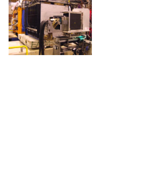
Figure 1: Testbeam setup at CERN, in August 2006. The ECAL is in front, followed by the analogue HCAL and TCMT.

a good resolution at low energy, due to the thin tungsten in the first stack, combined with a good containment of the electromagnetic showers, with an overall thickness of about 20 cm or $24X_{0}$ at normal incidence. To rotate to angles of $10^{\circ}$, $20^{\circ}$, $30^{\circ}$ and $45^{\circ}$ with respect to the beam axis, the three stacks, mechanically separate, are also translated laterally so that the beam still passes through all of them.
The purpose of the testbeam phase is to validate the simulation against a realistic detector, as well as allowing to detect the potential hardware problems. Once the simulation is trusted, full detector studies will lead to the optimisation of the calorimeter for a Particle Flow approach. The test setup at CERN is presented on Figure 1, and is simulated using Mokka [3].
Three drift chambers are used for the tracking at CERN and four at DESY. The ECAL, HCAL [4] and TCMT [5] follow, with the ECAL mounted on a movable stage for angle scans.

2 Summary of the data taken

Eight million triggers were taken at DESY during 14 days in May 2006, for seven beam energies (1, 1.5, 2, 3, 4, 5, 6 GeV), five angles (0^∘, 10^∘, 20^∘, 30^∘, 45^∘) and three positions of the beam on the ECAL front face (center, border and corner of a wafer), with a minimum of 200,000 events per configuration. Six layers were not instrumented: the last eight layers had one dummy slab, one instrumented slab, and two dummy slabs.
The August 2006, CERN beams allowed to take another 8.6 million triggers in ECAL only mode, with the full depth instrumented, for six beam energies between 6 and 45 GeV, and four angles. Pions were taken between 30 and 80 GeV in combination with the HCAL and TCMT. For calibration purposes, 30 million muon events were also taken parasitically to an experiment upstream.
The setup in October 2006 was slightly different, with ECAL and HCAL at 6 cm from each other. 3.8 million triggers were taken with electrons and positrons from 6 to 45 GeV, and 22 million with pions from 6 to 80 GeV. Another 40 million muon events were added for calibration purposes.

3 ECAL Calibration

3.1 Gain Calibration

The current calibration of the ECAL prototype is performed by using a set of $74$ high-statistics muon runs ( $\sim 250,000$ events each), taken during October $2006$ with another experiment upstream, providing a wide spread of the muon beam over the front face of the prototype. The events are triggered with a 1 m² scintillator counter.

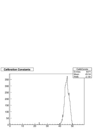
Figure 2: Equivalent ADC value for the energy deposit of 1 MIP for the live cells of the ECAL prototype.

After pedestal substraction (see Section 3.2), the runs are reconstructed using a fixed global noise cut of half a Minimum Ionising Particle (MIP), 1 MIP being estimated to 50 ADC counts by former studies. To reject any remaining noise hits, it is required that the hits of one event form tracks characteristic of a MIP.
The distributions obtained by channel are described by a convolution of a Gaussian and a Landau function. The calibration constant is defined as the most probable value (MPV) of the Landau function, while the standard deviation of the Gaussian defines the noise value for each cell. For 6403 out of the 6480 channels of the prototype, a calibration constant can be obtained via this method without further investigations. The remaining cells show a noise value that is unusually high, and are treated by estimating the additional noise contribution, or by applying the calibration constant from one of their neighbours.
An entire wafer (36 channels) seems to not be fully depleted at the applied voltage of 200V, resulting in a MIP peak at half the normal value. A relative value between the mean MIP signals of the wafer and its neighbours can be estimated, allowing a relative calibration of the cells. 0.14 % of the channels give no output and were considered as dead. The calibration constants for all calibrated channels are histogrammed in Figure 2. The distribution is narrow, with almost all pads in the range 40 to 50 ADC counts per MIP. The small peak at 23.5 corresponds to the single incompletely depleted wafer.

3.2 Pedestal

For all beam tests performed, the data acquisition consists of a fixed sequence of 500 pedestal events, 500 events with charge injection via the calibration chips, and then 20,000 beam events. The pedestal events are used to make a first estimate of the pedestal (mean value) and noise (RMS) per channel.
It has been observed that the pedestals are not necessarily stable, but subject to a random shift affecting all channels of one layer with the same drift. This effect concerns several particular PCBs, is time dependant, and is attributed to the instabilities of the power supplies giving the pedestal lines, which are not isolated. To correct for these instabilities, the pedestals are recalculated on an event by event basis, by discarding all cells recording a signal, and iterating until the RMS of the distribution obtained with the remaining channels is of the order of the expected noise.

3.3 Noise

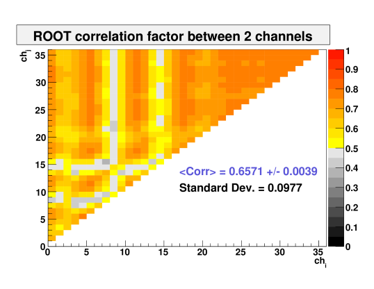
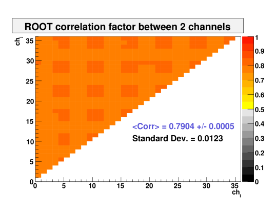
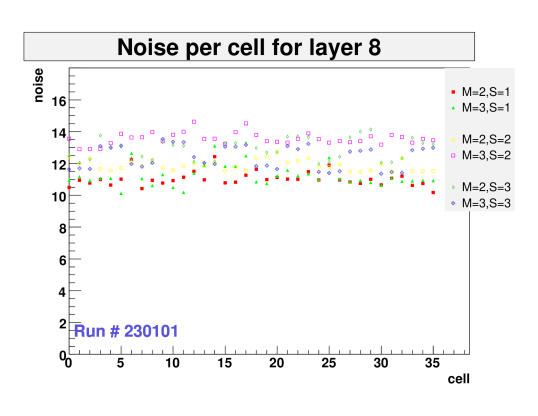
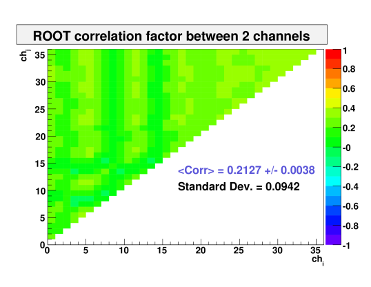
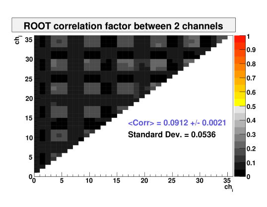
Figure 3: Layer 8, left: module recording a signal, middle: neighbouring wafer, right: mean noise per wafer. Upper row: without corrections, and bottom row: with corrections.

In order to identify coherent noise, the correlation between pairs of channels is calculated in signal events. No clear correlation is seen in an entire PCB, except the one coming from the pedestal drift discussed above. The results are thus shown only on a wafer basis. Figure 3 displays the correlation factors (colour scale) as a function of the channel indices, numbered from 0 to 35, for a particular wafer affected by the pedestal drifts described above, and a run recorded at DESY with an energy of 6 GeV. Channels numbered 0 to 17 and 18 to 35 correspond to two different chips. The corresponding noise level per layer, for all wafers, is also presented in Figure 3, on the right column.
The results before any corrections are shown in the upper row of Figure 3. The left plot represents the module in which the beam was directed. It can be seen that the region with signal shows less correlations, due to the fact that most pixels are discarded in the noise calculation. The middle plots show a neighbouring module, affected only by the global pedestal drift. The difference between these two wafers allows the identification of a crosstalk issue. All the channels of some wafers recording a high signal, like the one presented in Figure 3 on the left, suffer from a pedestal shift towards negative values. This effect does not propagate to the neighbouring wafers. This seems to be random in space and in time, but it is clearly correlated with the intensity of the signal recorded. This effect is not yet understood, but under investigation. In order to correct for the induced correlated noise, the mean and standard deviation are calculated on an event-by-event basis, per wafer, after discarding the signal hits, and iterating over the channels taken into account in the sum. The bottow row on Figure 3 shows the results after all the pedestal corrections described above. The corrections are performing well, bringing the noise back to the normal level of 6 ADC counts. For this particular layer, affected by both problems (i.e. coherent noise on the PCB level due to an instability in the power supply, and crosstalk affecting the wafer recording a high signal), the wafer recording a signal still shows a remaining 20% of correlations. The correlation is however completely removed for wafers affected only by the crosstalk problem, which confirms that the corrections are performing well.

4 Background for physics performance studies: electron selection

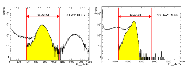
Figure 4: Total ECAL energies for a 3 GeV e^- DESY beam (left) and for 20 GeV at CERN (right), with the energy selection windows. The shaded areas show the effect of the cuts on the shower barycentre (left) and on the Čerenkov counter signal (right).

The selection of the single electron events is loose, in order to avoid bias:

• $E_{cell}\geq 0.6~{}\mbox{MIP}$ removes the noise. The threshold is about five times the average noise measured per cell.

• the total energy recorded in the ECAL, $E_{\mathrm{raw}}$, should be in the range $125<\left(E_{\mathrm{raw}}(\mathrm{MIP})\right)/\left(E_{\mathrm{beam}}(\mathrm{GeV})\right)<375$. $E_{\mathrm{raw}}$ is computed with the three stacks weighted in the ratios 1:2:3, according to the tungsten thickness.

Further cuts are applied to some particular samples: the significant pion content of some high energy electron runs at CERN is reduced by using the threshold Čerenkov counter, whereas the low energy halo coming with some low energy DESY beams is rejected with additional cuts on the shower barycentre. The effect of these two additional cuts is indicated by the shaded regions in Figure 4.

5 Energy Response, Linearity and Resolution

The total response of ECAL is computed by summing the hit energies in the three sections of the detector. If $E_{1}$, $E_{2}$, $E_{3}$ are the recorded energies in the first, second and third stack respectively, the total response is $E_{\mathrm{tot}}=(\alpha_{1}E_{1}+\alpha_{2}E_{2}+\alpha_{3}E_{3})/\beta$. The naïve choice for the weights $(\alpha_{1},\alpha_{2},\alpha_{3})=(1,2,3)$ is generally used. It reflects the relative thicknesses of the tungsten layers in each of the stacks, and hence the relative sampling fractions. However, a weighting scheme optimisation for energy resolution was performed as well, leading to the slightly different values of $(1.1,2.,2.7)$. The normalisation $\beta$ has been arbitrarily fixed to 250 MIP/GeV.

The guard rings create 2 mm non-active inter-wafer gaps, causing non-uniformities in the ECAL response, as illustrated in Figure 5, left, where the mean energy is plotted as a function of the shower barycentre, $(\bar{x},\bar{y})=\sum_{i}(E_{i}x_{i},E_{i}y_{i})/\sum_{i}E_{i}$. Dips in response are clearly visible

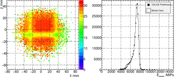
Figure 5: Left: mean ECAL energy as a function of the shower barycentre $(\bar{x},\bar{y})$. Right: total ECAL energy for a 30 GeV $\mathrm{e}^{-}$ beam, for data (points) and Monte Carlo ( open histogram ).

and account for the asymmetric tail on the low side of the distribution of total energy (Figure 5, right), which is reasonably well modelled by the simulation. The correction of these non-uniformities will be discussed in Section 6.

The beam profile, and thus the fraction of beam particles traversing the inter-wafer gaps, depends on the beam energy. Therefore, in order to avoid bias, a cut is applied on the shower barycentre position such as to select showers not affected by the gaps.

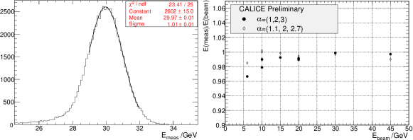
Figure 6: Left: a Gaussian fit to the measured energy, for 30 GeV e^- data. Right: ECAL energy response, divided by beam energy, as a function of beam energy.

To estimate the energy resolution and the mean calorimeter response, the distribution from Figure 6, left, is fitted by a Gaussian in the asymmetric range of $[-\sigma,+2\sigma]$ in order to reduce sensitivity to pion background and to radiative effects upstream of the calorimeter, as well as to any residual influence of the inter-wafer gaps.

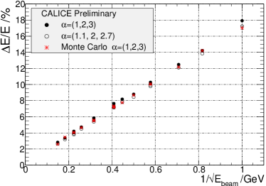
Figure 7: ECAL energy resolution as function of $1/\sqrt{E}$. Two possible weightings of the ECAL stacks are compared.

The ratio of the reconstructed energy to the beam energy, as function of the beam energy is shown in Figure 6, right, for the two choices of weights. Non-linearities are at the $\%$ level. The linearity is somewhat better for the optimised weights.

The energy resolution, similar for both weightings, is shown in Figure 7. The Monte Carlo prediction, with the naïve weights, also shown, is in reasonably good agreement with the data. The resolution can be parametrised, for the naïve choice of weights and, respectively, the optimised one, as

$$\frac{\Delta E}{E}(\%)=\frac{17.7\pm 0.1}{\sqrt{E(\mathrm{GeV})}}\oplus 1.1\pm 0.1\;\;\;\;\;\;\;\;\;\;\;\frac{\Delta E}{E}(\%)=\frac{17.1\pm 0.1}{\sqrt{E(\mathrm{GeV})}}\oplus 0.5\pm 0.2,$$

6 Interwafer gap corrections

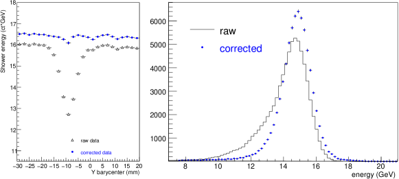
Figure 8: 15 GeV e^-, before (black triangles) and after corrections (blue circles): total energy as function of the shower barycentre $\bar{y}$ (left), and energy distribution (right).

The method used for correcting the interwafer gaps operates at the event level and relies only on the calorimeter information: it parametrises the mean calorimeter response as function of the shower position in the calorimeter and applies subsequently corrective factors for each event according to this parametrisation. It is only geometrical, independent in $\bar{x}$ and $\bar{y}$ and without any explicit dependence on the shower energy.

The impact of the corrections is clearly illustrated in Figure 8, left, where the $y$ scan of ECAL is shown for the raw and, respectively the corrected data. The low energy tail of the energy distribution is greatly reduced (Figure 8, right). The resolution loss when going from the out of gap events to all the events (with corrections applied on the energy) is of the order of 10%. The corrections do not degrade the linearity.

When tracking information is available, it is possible to precisely calculate the shower position within each wafer. Subsequently, the ratio of the active to non-active areas crossed by the shower according to a mean shower shape can be estimated and used to correct the energy recorded in each layer.

7 Shower development

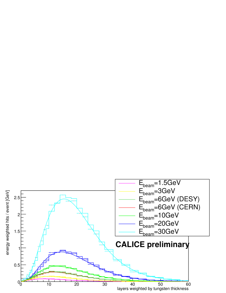
Figure 9: Longitudinal shower profile for the data (points with statistical uncertainties) and Monte Carlo simulation (histogram). The smooth curve is the used parametrisation of the shower profile.

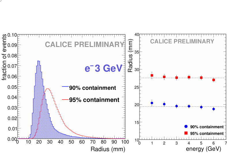
Figure 10: Left: distribution of radii for 90% and 95% signal containment (3 GeV e^-, normal incidence, centre of wafers). Right: radii for 90% and 95% signal containment of e^- as function of the beam energy.

Only events outside the interwafer gaps were used to characterise the longitudinal development of the shower. The mean energy distribution is well fitted by the standard parametrisation, $\gamma(t)=c\,t^{\alpha}\exp(-\beta t)$, where $t$ is the calorimeter depth, $c$ is an overall normalisation, $\alpha$ and $\beta$ are constants (Figure 10). The position of the shower maximum grows logarithmically with the beam energy.

An important issue in the development of a calorimeter is to achieve the smallest possible effective Molière radius, in order to provide the best shower separation. It requires the use of an absorber with a small intrinsic Molière radius ($R_{M}$), but also the minimisation of the gaps between the absorber layers.

Figure 10, left shows the event distribution for 90% and 95% levels of signal containment with respect to the radius. The results for the various energies studied are summarised in Figure 10, right. The points correspond to the peak position of each radius distribution. At 90% (95%) shower containment the corresponding radius, often quoted as 1 $R_{M}$, is about 20 (28) mm.

The geometry of the ECAL prototype, with 2.2 mm thick interlayer gaps leads to an effective Molière radius which is expected to be larger by a factor of about 2 with respect to $R_{M}$ of solid tungsten. The results from the test beam studies are therefore in agreement with expectations. R&D effort towards the use of Si pads with integrated readout is under way and will hopefully lead to a significant decrease of the interlayer gap and therefore of the ECAL effective Molière radius.

8 Spatial and angular resolution of ECAL

The spatial and angular resolution of the ECAL are studied with the DESY data at normal incidence. The shower direction and position at the ECAL front face are constructed on an event-by-event basis using a linear two-parameter chi-square fit to the shower barycentre positions in each layer for the $x$ and $y$ coordinates separately. The correlation matrix is determined from simulations for each beam energy.

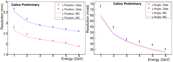
Figure 11: Resolutions in position (left) and angle (right) as a function of the beam energy. The data are shown as points with error bars. The simulation expectation is shown by the continuous line.

The fit results are compared with the position and angle measured by the tracking system. The expected e^- position and direction at ECAL front face is obtained from a linear fit of the drift chambers. Sources of systematic uncertainties as residual misalignement, material modelling, and background rate are estimated for the extrapolation to the ECAL front face.

The ECAL resolution, deconvoluted from the tracking errors, is displayed in Figure 11.

9 Conclusion

The Si/W ECAL prototype was presented, as well as the results of the first beam tests at DESY and CERN during 2006. The prototype calorimeter was further exposed to beam at CERN in summer 2007. Analysis of the data collected is in progress.

References

-
[1]
The CALICE collaboration: calorimeter studies for a future linear collider, 2002.
http://www.ppd.clrc.ac.uk/AnnReps/2004/exp/Calice-317.pdf -
[2]
ECAL mechanical design, available from
http://polywww.in2p3.fr/activities/physique/flc/calice.html -
[3]
Mokka, a detailed Geant4 simulation for the ILC detectors. Available from
http://polywww.in2p3.fr/activities/physique/geant4/tesla/www/mokka/mokka.html - [4] F. Sefkow, “Tile Hadron Calorimeter”, Calorimeter R&D Review, these proceedings.
- [5] D. Chakraborty, “Tail Catcher and Combined Analysis”, these proceedings.