Quantifying Homology Classes II: Localization and Stability

Abstract.

In the companion paper [7], we measured homology classes and computed the optimal homology basis. This paper addresses two related problems, namely, localization and stability. We localize a class with the cycle minimizing a certain objective function. We explore three different objective functions, namely, volume, diameter and radius. We show that it is NP-hard to compute the smallest cycle using the former two. We also prove that the measurement defined in [7] is stable with regard to small changes of the geometry of the concerned space.

1. Introduction

The problem of computing the topological features of a space has recently drawn much attention from researchers in various fields, such as high-dimensional data analysis [3, 14], graphics [12, 5], networks [9] and computational biology [1, 8]. Topological features are often preferable to purely geometric features, as they are more qualitative and global, and tend to be more robust. If the goal is to characterize a space, therefore, features which incorporate topology seem to be good candidates. In this paper, the topological features we use are homology groups over $\mathbb{Z}_{2}$, due to their ease of computation. (Thus, throughout this paper, all the additions are mod 2 additions.)

In the companion paper [7], we addressed the problems of measuring homology classes and finding a concise representation (a homology basis) of the homology group. We defined a size of a homology class as the radius of the smallest geodesic ball carrying the class, using terminology from relative homology. We also computed the optimal homology basis which is the homology basis whose elements’ size have the minimal sum.

This paper addresses two problems that are natural byproducts of the ideas in [7].

Problem 1: Localization.

In the companion paper [7], we localized each class in the optimal homology basis with its localized-cycle, which is the representative cycle carried by the smallest geodesic ball carrying the class. That was necessary for the algorithm to work, but was otherwise not an object of interest. However, the use of localized-cycle suggests an interesting problem: given a natural criterion of the size of a cycle, can we find the smallest cycle in a class? We will see that the companion paper implicitly provided one such criterion, but there are other criteria as well.

The criterion should be deliberately chosen so that the corresponding smallest cycle is concise in not only mathematics but also intuition. Such a cycle is a “well-localized” representative cycle of its class. For example, in Figure 1, the cycles $z_{1}$ and $z_{2}$ are well-localized representatives of their respective homology classes; whereas $z_{3}$ is not.

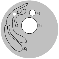
Figure 1. Left: the concerned space is a disk with three holes.
Right: cycles $z_{1}$ and $z_{2}$ are well-localized; $z_{3}$ is not.

This problem of localizing classes with well-localized cycles has potential applications in various field such as high-dimensional data analysis [3, 14], graphics [19, 12, 5], CAD [11], shape study [4], etc. A review of approaches of this problem will be given later in this section.

In this paper, we will look at three such criteria, i.e. the volume, diameter and radius of a cycle. We will show that computing the smallest cycle using the former two are NP-hard, whereas it is polynomial to compute using the latter, which corresponds naturally to the homology class size measure used in the companion paper.

Problem 2: Stability.

We also address another open question suggested by the companion paper. The size measure of homology classes and the optimal homology basis defined in that paper depend on the (discrete) metric on the simplicial complex under consideration. A natural question is: is the measure and the basis stable with respect to small changes in metric? In Section LABEL:sec:stability of this paper, we show that under a suitable definition of stability, the answer is yes. This provides theoretical justification for our work in the companion paper [7].

Restrictions.

Furthermore, as in the companion paper, we make two additional requirements on the solution of the aforementioned problem. First, the solution ought to be computable for topological spaces of arbitrary dimension. Second the solution should not require that the topological space be embedded, for example in a Euclidean space; and if the space is embedded, the solution should not make use of the embedding. These requirements are natural from the theoretical point of view, but may also be justified based on the following applications:

• In machine learning, it is often assumed that the data lives in a manifold whose dimension is much smaller than the dimension of the embedding space.

• In the study of shape, it is common to enrich the shape with other quantities, such as curvature, or color and other physical quantities. This leads to high dimensional manifolds (e.g, 5-7 dimensions) embedded in high dimensional ambient spaces [4].

Related Works.

Using Dijkstra’s shortest path algorithm, Erickson and Whittlesey [13] localized a 1-dimensional homology class with its shortest cycle. They defined the shortest homology basis as the set of $\beta$ linearly independent homology classes, such that lengths of their shortest representative cycles have the minimal sum. They provided a greedy algorithm to localize classes in this basis with their shortest cycles. The authors also showed how the idea carries over to finding the optimal generators of the first fundamental group, though the proof is considerably harder in this case. For completeness, we refer to some related works which compute a single or a set of non-trivial cycles satisfying certain topological and geometrical restrictions on 2-manifolds [12, 16, 6, 10].

Some researchers concentrate on 1-dimensional cycles closely related to handles which are much more meaningful in low dimensional applications such as graphics and CAD. Given a 2-manifold embedded in $S^{3}$, Dey et al. [11] computed these handle-related cycles by computing the deformation retractions of the two components of the the embedding space bounded by the given 2-manifold. Their work facilitates handle detection in real applications. However, the computed 1-cycles are not guaranteed to be geometrically concise. Guskov and Wood [15, 19] detected small handles of a 2-manifold using the Reeb graph of the manifold.

All of the aforementioned works are restricted to low-dimensional manifolds. Zomorodian and Carlsson [20] took a different approach to solving the localization problem for general dimension. Their method starts with a topological space and a cover, which is a set of spaces whose union contains the original space. They computed a homology basis and localized classes of it, using tools from algebraic topology and persistent homology. However, both the quality of the localization and the complexity of the algorithm depend strongly on the choice of cover; there is, as yet, no suggestion of a canonical cover.

Contributions.

We explore the localization problem using different size definitions of a cycle, namely, the volume, diameter and radius.

• We prove that it is NP-hard to localize a class with its smallest cycle in terms of the volume and the diameter, by reduction from MAX-2SAT-B and MCCP, respectively.

• The cycle with the minimal radius is literally the localized-cycle as defined in the companion paper. We show that although it may not be perfectly well-localized, it is a 2-approximation of the cycle with the minimal diameter. A polynomial algorithm to compute this cycle is provided.

For the stability problem, we prove that (1) the size of homology classes and (2) the subgroup filtration computed from the optimal homology basis are both stable with regard to small changes of the geometry of the concerned space.

2. Localization

In this section, we address the localization problem. For ease of computation, we restrict our work to homology groups over $\mathbb{Z}_{2}$ field. Throughout this paper, all the additions are mod 2 additions. When we talk about a $d$-dimensional chain, $c$, we refer to either a collection of $d$-simplices, or a $n_{d}$-dimensional vector over $\mathbb{Z}_{2}$ field, whose non-zero entries corresponds to the included $d$-simplices. Here $n_{d}$ is the total number of $d$-simplices in the given complex. The relevant background in homology can be found in [17].

We formalize the localization problem as a combinatorial optimization problem: Given a simplcial complex $K$, compute the representative cycle of a given homology class minimizing a certain objective function. Formally, given an objective function defined on all the cycles, $\operatorname*{cost}:\mathsf{Z}_{d}(K)\rightarrow\mathbb{R}$, we want to localize a given class with its optimally localized cycle,

$$z_{opt}(h)=\operatorname*{argmin}_{z\in h}\operatorname*{cost}(z).$$

In general, we assume the class $h$ is given by one of its representative cycles, $z_{0}$.

In this paper, we explore three options of the objective function $\operatorname*{cost}(z)$, i.e. the volume, diameter and radius, in the following three subsections.

2.1. Volume

The first choice of the objective function is the volume.

Definition 2.1 (Volume).

The volume of a cycle is the number of its simplices, $\operatorname*{vol}(z)=\operatorname*{card}(z)$.

For example, the volume of a 1-dimensional cycle, a 2-dimensional cycle and a 3-dimensional cycle are the numbers of their edges, triangles and tetrahedra, respectively. A cycle with the smallest volume, denoted as $z_{v}$, is consistent to a “well-localized” cycle in intuition. Its 1-dimensional version, the shortest cycle of a class, has been studied by researchers [13, 19, 11]. However, we prove in Theorem 2.3 that computing $\operatorname*{z_{v}}$ of $h$ is NP-hard.

More generally, we can extend the the volume to be the sum of the weights assigned to simplices of the cycle, given an arbitrary weight function, $w:K\rightarrow\mathbb{R}$, defined on all the simplices of $K$, formally,

$$\operatorname*{vol^{\prime}}(z)=\sum_{\sigma\in z}w(\sigma).$$

Theorem 2.3 implies that computing $\operatorname*{z_{v}}$ using this general volume definition is still NP-hard, because Definition 2.1 is in fact a special case of this general definition (when $w(\sigma)=1$, $\forall\sigma\in K$).

We prove by theorem 2.3 by reduction from the NP-hard problem MAX-2SAT-B [18].

Problem 2.2 (MAX-2SAT-B).

Given $N$ literals, $x_{1}$ to $x_{N}$, and $M$ different clauses, $c_{1}$ to $c_{M}$, each in the form of $(x_{i}\vee x_{j})$, $(\neg x_{i}\vee x_{j})$, $(x_{i}\vee\neg x_{j})$ or $(\neg x_{i}\vee\neg x_{j})$. Each literal appears in at most $B$ clauses. Find an assignment assigning boolean values to all the literals such that the number of satisfied clauses are maximized.

Theorem 2.3.

Computing $\operatorname*{z_{v}}$ for a given $h$ is NP-hard.

Appendix A A Polynomial Algorithm to Compute $\operatorname*{z_{r}}$, the Cycle with the Minimal Radius

In the companion paper, a polynomial algorithm is provided to compute $\operatorname*{z_{r}}$ for classes in the optimal homology basis. We generalize this algorithm to compute $\operatorname*{z_{r}}$ for any given homology class. Please refer to [7] for the correctness of this algorithm.

First, we need the smallest geodesic ball carrying the class we want to localize. The procedure Bmin($K$,$z_{0}$) in Algorithm 1 computes this ball, which uses the procedure Contain-Cycle($K$,$K_{0}$,$z_{0}$) (See Algorithm 2) to detect whether a subcomplex $K_{0}$ carries any cycle of the class to localize.

Algorithm 1 Bmin($K$,$z_{0}$)

0:  Find the smallest geodesic ball, $B_{min}$, carrying any cycle of $h$.

0:  $K$: the given simplicial complex.$z_{0}$: a cycle representing $h$.

0:  $p_{min}$ and $r_{min}$: the center and radius of the computed ball $B_{min}$.

1:  for $p\in\operatorname*{vert}(K)$ do

2:     r=0

3:     repeat

4:        r=r+1

5:     until Contain-Cycle($K$,$B_{p}^{r}$,$z_{0}$)

6:     if $r<r_{min}$ then

7:        $r_{min}=r$

8:        $p_{min}=p$

9:     end if

10:  end for

Algorithm 2 Contain-Cycle($K$,$K_{0}$,$z_{0}$)

0:  test whether $K_{0}$ carries any representative cycle of the class $h=[z_{0}]$.

0:  $K$: the given simplicial complex.$K_{0}$: the subcomplex.$z_{0}$: a cycle representing $h$.

0:  Boolean.

1:  $\hat{Z}_{d}=[\partial_{d+1},z_{0}]$

2:  compute $\partial_{d+1}^{K\backslash K_{0}}$ and $\hat{Z}_{d}^{K\backslash K_{0}}$ by picking up rows of $\partial_{d+1}$ and $\hat{Z}_{d}$ whose corresponding simplices do not belong to $K_{0}$

3:  if  $\operatorname*{rank}(\hat{Z}_{d}^{K\backslash K_{0}})-\operatorname*{rank}(\partial_{d+1}^{K\backslash K_{0}})\neq 1$  then

4:     return true

5:  else

6:     return false

7:  end if

Second, when $B_{min}$ is computed, we compute a cycle of $h$ carried by $B_{min}$ as follows. Solve the equation system $\partial_{d+1}^{K\backslash B_{min}}\gamma+z_{0}^{K\backslash B_{min}}=0$, where $\partial_{d+1}^{K\backslash B_{min}}$ is the matrix formed by the rows of $\partial_{d+1}$ whose corresponding simplices do not belong to $B_{min}$, $z_{0}^{K\backslash B_{min}}$ is the vector formed by the entries of $z_{0}$ whose corresponding simplices do not belong to $B_{min}$. Using the solution $\gamma$, $z_{0}+\partial_{d+1}\gamma$ is a cycle of $h$ carreid by $B_{min}$, and thus is the desired $\operatorname*{z_{r}}$.

References

- [1] P. K. Agarwal, H. Edelsbrunner, J. Harer, and Y. Wang. Extreme elevation on a 2-manifold. Discrete & Computational Geometry, 36:553–572, 2006.
- [2] E. M. Arkin and R. Hassin. Minimum-diameter covering problems. Networks, 36(3):147–155, 2000.
- [3] G. Carlsson. Persistent homology and the analysis of high dimensional data. Symposium on the Geometry of Very Large Data Sets, Febrary 2005. Fields Institute for Research in Mathematical Sciences.
- [4] G. Carlsson, T. Ishkhanov, V. de Silva, and L. J. Guibas. Persistence barcodes for shapes. International Journal of Shape Modeling, 11(2):149–188, 2005.
- [5] C. Carner, M. Jin, X. Gu, and H. Qin. Topology-driven surface mappings with robust feature alignment. In IEEE Visualization, page 69, 2005.
- [6] E. W. Chambers, É. C. de Verdière, J. Erickson, F. Lazarus, and K. Whittlesey. Splitting (complicated) surfaces is hard. In Symposium on Computational Geometry, pages 421–429, 2006.
- [7] C. Chen and D. Freedman. Quantifying homology classes i: Measurement and basis. preprint, submitted to STACS’08, September 2007.
- [8] D. Cohen-Steiner, H. Edelsbrunner, and D. Morozov. Vines and vineyards by updating persistence in linear time. In Symposium on Computational Geometry, pages 119–126, 2006.
- [9] V. de Silva and R. Ghrist. Coverage in sensor networks via persistent homology. Algebraic & Geometric Topology, 2006.
- [10] É. C. de Verdière and J. Erickson. Tightening non-simple paths and cycles on surfaces. In SODA, pages 192–201, 2006.
- [11] T. K. Dey, K. Li, and J. Sun. On computing handle and tunnel loops. In IEEE Proc. NASAGEM, 2007.
- [12] J. Erickson and S. Har-Peled. Optimally cutting a surface into a disk. Discrete & Computational Geometry, 31(1):37–59, 2004.
- [13] J. Erickson and K. Whittlesey. Greedy optimal homotopy and homology generators. In SODA, pages 1038–1046, 2005.
- [14] R. Ghrist. Barcodes: the persistent topology of data. Amer. Math. Soc Current Events Bulletin.
- [15] I. Guskov and Z. J. Wood. Topological noise removal. In Graphics Interface, pages 19–26, 2001.
- [16] M. Kutz. Computing shortest non-trivial cycles on orientable surfaces of bounded genus in almost linear time. In Symposium on Computational Geometry, pages 430–438, 2006.
- [17] J. R. Munkres. Elements of Algebraic Topology. Addison-Wesley, Redwook City, California, 1984.
- [18] C. Papadimitriou and M. Yannakakis. Optimization, approximation, and complexity classes. In STOC ’88: Proceedings of the twentieth annual ACM symposium on Theory of computing, pages 229–234, New York, NY, USA, 1988. ACM Press.
- [19] Z. J. Wood, H. Hoppe, M. Desbrun, and P. Schröder. Removing excess topology from isosurfaces. ACM Trans. Graph., 23(2):190–208, 2004.
- [20] A. Zomorodian and G. Carlsson. Localized homology. In Shape Modeling International, pages 189–198, 2007.