Measuring Volatility Clustering in Stock Markets
Abstract
We propose a novel method to quantify the clustering behavior in a complex time series and apply it to a high-frequency data of the financial markets. We find that regardless of used data sets, all data exhibits the volatility clustering properties, whereas those which filtered the volatility clustering effect by using the GARCH model reduce volatility clustering significantly. The result confirms that our method can measure the volatility clustering effect in financial market.
pacs:
87.10.+e, 89.20.-a, 87.90.+yI Introduction
Recently, financial markets have been known as representatives of complex system, which changes the property of system dynamically according to inflows of various information from outside and interactions between heterogenous agents [1]. In order to understand the complexity of financial market, the methods of interdisciplinary research have been achieving in physics and economics fields. The various stylized facts such as the long-term memory of volatility [2], volatility clustering [3], fat tails [4], multifractality [5, 6] are observed. The obvious properties among the stylized facts are the long-term memory property and clustering effects of the volatility data. In previous studies, clustering behaviors are shown in the return time interval statistics of the climate records [7], medical data, extreme floods [8], and economics [9].
The various models which reflects the volatility clustering effect in order to predict exactly the volatility in the econometrics field are introduced. The autoregressive conditional heteroskedasticity (ARCH) [10] and the generalized autoregressive conditional heteroskedasticity (GARCH) model [11] are the representatives. Namely, the many researches to understand the micro-mechanism of market has been processed. However, the study to quantify the volatility clustering effects is not sufficient yet. If we observe quantitatively the volatility clustering effect in financial markets, we will understand micro phenomena of the market. In this paper, we propose the novel method to quantify the volatility clustering effect in the financial time series.
We find that all data sets analyzed in this paper exhibit the volatility clustering property, whereas the data which filters the volatility clustering effect by the GARCH(1,1) model reduces the degree of volatility clustering significantly.
II DATA and METHODS
II.1 DATA
We investigate quantitatively the volatility clustering behaviors using financial time series including the following market data sets: the 5 minute S&P 500 index from 1995 to 2004 and the 5 minute 28 individual stocks traded in the NYSE with the largest liquidity from 1993 to 2002. The return time series is calculated by the log-difference of high-frequency prices as follows: where represents the stock price at time .
II.2 Method to quantify the volatility clustering
In this subsection, we propose a novel method to quantify the volatility clustering effect. We estimate and analyze quantitatively the volatility clustering effect existed in the financial time series. The process is explained by the following.
Step 1 (The symbolized process): We transfer the return time series to the symbolic data in order to quantify the volatility clustering effect in the financial data using the control parameter, such as the number of bins which is defined as
| (1) |
where is the number of bins. The conditional distribution with statistical significance is calculated by the symbolized process.
Step 2 (Calculating the conditional distribution): We estimate the conditional distribution using the symbolized time series generated in step 1. In other words, the conditional distribution corresponds to the next value of a specific symbol in the symbolic data. Next, we calculate repeatedly the conditional distribution for all symbolic data in the proper regime. The conditional distribution of each symbolic data has a non-trivial property like the conditional value if there is a volatility clustering behavior.
Step 3 (The average value of conditional distribution): The step 3 is the calculation of the average value of the conditional distribution estimated in the step 2. We only consider the conditional distribution of symbolic data in the proper range because the extreme symbolic data are rare. By the average value of the conditional distribution, we observe the volatility clustering effect defined as
| (2) |
where is the element numbers of the conditional distribution in terms of a specific symbol . If the average value is not dependent on the symbolic value , there is no volatility clustering effect because the time series shows the volatility clustering effect only when it has a positive (negative) relation with the positive (negative) values of . Next, we calculate the relation between the specific symbolic values and average values of conditional distribution. In other words, we observe the degree of volatility clustering (DVC) behavior according to the relationship between and . The average value is definded as
where is the degree of volatility clustering effect for the positive and negative cases respectively. When , there is no clustering effect. However, when the value of is nonzero, the degree of volatility clustering effect according to the relative magnitude of is measured. Therefore, we can estimate quantitatively the volatility clustering effect of the financial time series.
III Results
In this section, we present the volatility clustering effect of the financial time series. In order to verify usefulness of the method proposed in this paper, we employ the GARCH(1,1) which reflects the volatility clustering effect.
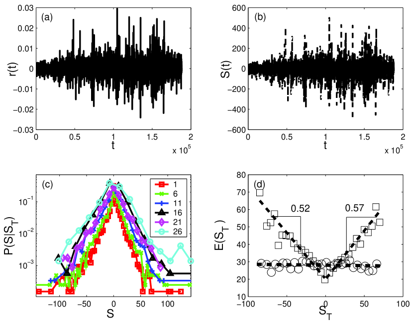
First of all, we apply the novel method to the 5 minute S&P500 index and calculate the degree of volatility clustering. Fig. 1a represents the return time series of the 5 minute S&P500 index and Fig. 1b shows its symbolic time series. We then calculate the conditional distribution of a specific symbol data . Fig. 1c shows the conditional distributions of specific symbols. In Fig. 1c, we find that the width of the conditional distribution increases as the value of symbolic data increases. In other words, the width of the conditional distribution of small symbolic data is relatively narrow than that of large symbolic data. The average value for the conditional distribution regarding specific symbolic data is calculated in order to observe the relationship between specific symbolic values and its conditional distribution. Fig. 1d shows the relationship between specific symbol and average value. Circles and squares of Fig. 1d indicate the original and the surrogate time series respectively. We find that the average values of the conditional distribution for the original time series are positively related to the magnitude of specific symbolic value, and , while those for the shuffled time series is not dependent on the symbolic value . The return time series of the S&P500 index shows the volatility clustering effect, the larger (small) values follow the larger (small) values.
Next, we utilize the GARCH model to verify the usefulness of our method. The GARCH model generates the volatility clustering effect. We create the new time series with the volatility clustering effect removed by the GARCH(1,1) filtering model and estimate the degree of the volatility clustering effect. Fig. 2 displays the degree of the volatility clustering for the 28 individual stocks traded in the NYSE stock market with the largest liquidity. The circles (red), the diamonds (blue), the squares (green), and the triangles (pink) indicate the degree of the volatility clustering for the positive and negative return time series using the original and the GARCH(1,1) filtering data, respectively. In Fig. 2, we find that all the stock return time series, regardless of individual stocks, have the volatility clustering effect, and . However, after eliminating the volatility clustering behavior by the GARCH(1,1) model, the degree of the volatility clustering effect is reduced significantly. This supports that our method to quantify the volatility clustering effect in financial time series is working well.
IV Conclusions
We proposed the novel method to quantify the volatility clustering behavior in financial time series and calculated the degree of the volatility clustering (DVC) using the diverse stock prices. First, we found that all financial data analyzed exhibited the volatility clustering properties, whereas those which are filtered the volatility clustering effect by the GARCH(1,1) model reduced the degree of the volatility clustering effect significantly. This result confirmed that our method calculated the volatility clustering effect in financial time series well. Our method might be applied to elaborate clustering analysis of diverse complex signals including climate, HRV as well as financial time series. Further studies on the volatility clustering will examine to the above systems more extensively.
This work was supported by the Korea Research Foundation funded by the Korean Government (MOEHRD) (KRF-2005-042-B00075), and the MOST/KOSEF to the National Core Research Center for Systems Bio-Dynamics (R15-2004-033), and by the Ministry of Science & Technology through the National Research Laboratory Project, and by the Ministry of Education through the program BK 21.
References
- (1) R. N. Mantegna and H. E. Stanley, An Introduction to Econophysics: Correlation and Complexity in Finance (Cambridge University Press, Cambridge, U.K., 1999); J-P. Bouchaud, M. Potters, Theory of Financial Risk and Derivative Pricing: From Statistical Physics to Risk Management (Cambridge University Press, Cambridge, USA, 2004);
- (2) G. Oh et al., J. Korean Phys. Soc. 48, 197 (2006); Y. Liu et al., Phys. Rev. E 60, 1390 (1999); T. Di Matteo, Journal of Banking & Finance 29, 827 (2005); W. Lo Andrew, Econometrica 59, 1279 (1991).
- (3) I. Giardina et al., Physica A 324, 6 (2003); B. Jacobsen, Journal of Empirical Finance 10, 479 (2003).
- (4) R. N. Mantegna et al., Nature (London) 376, 46 (1995); R. N. Mantegna et al., Nature (London) 383, 587 (1996); V. Plerou et al., Nature (London) 421, 130 (2003); X. Gabaix et al., Nature (London) 423, 267 (2003).
- (5) J. F. Muzy et al., Eur. Phys. J. B 17, 537 (2000); Z. Eisler et al., Physica A 434, 603 (2004); L. Calvet et al., J. of Econometrics 105, 27 (2001); P.C. Ivanov et al., Nature (London) 399, 461 (1999); R. B. Gobindan and H. Kantz, Europhys, Lett. 68, 184 (2004); Y. Ashkenazy et al., Phys. Rev. Lett. 86, 1900 (2001).
- (6) J. F. Muzy et al., Int. J. Bifurcation Chaos Appl. Sci. Eng. 4, 245 (1994).
- (7) A. Bunde et al., Phys. Rev. Lett. 94, 048701 (2005).
- (8) M. Mudelsee et al., Nature (London) 425, 166 (2003).
- (9) K. Yamasaki et al., Proc. Natl. Acad. Sci. 102, 9424 (2005); F. Wang et al., Phys. Rev. E 73, 066128 (2006).
- (10) R. F. Engle, Econometrica 50, 987 (1982).
- (11) T. Bollerslev, J. Econometrics 31, 307 (1986).