Dichroic $f$-sum rule and the orbital magnetization of crystals

Abstract

We consider the magnetic circular dichroism spectrum of a crystal with broken time-reversal symmetry in the electric-dipole approximation. Using the Kubo-Greenwood formula for the absorptive part of the antisymmetric optical conductivity, its frequency integral is recast as a ground-state property. We show that in insulators this quantity is proportional to the circulation of the occupied Wannier orbitals around their centers (more precisely, to the gauge-invariant part thereof). This differs from the net circulation, or ground state orbital magnetization, which has two additional contributions: (i) the remaining Wannier self-rotation, and (ii) the “itinerant” circulation arising from the center-of-mass motion of the Wannier orbitals, both on the surface and in the interior of the sample. Contributions (i) and (ii) are not separately meaningful, since their individual values depend on the particular choice of Wannier functions. Their sum is however gauge-invariant, and can be inferred from a combination of two experiments: a measurement of the magneto-optical spectrum over a sufficiently wide range to evaluate the sum rule, and a gyromagnetic determination of the total orbital magnetization.

I Introduction

Optical sum rules provide a link between excitation spectra and ground-state properties. The best-known example is the $f$-sum rule of atomic physics.Sakurai (1994) It relates the frequency-integrated absorption of linearly polarized light to the number of valence electrons. In this work we consider the analogous result for circularly polarized light. For non-magnetic systems the circular $f$-sum rule is simply the average of the $f$-sum rules for the two linearly-polarized components of the beam, again yielding the total number of electrons. If, however, the system is magnetized, either spontaneously or by an applied field, this is no longer the case; there is a small correction that flips sign when either the magnetization of the sample or the helicity of the incident light is reversed. We are interested in what information this correction to the circular $f$-sum rule provides about the magnetization.

The differential absorption of right- and left-circularly-polarized light by magnetic materials is known as magnetic circular dichroism (MCD). The object of interest in this work can thus be viewed as a “dichroic” $f$-sum rule for the integrated MCD spectrum. Such a sum rule was first derived by Hasegawa and Howard for the special case of a hydrogen atom in a magnetic field.Hasegawa and Howard (1961) They showed that it is proportional to the quantum-mechanical expectation value of the orbital angular momentum operator, i.e., to the orbital moment. It has been assumed that this conclusion generalizes trivially to many-electron systems such as solids.Smith (1976); Thole et al. (1992) This is not so,exp (a) as shown by Oppeneer, who obtained the correct sum rule for that case.Oppeneer (1998) He observed that it yields a quantity that is subtly different from the orbital magnetization ${\bf M}_{\rm orb}$, and should instead be viewed as one of two terms adding up to ${\bf M}_{\rm orb}$.

In a separate development, a rigorous theory of orbital magnetization in crystals was recently formulated.Thonhauser et al. (2005); Xiao et al. (2005); Ceresoli et al. (2006); Shi et al. (2007) Interestingly, it also identifies two separate contributions to ${\bf M}_{\rm orb}$. One key result of the present work is to recast the dichroic $f$-sum rule in the language of this modern theory, elucidating its physical content. Conversely, the sum rule solves an open problem in the theory of Refs. Thonhauser et al., 2005; Xiao et al., 2005; Ceresoli et al., 2006; Shi et al., 2007 as raised explicitly in Ref. Ceresoli et al., 2006: whether the two gauge-invariant contributions to ${\bf M}_{\rm orb}$ identified therein are separately measurable in principle. The present work answers this question in the affirmative.

Although we will mostly focus on crystalline solids, we find it useful to start in Sec. II by discussing the sum rule in the more general context of bounded samples under open boundary conditions. The detailed treatment of periodic crystals is deferred until Sec. III. In both cases, special emphasis will be placed on insulating systems, for which an intuitive real-space picture in terms of occupied Wannier orbitals can be given. We conclude in Sec. IV with a summary and outlook. In Appendices A, B, and C we derive and elaborate on some results quoted in the main text. In particular, Appendix A discusses the relation between the dichroic $f$-sum rule and three other known sum rules.

II Bounded samples

II.1 Preliminaries

In this work we are interested in systems displaying broken time-reversal symmetry in the spatial wavefunctions. A typical example would be a ferromagnet such as iron in which the exchange interaction breaks time-reversal symmetry in the spin channel and this symmetry breaking is then transmitted to the orbital degrees of freedom by the spin-orbit interaction. Other examples include systems in applied magnetic fields, and also certain spinless model Hamiltonians such as the Haldane model.Haldane (1988)

We work in the independent-particle approximation. The interaction with light will be treated in the electric-dipole approximation, valid at not-too-high frequencies. This should be adequate provided that the sum rule saturates before higher-order contributions, such as electric quadrupole and magnetic dipole terms, become significant. The oscillator strength for the transition between one-electron states $n$ and $m$ is

$$f^{(\hat{\boldsymbol{\epsilon}})}_{n\rightarrow m}=\frac{2m_{e}}{\hbar\omega_{mn}}\left|{\langle m|}\hat{\boldsymbol{\epsilon}}\cdot\hat{\bf v}{|n\rangle}\right|^{2}.$$ (1)

This expression, valid for a general polarization $\hat{\boldsymbol{\epsilon}}$ of light, can be derived in the same waySakurai (1994) as the familiar oscillator strength formula for linear polarization $\hat{\boldsymbol{\epsilon}}=\hat{\bf x}$. For light propagating along $\hat{\bf z}$ with circular polarization

$$\hat{\boldsymbol{\epsilon}}_{\pm}=\frac{\hat{\bf x}\pm i\hat{\bf y}}{\sqrt{2}}$$ (2)

(“+” corresponds to positive helicity, or left-circular polarization),

$$f^{(\pm)}_{n\rightarrow m}=\frac{1}{2}\left[f^{\prime}_{nm,xx}+f^{\prime}_{nm,yy}\right]\mp f^{\prime\prime}_{nm,xy},$$ (3)

where we have introduced the matrix

$$f_{nm,\alpha\beta}=\frac{2m_{e}}{\hbar\omega_{mn}}{\langle n|}\hat{v}_{\alpha}{|m\rangle}{\langle m|}\hat{v}_{\beta}{|n\rangle}.$$ (4)

Here $\alpha,\beta$ label Cartesian directions, $\hbar\omega_{mn}={\cal E}_{m}-{\cal E}_{n}$, and $m_{e}$ is the electron mass. Note that the matrix $f=f^{\prime}+if^{\prime\prime}$ is Hermitian in the Cartesian indices. Thus its real and imaginary parts are symmetric and antisymmetric respectively.

According to Eq. (3), the sum of the oscillator strengths for the two circular polarizations $\hat{\boldsymbol{\epsilon}}_{+}$ and $\hat{\boldsymbol{\epsilon}}_{-}$ equals the sum of the oscillator strengths for the two linear polarizations $\hat{\bf x}$ and $\hat{\bf y}$, and is related to $f^{\prime}$. The circular dichroism, i.e., the difference between the two circular oscillator strengths, is given by $f^{\prime\prime}$:

$$f^{\prime\prime}_{nm,xy}=\frac{1}{2}\left[f^{(-)}_{n\rightarrow m}-f^{(+)}_{n\rightarrow m}\right].$$ (5)

Consider now a macroscopic system (e.g., a sample of volume $V$ cut from a bulk crystal) and decompose its optical conductivity $\sigma_{\alpha\beta}(\omega)$ in three different ways: (i) real and imaginary parts, $\sigma^{\prime}$ and $\sigma^{\prime\prime}$; (ii) symmetric and antisymmetric parts, $\sigma_{\rm S}$ and $\sigma_{\rm A}$; (iii) Hermitian and anti-Hermitian parts, $\sigma_{\rm H}$ and $\sigma_{\rm AH}$. Then

$$\sigma_{\rm H}=\sigma^{\prime}_{\rm S}+i\sigma^{\prime\prime}_{\rm A}$$ (6)

and

$$\sigma_{\rm AH}=\sigma^{\prime}_{\rm A}+i\sigma^{\prime\prime}_{\rm S},$$ (7)

where the Cartesian indices and the frequency have been omitted. The properties of $\sigma$ can be summarized by noting that the Hermitian part is dissipative while the anti-Hermitian part is reactive, and the symmetric part is “ordinary” while the antisymmetric part is “dichroic.” At $T=0$ the dissipative (or absorptive) part is

$$\sigma_{\rm H}(\omega)=\frac{\pi e^{2}}{2m_{e}V}\sum_{n}^{\rm occ}\sum_{m}^{\rm empty}f_{nm}\delta(\omega-\omega_{mn}),$$ (8)

where $-e$ is the electron charge. The analog of Eq. (3) in terms of conductivities is

$$\sigma^{(\pm)}_{{\rm abs}}=\frac{1}{2}\left[\sigma^{\prime}_{{\rm S},xx}+\sigma^{\prime}_{{\rm S},yy}\right]\mp\sigma^{\prime\prime}_{{\rm A},xy}.$$ (9)

Thus the difference in absorption between light with negative and positive helicity is given by twice the imaginary part of the antisymmetric optical conductivity,Bennett and Stern (1965)

$$\sigma^{\prime\prime}_{{\rm A},xy}=\frac{1}{2}\left[\sigma^{(-)}_{{\rm abs}}-\sigma^{(+)}_{{\rm abs}}\right].$$ (10)

Like other magneto-optical effects, MCD vanishes for time-reversal-invariant systems. This can be seen from the Onsager relation $\sigma_{\alpha\beta}({\bf H},{\bf M})=\sigma_{\beta\alpha}(-{\bf H},-{\bf M})$, which implies $\sigma_{{\rm A},\alpha\beta}({\bf H}={\bf M}=0)=0$.

II.2 Dichroic $f$-sum rule

With the notation

$$\langle f\rangle\equiv\int_{0}^{\infty}f(\omega)d\omega,$$ (11)

the dichroic $f$-sum rule relates the integrated MCD spectrum $\langle\sigma^{\prime\prime}_{{\rm A},\alpha\beta}\rangle$ to a certain ground-state property of the system. To see how, we begin by expressing $\sigma^{\prime\prime}_{{\rm A},\alpha\beta}(\omega)$ as the imaginary part of the Kubo-Greenwood formula (8). Combining with Eq. (4) and taking the integral,

$$\langle\sigma^{\prime\prime}_{{\rm A},\alpha\beta}\rangle=\frac{\pi e^{2}}{\hbar V}\sum_{n}^{\rm occ}\sum_{m}^{\rm empty}\,{\rm Im}\left(\frac{{\langle n|}\hat{v}_{\alpha}{|m\rangle}{\langle m|}\hat{v}_{\beta}{|n\rangle}}{\omega_{mn}}\right).$$ (12)

Using the identity

$$\frac{{\langle n|}\hat{v}_{\alpha}{|m\rangle}}{\omega_{mn}}=-i{\langle n|}\hat{r}_{\alpha}{|m\rangle}$$ (13)

and defining the projector onto the empty states $\hat{Q}=\sum_{m}^{\rm empty}{|m\rangle}{\langle m|}$,

$$\langle\sigma^{\prime\prime}_{{\rm A},\alpha\beta}\rangle=-\frac{\pi e^{2}}{2\hbar V}\sum_{n}^{\rm occ}{\langle n|}\hat{r}_{\alpha}\hat{Q}\hat{v}_{\beta}{|n\rangle}-(\alpha\leftrightarrow\beta).$$ (14)

Introducing the pseudo-vector $\sigma^{\prime\prime}_{{\rm A},\gamma}=(1/2)\epsilon_{\alpha\beta\gamma}\sigma^{\prime\prime}_{{\rm A},\alpha\beta}$ and $\hat{P}=\sum_{m}^{\rm occ}{|n\rangle}{\langle n|}$, this can be written more concisely as

$$\langle\boldsymbol{\sigma}^{\prime\prime}_{\rm A}\rangle=-\frac{\pi e^{2}}{2\hbar V}{\rm Tr}[\hat{P}\hat{\bf r}\times\hat{Q}\hat{\bf v}].$$ (15)

Eq. (15) is the dichroic $f$-sum rule, also obtained in Ref. Oppeneer, 1998. Using the closure relation $\hat{Q}=\hat{\it 1}-\hat{P}$, it becomes apparent that the right-hand-side depends exclusively on the occupied states, and is closely related to the total (macroscopic) ground-state orbital magnetization ${\bf M}_{\rm orb}=\gamma{\rm Tr}[\hat{P}\hat{\bf r}\times\hat{\bf v}]$, where $\gamma=-(e/2cV)$ in electrostatic units (esu). Writing

$${\bf M}_{\rm orb}={\bf M}_{\rm SR}^{(\rm I)}+\boldsymbol{\Delta}{\bf M},$$ (16)

with

$${\bf M}_{\rm SR}^{(\rm I)}=\gamma{\rm Tr}[\hat{P}\hat{\bf r}\times\hat{Q}\hat{\bf v}]$$ (17)

and

$$\boldsymbol{\Delta}{\bf M}=\gamma{\rm Tr}[\hat{P}\hat{\bf r}\times\hat{P}\hat{\bf v}]$$ (18)

(the notation will be explained shortly), Eq. (15) becomes

$$\langle\boldsymbol{\sigma}^{\prime\prime}_{\rm A}\rangle=\frac{\pi ec}{\hbar}{\bf M}_{\rm SR}^{(\rm I)}.$$ (19)

Hence the sum rule yields an orbital quantity ${\bf M}_{\rm SR}^{(\rm I)}$ with units of magnetization, but differing from the actual orbital magnetization by the remainder $\boldsymbol{\Delta}{\bf M}$.

Two of the three quantities in Eq. (16) are independently measurable. The left-hand side can be determined from gyromagnetic experiments,Kittel (1953); Scott (1962); Huguenin et al. (1971) while ${\bf M}_{\rm SR}^{(\rm I)}$ on the right-hand side is obtainable from magneto-optical experiments via the sum rule. Thus, their difference $\boldsymbol{\Delta}{\bf M}$ can also be determined in principle. However, measuring ${\bf M}_{\rm SR}^{(\rm I)}$ and $\boldsymbol{\Delta}{\bf M}$ independently will be of only limited interest unless some physical meaning can be attached to each of them separately. With this goal in mind we shall now make contact with the recent theory of macroscopic orbital magnetization.

II.3 Relation to the orbital magnetization

The results obtained so far are fairly general. To proceed further we specialize to insulating samples. For the present purposes “insulating” means that the ground state wavefunction can be written as a Slater determinant of well-localized orthonormal molecular orbitals ${|w_{i}\rangle}$, which we will generically refer to as Wannier functions (WFs) even when the sample does not have a crystalline interior.Marzari and Vanderbilt (1997) This definition encompasses a broad range of systems, both macroscopic and microscopic, but it excludes metals and Chern insulators,Thonhauser and Vanderbilt (2006) which are not Wannier-representable in the above sense.

By invariance of the trace, the orbital magnetization can be expressed in the Wannier representation as

$${\bf M}_{\rm orb}=\gamma\sum_{i}^{\rm occ}\,\langle w_{i}|\hat{\bf r}\times\hat{\bf v}|w_{i}\rangle.$$ (20)

In Ref. Thonhauser et al., 2005 this was decomposed asexp (b)

$${\bf M}_{\rm orb}={\bf M}_{\rm SR}+{\bf M}_{\rm IC}$$ (21)

where

$${\bf M}_{\rm SR}=\gamma\sum_{i}^{\rm occ}\,{\langle w_{i}|}(\hat{\bf r}-\overline{\bf r}_{i})\times\hat{\bf v}{|w_{i}\rangle}$$ (22)

arises from the circulation of the occupied WFs around their centers $\overline{\bf r}_{i}=\langle w_{i}|\hat{\bf r}|w_{i}\rangle={\bf r}_{ii}$ (“self-rotation”), while

$${\bf M}_{\rm IC}=\sum_{i}^{\rm occ}\,\overline{\bf r}_{i}\times{\langle w_{i}|}\hat{\bf v}{|w_{i}\rangle}$$ (23)

is the circulation arising from the motion of the centers of mass of the WFs.

It is well known that the WFs of a given system are not uniquely defined; unitary mixing among the WFs is allowed, giving rise to a “gauge freedom” (not to be confused with the freedom to choose the electromagnetic gauge). In practice one deals with this issue by choosing, among the infinitely many possible gauges, a particular one that has certain desirable properties. A common strategy is to work in the gauge that minimizes the quadratic spread of the WFs, producing so-called maximally-localized WFs.Marzari and Vanderbilt (1997) Naturally, any physical observable (e.g., ${\bf M}_{\rm orb}$) is necessarily invariant under a change of gauge. This is unfortunately not the case for the individual terms ${\bf M}_{\rm SR}$ and ${\bf M}_{\rm IC}$ in Eqs. (22)–(23), which turn out to be gauge-dependent. This is to be expected since these quantities do not take the form of traces, unlike those in the decomposition introduced earlier via Eqs. (16)–(18).

The two decompositions (16)–(18) and (21)–(23) are not unrelated, however. To see this, we insert the identity $\hat{\it 1}=\hat{Q}+\hat{P}$ at the location of the cross product in Eq. (22) to obtain

$${\bf M}_{\rm SR}={\bf M}_{\rm SR}^{(\rm I)}+{\bf M}_{\rm SR}^{(\rm II)},$$ (24)

where ${\bf M}_{\rm SR}^{(\rm I)}$ is the quantity defined in Eq. (17) (since ${\langle w_{i}|}\hat{Q}=0$), and

$${\bf M}_{\rm SR}^{(\rm II)} = \gamma\Big{(}{\rm Tr}[\hat{P}\hat{\bf r}\times\hat{P}\hat{\bf v}]-\sum_{i}^{\rm occ}\,\overline{{\bf r}}{{}_{i}}\times\overline{\bf v}_{i}\Big{)}$$ (25)

$$= \gamma\sum_{i,j\not=i}^{\rm occ}\,{\bf r}_{ij}\times{\bf v}_{ji}.$$

In this way we have segregated the gauge-dependence of ${\bf M}_{\rm SR}$ to the term ${\bf M}_{\rm SR}^{(\rm II)}$, isolating a gauge-invariant part ${\bf M}_{\rm SR}^{(\rm I)}$ which turns out to be precisely the quantity defined in Eq. (17) and appearing in the sum rule (19). When the gauge-dependent self-rotation ${\bf M}_{\rm SR}^{(\rm II)}$ is combined with the gauge-dependent itinerant circulation ${\bf M}_{\rm IC}$, it forms the gauge-invariant quantity $\boldsymbol{\Delta}{\bf M}$ of Eq. (18). The relation between the decompositions (16)–(18) and (21)–(23) can be summarized by writing

$${\bf M}_{\rm orb}={\bf M}_{\rm SR}^{(\rm I)}+\underbrace{{\bf M}_{\rm SR}^{(\rm II)}+{\bf M}_{\rm IC}}_{\boldsymbol{\Delta}{\bf M}}.$$ (26)

There is a remarkable parallelism between the decomposition (24) of the Wannier self-rotation (22) and the decompositionMarzari and Vanderbilt (1997)

$$\Omega=\Omega_{\rm I}+\widetilde{\Omega}$$ (27)

of the Wannier spread

$$\Omega=\sum_{i}^{\rm occ}\,{\langle w_{i}|}(\hat{\bf r}-\overline{\bf r}_{i})^{2}{|w_{i}\rangle}$$ (28)

into a gauge-invariant part

$$\Omega_{\rm I}=\sum_{\alpha}\,{\rm Tr}\,[\hat{P}\hat{r}_{\alpha}\hat{Q}\hat{r}_{\alpha}]$$ (29)

and a gauge-dependent part

$$\widetilde{\Omega}=\sum_{i,j\not=i}^{\rm occ}\,|{\bf r}_{ij}|^{2}.$$ (30)

The similarities between Eqs. (17) and (29), and between Eqs. (25) and (30), are striking. Interestingly, the gauge-invariant spread $\Omega_{\rm I}$ is related to the “ordinary” absorption spectrum by a second sum rule, as discussed in Ref. Souza et al., 2000 and Appendix A. In addition, the interpretation of $\Omega_{\rm I}$ as a measure of the quadratic quantum fluctuations, or “quantum spread,” of the many-electron center of massSouza et al. (2000) is mirrored by ${\bf M}_{\rm SR}^{(\rm I)}$ having the meaning of a center-of-mass circulation, as discussed in Appendix B.

First-principles calculations show that for maximally-localized WFs, $\widetilde{\Omega}$ is typically much smaller than $\Omega_{\rm I}$.Marzari and Vanderbilt (1997) Indeed, the minimization of the spread acts precisely to reduce $\widetilde{\Omega}$ as much as possible. In general $\widetilde{\Omega}$ cannot be made to vanish exactly in two or higher dimensions, since the non-commutativity of $\hat{P}\hat{x}\hat{P}$, $\hat{P}\hat{y}\hat{P}$, and $\hat{P}\hat{z}\hat{P}$ implies that the off-diagonal ${\bf r}_{ij}$ cannot all be zero. In practice, however, they can become quite small. According to Eq. (25), ${\bf M}_{\rm SR}^{(\rm II)}$ would also vanish if all off-diagonal ${\bf r}_{ij}$ were precisely zero. Hence we expect the self-rotation of maximally-localized WFs to be dominated by the gauge-invariant part as well.exp (c)

The fact that $\boldsymbol{\Delta}{\bf M}$ is composed of self-rotation and itinerant-circulation parts which are not separately gauge-invariant means that angular momentum can be converted back and forth between ${\bf M}_{\rm SR}$ and ${\bf M}_{\rm IC}$ via gauge transformations. This will be discussed in more detail in Sec. III.4; here we simply note that the two parts are similar in that both originate from the spatial overlap between neighboring WFs. This is evident from the definition of ${\bf M}_{\rm SR}^{(\rm II)}$, and for ${\bf M}_{\rm IC}$ it follows from writing $\overline{\bf v}_{i}$ in terms of the “current donated from one Wannier orbital to its neighbors” as in Ref. Thonhauser et al., 2005. $\boldsymbol{\Delta}{\bf M}$ can therefore be interpreted as an interorbital contribution to ${\bf M}_{\rm orb}$, even though it includes part of the self-rotation, while ${\bf M}_{\rm SR}^{(\rm I)}$ is the purely intraorbital portion. (Similarly, $\Omega_{\rm I}$ and $\widetilde{\Omega}$ are the intraorbital and interorbital parts of the Wannier spread, respectively.)

III Crystalline solids

In this Section we apply the general formalism of Sec. II to crystalline solids, recasting the relevant quantities in the form of Brillouin zone integrals. We start in Sec. III.1 by rederiving the dichroic $f$-sum rule for Bloch electrons. In the remaining subsections we explore the connections between this bulk reformulation and the theory of orbital magnetization in crystals.Thonhauser et al. (2005); Xiao et al. (2005); Ceresoli et al. (2006); Shi et al. (2007)

A somewhat unsatisfying aspect of that theory as developed in Ref. Ceresoli et al., 2006 is the lack of consistency in the way the orbital magnetization was decomposed, in the following sense. One partition (${\bf M}_{\rm orb}={\bf M}_{\rm LC}+{\bf M}_{\rm IC}$ in their notationexp (b)) was made for bounded samples, after which the thermodynamic limit was taken for each term separately. The resulting $k$-space expressions were then combined to form the total ${\bf M}_{\rm orb}$. Finally, working in $k$-space, a different partition (${\bf M}_{\rm orb}=\widetilde{\bf M}_{\rm LC}+\widetilde{\bf M}_{\rm IC}$) was identified whose individual terms were gauge-invariant, unlike those of the original decomposition. In the process, however, the intuitive real-space interpretation of the original decomposition was lost, and the separate meanings of the two terms in the gauge-invariant decomposition was left unclear.

Here, instead, we shall work from the very beginning with the two gauge-invariant terms ${\bf M}_{\rm SR}^{(\rm I)}$ and $\boldsymbol{\Delta}{\bf M}$, which afford a simple real-space interpretation in terms of WFs. They are first identified for fragments with a crystalline interior (crystallites) in Sec. III.2. The thermodynamic limit of each term is then taken, producing the reciprocal-space expressions of Eqs. (46)–(47) (the details of the derivation can be found in Appendix C). Interestingly, we find that our gauge-invariant terms ${\bf M}_{\rm SR}^{(\rm I)}$ and $\boldsymbol{\Delta}{\bf M}$ differ from – but are simply related to – those of the gauge-invariant decomposition of Ref. Ceresoli et al., 2006. In the particular case of an insulator with a single valence band, on the other hand, they reduce exactly to the terms identified in Ref. Xiao et al., 2005, as will be discussed in Sec. III.3. Because the work of Ref. Xiao et al., 2005 is based on a semiclassical picture of wavepacket dynamics, however, it is not easily generalized to a multiband gauge-invariant framework as is done here.

In Eq. (26) of Sec. II the decomposition $\boldsymbol{\Delta}{\bf M}={\bf M}_{\rm SR}^{(\rm II)}+{\bf M}_{\rm IC}$ for insulating systems was obtained by working in the Wannier representation. For insulating crystallites ${\bf M}_{\rm IC}$ can be divided further into a “surface” part ${\bf M}_{\rm IC}^{({\rm surf})}$ and an “interior” part ${\bf M}_{\rm IC}^{({\rm int})}$. The interplay between the resulting three contributions to $\boldsymbol{\Delta}{\bf M}$ will be the focus of the final two subsections. Single-band insulators are discussed in Sec. III.3. The general case of multiband insulators is considered in Sec. III.4, where the gauge-transformation properties of those terms is analyzed.

III.1 Dichroic $f$-sum rule

The first step is to rewrite the Kubo-Greenwood formula (8) in a form appropriate for periodic crystals, where dipole transitions connect valence and conduction Bloch states with the same crystal momentum ${\bf k}$. Eq. (4) becomes, dropping the index ${\bf k}$ for conciseness,

$$f_{nm,\alpha\beta}=-(2m_{e}\omega_{mn}/\hbar)\langle u_{n}|\partial_{\alpha}u_{m}\rangle\langle u_{m}|\partial_{\beta}u_{n}\rangle,$$ (31)

where $\partial_{\alpha}\equiv\partial/\partial k_{\alpha}$ and we have used the relationKing-Smith and Vanderbilt (1993) $v_{nm,\alpha}=\omega_{mn}\langle u_{n}|\partial_{\alpha}u_{m}\rangle$ for $m\not=n$, with ${|u_{n}\rangle}$ a cell-periodic Bloch state. Eq. (8) now reads

$$\sigma_{\rm H}(\omega)=\frac{\pi e^{2}}{2m_{e}}\int\frac{d{\bf k}}{(2\pi)^{3}}\sum_{n}^{\rm occ}\sum_{m}^{\rm empty}f_{nm}\delta(\omega-\omega_{mn}).$$ (32)

Consider the frequency integral of $\sigma_{\rm H}(\omega)$,

$$\langle\sigma_{\rm H}\rangle=\frac{\pi e^{2}}{2m_{e}}\int\frac{d{\bf k}}{(2\pi)^{3}}\,\sum_{n}^{\rm occ}\sum_{m}^{\rm empty}f_{nm}.$$ (33)

The dichroic $f$-sum rule will be obtained from the imaginary part of this complex quantity, while the real part yields the ordinary $f$-sum rule (see Appendix A).

Using Eq. (31) to expand the summation,

$$\sum_{n}^{\rm occ}\sum_{m}^{\rm empty}f_{nm,\alpha\beta}=$$ (34)

$$= -\frac{2m_{e}}{\hbar^{2}}\sum_{n}^{\rm occ}\sum_{m}^{\rm empty}\,\langle u_{n}|\partial_{\alpha}u_{m}\rangle(E_{m}-E_{n})\langle u_{m}|\partial_{\beta}u_{n}\rangle$$

$$= -\frac{2m_{e}}{\hbar^{2}}\sum_{n}^{\rm occ}\sum_{m}^{\rm empty}\,\langle\partial_{\alpha}u_{n}|u_{m}\rangle(E_{n}-E_{m})\langle u_{m}|\partial_{\beta}u_{n}\rangle$$

$$= \frac{2m_{e}}{\hbar^{2}}(g_{{\bf k},\alpha\beta}-h_{{\bf k},\alpha\beta}),$$

where we have introduced a set of notations as follows:

$$b_{{\bf k},\alpha\beta}=\sum_{n}^{\rm occ}\,\langle\widetilde{\partial}_{\alpha}u_{n}|\widetilde{\partial}_{\beta}u_{n}\rangle,$$ (35)

$$g_{{\bf k},\alpha\beta}=\sum_{n}^{\rm occ}\,{\langle\widetilde{\partial}_{\alpha}u_{n}|}\hat{H}{|\widetilde{\partial}_{\beta}u_{n}\rangle},$$ (36)

and

$$h_{{\bf k},\alpha\beta}=\sum_{n}^{\rm occ}\,E_{n}\,\langle\widetilde{\partial}_{\alpha}u_{n}|\widetilde{\partial}_{\beta}u_{n}\rangle.$$ (37)

The symbol $\widetilde{\partial}$ denotes the covariant derivative,Souza et al. (2004); Ceresoli et al. (2006) defined as ${|\widetilde{\partial}_{\alpha}u_{n{\bf k}}\rangle}=\hat{Q}_{\bf k}{|\partial_{\alpha}u_{n{\bf k}}\rangle}$, where $\hat{Q}_{\bf k}=\sum_{m}^{\rm empty}|u_{m{\bf k}}\rangle\langle u_{m{\bf k}}|$. The imaginary part of $b_{{\bf k},\alpha\beta}$ is essentially the Berry curvature while its real part is related to the quantum metric (Appendix C of Ref. Marzari and Vanderbilt, 1997; we discuss the physical content of $b_{{\bf k},\alpha\beta}$ in Appendix A). Quantities $g_{{\bf k},\alpha\beta}$ and $h_{{\bf k},\alpha\beta}$ are similar to $b_{{\bf k},\alpha\beta}$ except that they carry an extra factor of Hamiltonian or energy. Note that $b_{{\bf k},\alpha\beta}$ corresponds to the quantity $f_{{\bf k},\alpha\beta}$ in Ref. Ceresoli et al., 2006, while $g_{{\bf k},\alpha\beta}$ and $h_{{\bf k},\alpha\beta}$ are the same as in that work.

With these definitions Eq. (33) becomes

$$\langle\sigma_{{\rm H},\alpha\beta}\rangle=\frac{\pi e^{2}}{\hbar^{2}}\int\frac{d{\bf k}}{(2\pi)^{3}}\,(g_{{\bf k},\alpha\beta}-h_{{\bf k},\alpha\beta}).$$ (38)

The imaginary part reads, in vector form,

$$\langle\boldsymbol{\sigma}^{\prime\prime}_{\rm A}\rangle=\frac{\pi e^{2}}{\hbar^{2}}\int\frac{d{\bf k}}{(2\pi)^{3}}\,({\bf g}^{\prime\prime}_{\bf k}-{\bf h}^{\prime\prime}_{\bf k}).$$ (39)

This is the dichroic $f$-sum rule in the Bloch representation.

We can now compare this result with the decomposition obtained in Ref. Ceresoli et al., 2006, where the ground-state orbital magnetization was partitioned into two gauge-invariant terms as

$${\bf M}_{\rm orb}=\widetilde{\bf M}_{\rm LC}+\widetilde{\bf M}_{\rm IC}$$ (40)

where

$$\widetilde{\bf M}_{\rm LC}=\frac{e}{\hbar c}\int\frac{d{\bf k}}{(2\pi)^{3}}\,{\bf g}^{\prime\prime}_{\bf k},$$ (41)

$$\widetilde{\bf M}_{\rm IC}=\frac{e}{\hbar c}\int\frac{d{\bf k}}{(2\pi)^{3}}\,{\bf h}^{\prime\prime}_{\bf k}.$$ (42)

We thus arrive at our main result

$$\langle\boldsymbol{\sigma}^{\prime\prime}_{\rm A}\rangle=\frac{\pi ec}{\hbar}\big{(}\widetilde{\bf M}_{\rm LC}-\widetilde{\bf M}_{\rm IC}\big{)}$$ (43)

relating the integrated MCD spectrum to the components of the orbital magnetization. Note that the sum rule is proportional to the difference between the gauge-invariant contributions of Ref. Ceresoli et al., 2006. By independently measuring the sum of $\widetilde{\bf M}_{\rm LC}$ and $\widetilde{\bf M}_{\rm IC}$ via gyromagnetic experimentsKittel (1953) and the difference via the magneto-optical sum rule, the value of each individual term can indeed be measured in principle, resolving an open problem posed in Ref. Ceresoli et al., 2006.

Strictly speaking, Eqs. (40)–(42) as written are valid for conventional insulators only. The generalization to metals and Chern insulators is subtle, but the understanding emerging from Refs. Xiao et al., 2005; Ceresoli et al., 2006; Shi et al., 2007 is that the appropriate generalization is obtained by making the replacements $H\rightarrow H-\mu$ and $E_{n}\rightarrow E_{n}-\mu$ in Eqs. (36) and (37), where $\mu$ is the electron chemical potential. Clearly $g_{\bf k}-h_{\bf k}$, and with it the sum rule (39), are insensitive to these substitutions.exp (d)

Comparing Eqs. (40) and (43) for extended crystals with Eqs. (16) and (19) for bounded samples, it appears plausible that the two partitions (16) and (40) of ${\bf M}_{\rm orb}$ ought to be related by

$${\bf M}_{\rm SR}^{(\rm I)}=\widetilde{\bf M}_{\rm LC}-\widetilde{\bf M}_{\rm IC},$$ (44)

$$\boldsymbol{\Delta}{\bf M}=2\widetilde{\bf M}_{\rm IC},$$ (45)

or explicitly,

$${\bf M}_{\rm SR}^{(\rm I)}=\frac{e}{\hbar c}\int\frac{d{\bf k}}{(2\pi)^{3}}\,({\bf g}^{\prime\prime}_{\bf k}-{\bf h}^{\prime\prime}_{\bf k}),$$ (46)

$$\boldsymbol{\Delta}{\bf M}=\frac{2e}{\hbar c}\int\frac{d{\bf k}}{(2\pi)^{3}}\,{\bf h}^{\prime\prime}_{\bf k}.$$ (47)

The correctness of these identities is demonstrated in Appendix C by taking the thermodynamic limit of results derived in the next subsection.

III.2 The magnetization of an insulating crystallite

To gain a better understanding of the bulk expressions derived in the previous section, we now specialize the results obtained for bounded samples in Sec. II.3 to the case that the sample has a crystalline interior. Working in the Wannier representation, we are then able to establish connections between the $k$-space and Wannier viewpoints and associate a local physical picture with the various terms appearing in the bulk orbital magnetization.

Following Refs. Thonhauser et al., 2005 and Ceresoli et al., 2006, we divide our crystallite into “surface” and “interior” regions. This division is largely arbitrary, and it only needs to satisfy two requirements: (i) the border between the two regions should be placed sufficiently deep inside the sample where the local environment is already crystalline, and (ii) the surface region should occupy a non-extensive volume in the thermodynamic limit. The Wannier orbitals spanning the ground state are assigned to each region. Those in the interior converge exponentially to the bulk WFs ${|{\bf R}n\rangle}$ (${\bf R}$ is a lattice vector), and those on the surface will be denoted by ${|w_{s}\rangle}$.

We first divide the orbital magnetization into self-rotation (SR) and itinerant-circulation (IC) contributions according to Eqs. (21)–(23). In the thermodynamic limit the SR part, which only involves the relative coordinate $\hat{\bf r}-\overline{\bf r}_{i}$, is dominated by the interior region. Invoking translational invariance,

$${\bf M}_{\rm SR}=\gamma_{c}\sum_{n}\,\left[{\langle{\bf 0}n|}\hat{\bf r}\times\hat{\bf v}{|{\bf 0}n\rangle}-\overline{\bf r}_{n}\times\overline{\bf v}_{n}\right],$$ (48)

where $\gamma_{c}=-e/(2cV_{c})$, with $V_{c}$ the cell volume, $\overline{\bf r}_{n}={\langle{\bf 0}n|}\hat{\bf r}{|{\bf 0}n\rangle}$, and $\overline{\bf v}_{n}={\langle{\bf 0}n|}\hat{\bf v}{|{\bf 0}n\rangle}$. Henceforth summations over band-like indices span the valence-band states.

Next we break down the self-rotation as in Eq. (24), setting $\hat{P}=\sum_{\bf R}\sum_{n}\,{|{\bf R}n\rangle}{\langle{\bf R}n|}$:

$${\bf M}_{\rm SR}^{(\rm I)}=\gamma_{c}{\rm Re}\,{\rm tr}_{c}[\hat{P}\hat{\bf r}\times\hat{Q}\hat{\bf v}]$$ (49)

$${\bf M}_{\rm SR}^{(\rm II)} = \gamma_{c}\Big{(}{\rm Re}\,{\rm tr}_{c}[\hat{P}\hat{\bf r}\times\hat{P}\hat{\bf v}]-\sum_{n}\,\overline{\bf r}_{n}\times\overline{\bf v}_{n}\Big{)}$$

$$= \gamma_{c}\sum_{n}\sum_{{\bf R}m\not={\bf 0}n}{\rm Re}\,\big{\{}{\langle{\bf 0}n|}\hat{\bf r}{|{\bf R}m\rangle}\times{\langle{\bf R}m|}\hat{\bf v}{|{\bf 0}n\rangle}\big{\}}.$$

The symbol ${\rm tr}_{c}$ denotes the trace per unit cell. Note that we have taken the real part of the traces explicitly; this was not needed in Eqs. (17) and (25) for bounded samples, where the traces were automatically real.

Now we turn to the IC term (23) in Eq. (21). Unlike ${\bf M}_{\rm SR}$, in the thermodynamic limit it generally has contributions from both interior and surface regions:Thonhauser et al. (2005); Ceresoli et al. (2006)

$${\bf M}_{\rm IC}={\bf M}_{\rm IC}^{(\rm int)}+{\bf M}_{\rm IC}^{(\rm surf)}.$$ (51)

The interior part becomes

$${\bf M}_{\rm IC}^{(\rm int)}=\gamma_{c}\sum_{n}\,\overline{\bf r}_{n}\times\overline{\bf v}_{n}$$ (52)

where it was necessary to use

$$\sum_{n}\,\overline{\bf v}_{n}=0$$ (53)

when exploiting the translational invariance. Eq. (53) expresses the fact that no macroscopic current, or dynamic polarization,Souza et al. (2004) flows through the bulk in a stationary state. Because of this constraint, the quantity (52) necessarily vanishes for insulators with a single valence band. In multiband insulators it takes the form of an intracell itinerant circulation: the WF centers in each cell can have a net circulation while their collective center-of-mass remains at rest.

Finally, the surface contribution is

$${\bf M}_{\rm IC}^{({\rm surf})}=\gamma\sum_{s=1}^{N_{s}}\,\overline{\bf r}_{s}\times\overline{\bf v}_{s}.$$ (54)

It was shown in Refs. Thonhauser et al., 2005 and Ceresoli et al., 2006 that in the thermodynamic limit this can be recast as

$${\bf M}_{\rm IC}^{({\rm surf})}=-{\overline{\gamma}}_{c}\,{\rm Im}\sum_{mn{\bf R}}\,{\bf R}\times{\langle m{\bf 0}|}\hat{\bf r}{|n{\bf R}\rangle}{\langle n{\bf R}|}\hat{H}{|m{\bf 0}\rangle},$$ (55)

where ${\overline{\gamma}}_{c}=\gamma_{c}/\hbar$. This result is remarkable in that it expresses a circulation in the surface region solely in terms of matrix elements between the interior WFs, in a way that does not depend on the precise location of the boundary between the two regions (provided that the boundary satisfies the two criteria mentioned earlier). We emphasize that it holds for crystalline insulators only.

Whereas ${\bf M}_{\rm IC}^{({\rm int})}$ is an intracell-like term, in the bulk form (55) ${\bf M}_{\rm IC}^{({\rm surf})}$ is seen to have an intercell character, vanishing in the “Clausius-Mossotti” limit of zero overlap between WFs belonging to different cells. The assignment of the bulk WFs to specific cells is however not unique, and by making a different choice it is possible to convert between “intracell” ${\bf M}_{\rm IC}^{({\rm int})}$ and “intercell” ${\bf M}_{\rm IC}^{({\rm surf})}$. For this and other reasons to be detailed in Sec. III.4, the interior and surface parts of ${\bf M}_{\rm orb}$ are in general not physically well-defined, even in crystalline insulators. Collecting terms, the full orbital magnetization reads

$${\bf M}_{\rm orb}={\bf M}_{\rm SR}^{(\rm I)}+\underbrace{{\bf M}_{\rm SR}^{(\rm II)}+{\bf M}_{\rm IC}^{(\rm int)}+{\bf M}_{\rm IC}^{(\rm surf)}}_{\boldsymbol{\Delta}{\bf M}},$$ (56)

which is similar to Eq. (26) except that the IC term has been separated into interior and surface parts.

This Wannier-based decomposition of the magnetization of a crystallite follows closely that of Ref. Ceresoli et al., 2006. Two differences are worth noting. First, we have emphasized the distinction between Wannier self-rotation and itinerant circulation. In Ref. Ceresoli et al., 2006 the emphasis was more on the separation between the surface contribution ${\bf M}_{\rm IC}^{({\rm surf})}$ (denoted by ${\bf M}_{\rm IC}$ in that work) and the interior contribution ${\bf M}_{\rm LC}=\gamma_{c}{\rm tr}_{c}[\hat{P}\hat{\bf r}\times\hat{\bf v}]$ containing the net magnetic dipole density of the WFs in a crystalline cell. This “local circulation” includes all of the self-rotation as well as the intracell part of the itinerant circulation. In the present notation the decomposition of Ref. Ceresoli et al., 2006 reads

$${\bf M}_{\rm orb}=\underbrace{{\bf M}_{\rm SR}^{(\rm I)}+{\bf M}_{\rm SR}^{(\rm II)}+{\bf M}_{\rm IC}^{(\rm int)}}_{{\bf M}_{\rm LC}}+{\bf M}_{\rm IC}^{(\rm surf)}.$$ (57)

Note that for one-band insulators ${\bf M}_{\rm IC}^{({\rm int})}=0$, in which case the interior contribution coincides with the self-rotation, and the surface part with the itinerant circulation.Thonhauser et al. (2005) Second, by identifying a gauge-invariant part of the self-rotation, we have been able to organize the four resulting terms into the two gauge-invariant groups indicated in Eq. (56).

The present viewpoint appears to be more useful for arriving at a simple physical picture for the sum rule. It has the additional advantage of being applicable to disordered and microscopic systems, for which the distinction between interior and surface contributions loses meaning.

III.3 One-band insulators

We begin our discussion of ${\bf M}_{\rm orb}$ in insulators with a single valence band by considering the remainder $\boldsymbol{\Delta}{\bf M}$. We saw in Sec. III.2 that, of the three terms into which it is naturally decomposed in the Wannier representation, one of them vanishes if there is only one WF per cell,

$${\bf M}_{\rm IC}^{({\rm int})}=0.$$ (58)

Remarkably, the two surviving terms become identical,

$${\bf M}_{\rm SR}^{(\rm II)}={\bf M}_{\rm IC}^{({\rm surf})}=\frac{\boldsymbol{\Delta}{\bf M}}{2},$$ (59)

and thus individually gauge-invariant. This follows from Eqs. (44)–(45) in the one-band limit. Indeed, the quantities $\widetilde{\bf M}_{\rm LC}$ and $\widetilde{\bf M}_{\rm IC}$ therein were defined in Ref. Ceresoli et al., 2006 in such a way that for one-band insulators they reduce to the quantities ${\bf M}_{\rm LC}={\bf M}_{\rm SR}$ and ${\bf M}_{\rm IC}^{({\rm surf})}$ in Eq. (57). It is then seen that Eqs. (44) and (45) correspond to the first and second equalities in Eq. (59) respectively. We emphasize that Eqs. (58)–(59) only hold for crystalline WFs which respect the full translational symmetry of the crystal. If, for instance, a larger unit cell is used (effectively folding the Brillouin zone and turning the system into a multiband insulator), the additional gauge freedom can be used to construct WFs for which Eqs. (58)–(59) no longer hold.

Consider now the full orbital magnetization. For one-band insulators the reciprocal-space expressions (46)–(47) reduce to

$${\bf M}_{\rm SR}^{(\rm I)}=\frac{e}{2\hbar c}\,{\rm Im}\,\int\frac{d{\bf k}}{(2\pi)^{3}}\,{\langle\partial_{\bf k}u_{\bf k}|}\times(\hat{H}_{\bf k}-E_{\bf k}){|\partial_{\bf k}u_{\bf k}\rangle}$$ (60)

and

$$\boldsymbol{\Delta}{\bf M}=\frac{e}{\hbar c}\,\int\frac{d{\bf k}}{(2\pi)^{3}}\,E_{\bf k}\,{\rm Im}\,{\langle\partial_{\bf k}u_{\bf k}|}\times{|\partial_{\bf k}u_{\bf k}\rangle}.$$ (61)

Their sum ${\bf M}_{\rm orb}$ is given by the right-hand-side of Eq. (60) with $-E_{\bf k}$ replaced by $+E_{\bf k}$, which is the expression originally obtained in Refs. Thonhauser et al., 2005 and Xiao et al., 2005. Moreover, the individual contributions ${\bf M}_{\rm SR}^{(\rm I)}$ and $\boldsymbol{\Delta}{\bf M}$ coincide with those identified in Ref. Xiao et al., 2005. Instead, the derivation of Ref. Thonhauser et al., 2005 leads to the alternative – but, for one-band insulators, also gauge-invariant – partition into the “interior” and “surface” parts ${\bf M}_{\rm LC}={\bf M}_{\rm SR}={\bf M}_{\rm SR}^{(\rm I)}+\boldsymbol{\Delta}{\bf M}/2$ and ${\bf M}_{\rm IC}^{({\rm surf})}=\boldsymbol{\Delta}{\bf M}/2$.

While the individual terms ${\bf M}_{\rm SR}^{(\rm I)}$ and $\boldsymbol{\Delta}{\bf M}$ agree, for single-band insulators, with those of Ref. Xiao et al., 2005, we interpret them somewhat differently here. Eq. (60) of Ref. Xiao et al., 2005 had the meaning of an intrinsic magnetic moment associated with the self-rotation of the carrier wavepackets. According to the present derivation, that term is only part of the Wannier self-rotation. As for Eq. (61), in the derivation of Ref. Xiao et al., 2005 it was seen to arise from a Berry-phase correction to the electronic density of states, and was subsequently claimed to be associated with a boundary current circulation.Xiao et al. (2006) Instead, according to the present viewpoint only half of it originates in the itinerant circulation ${\bf M}_{\rm IC}^{({\rm surf})}$ of the surface WFs, while the other half is ascribed to the remaining self-rotation ${\bf M}_{\rm SR}^{(\rm II)}$ of the WFs in the bulk.

III.4 Gauge transformations for multiband insulators

In multiband insulators all three terms ${\bf M}_{\rm SR}^{(\rm II)}$, ${\bf M}_{\rm IC}^{({\rm int})}$, and ${\bf M}_{\rm IC}^{({\rm surf})}$ can be nonzero. However, their individual values are not physically meaningful, since a gauge transformation can redistribute the total $\boldsymbol{\Delta}{\bf M}$ among them. In particular, it is interesting to consider gauge transformations that shift the location of a WF by a lattice vector.

A general gauge transformation takes the form Marzari and Vanderbilt (1997)

$${|u_{n{\bf k}}\rangle}\rightarrow\sum_{m}\,{|u_{m{\bf k}}\rangle}U_{mn{\bf k}}$$ (62)

where $U_{{\bf k}}$ is an $N_{b}\times N_{b}$ unitary matrix in the band indices. We assume that a transformation of this kind has already been applied to transform from the Hamiltonian eigenstates at each ${\bf k}$ to a set of states that are smooth in ${\bf k}$ from which the WFs are to be constructed. We can then interpose an additional diagonal gauge transformation

$${|u_{n{\bf k}}\rangle}\rightarrow e^{-i{\bf k}\cdot{\bf R}_{n}}{|u_{n{\bf k}}\rangle},$$ (63)

where ${\bf R}_{n}$ is a real-space lattice vector; this has the effect of shifting the location of WF $n$ by ${\bf R}_{n}$. For a one-band insulator, or if ${\bf R}_{n}$ is the same for all bands, this amounts to shifting the choice of the “home” unit cell. However, in the multiband case different WFs can be shifted differently, corresponding to the freedom in choosing which WFs “belong” to the home unit cell.

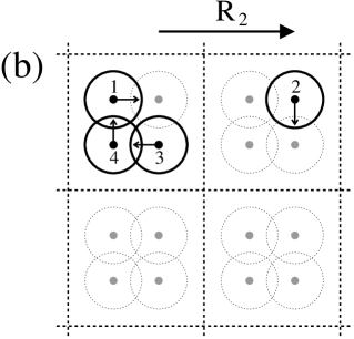
Figure 1: Schematic model of a molecular crystal with one molecule per cell and four WFs per molecule. The range of the orbitals is indicated by the overlapping circles, and their center-of-mass velocities $\overline{\bf v}_{n}$ are denoted by arrows. The two panels show in bold two possible choices of “Wannier basis.”

For example, Fig. 1 shows four cells of a model two-dimensional crystal consisting of “molecular magnets” disposed on a square lattice with lattice constant $a$. Before the transformation (63), the home unit cell contains the four WFs shown in bold in Panel (a). Applying the transformation with ${\bf R}_{2}=a\hat{x}$ and ${\bf R}_{m}=0$ for all other WFs changes the selection of the “basis” of WFs belonging to the home cell to be that shown in Panel (b).

How does this affect the individual terms composing $\boldsymbol{\Delta}{\bf M}$? Clearly the self-rotation (48) is not affected. According to Eq. (52), ${\bf M}_{\rm IC}^{({\rm int})}$ changes by $\gamma_{c}{\bf R}_{2}\times\overline{\bf v}_{2}$. To preserve the overall invariance of $\boldsymbol{\Delta}{\bf M}$ the remaining term ${\bf M}_{\rm IC}^{({\rm surf})}$ must change by an equal and opposite amount. Let us see in more detail how this comes about.

We begin with a formal derivation. The $k$-space expression for ${\bf M}_{\rm IC}^{({\rm surf})}$ is given byCeresoli et al. (2006)

$${\bf M}_{\rm IC}^{({\rm surf})}=\frac{e}{2\hbar c}{\rm Im}\,\sum_{mn}\,\int\frac{d{\bf k}}{(2\pi)^{3}}E_{mn{\bf k}}{\langle\partial_{\bf k}u_{n{\bf k}}|}\times{|\partial_{\bf k}u_{m{\bf k}}\rangle}.$$ (64)

A few steps of algebra show that under the transformation (63) ${\bf M}_{\rm IC}^{({\rm surf})}$ changes by

$$\frac{e}{\hbar c}{\bf R}_{n}\times\sum_{m}\,\int\frac{d{\bf k}}{(2\pi)^{3}}{\rm Re}\,\big{\{}{\langle u_{n}|}\partial_{\bf k}u_{m}\rangle{\langle u_{m}|}\hat{H}_{\bf k}{|u_{n}\rangle}\big{\}}.$$ (65)

Replacing ${\langle u_{n}|}\partial_{\bf k}u_{m}\rangle$ by $-{\langle\partial_{\bf k}u_{n}|}u_{m}\rangle$ allows to identify a term $\hat{P}_{\bf k}\hat{H}_{\bf k}=\hat{H}_{\bf k}$ in the above expression, which becomes

$$-\frac{e}{\hbar c}{\bf R}_{n}\times\int\frac{d{\bf k}}{(2\pi)^{3}}{\rm Re}\big{\{}{\langle u_{n}|}\hat{H}_{\bf k}{|\partial_{\bf k}u_{n}\rangle}\big{\}}.$$ (66)

Comparing with the Wannier velocitySouza et al. (2004)

$$\overline{\bf v}_{n}=-\frac{2V_{c}}{\hbar}\int\frac{d{\bf k}}{(2\pi)^{3}}{\rm Re}\big{\{}{\langle u_{n}|}\hat{H}_{\bf k}{|\partial_{\bf k}u_{n}\rangle}\big{\}}$$ (67)

and setting $n=2$ then produces the desired result $-\gamma_{c}{\bf R}_{2}\times\overline{\bf v}_{2}$ for the change in ${\bf M}_{\rm IC}^{({\rm surf})}$.

Coming back to the example in Fig. 1, the intramolecular orbital overlap gives rise to the nonzero velocities $\overline{\bf v}_{n}$ indicated by the arrows. With the choice of Wannier basis of Panel (a), the collective circulation of the Wannier centers in each cell results in a finite ${\bf M}_{\rm IC}^{({\rm int})}$, while from Eq. (55) ${\bf M}_{\rm IC}^{({\rm surf})}$ vanishes, since there is negligible intercell overlap. When the configuration of Panel (b) is chosen, ${\bf M}_{\rm IC}^{({\rm surf})}$ becomes $-\gamma_{c}{\bf R}_{2}\times\overline{\bf v}_{2}$. From the present viewpoint this nonzero value is made possible by the intramolecular (but now intercell) overlap between the second WF of each cell with WFs one, three, and four from the cell shifted by ${\bf R}_{2}$.

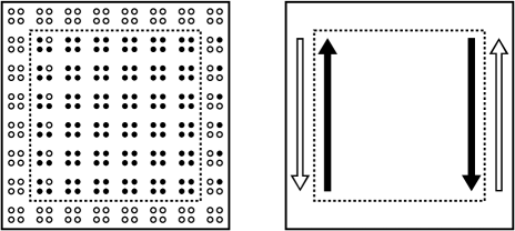
Figure 2: A finite sample cut from the bulk crystal of Fig. 1. With the choice of Wannier basis of Fig. 1(a), “interior” and “surface” WFs lie inside and outside the dashed line respectively; with that of Fig. 1(b), they are denoted by solid and open circles respectively. Right panel: open and solid arrows show the extra “itinerant currents” (${\bf M}_{\rm IC}^{({\rm surf})}$ and ${\bf M}_{\rm IC}^{({\rm int})}$ respectively) associated with the latter choice.

To view ${\bf M}_{\rm IC}^{({\rm surf})}$ as a surface contribution rather than a bulk intercell term, we consider now a finite sample of the same crystal (Fig. 2), which has been divided into surface and interior regions. In deciding which WFs are “interior-like” and which are “surface-like” we shall require that all WFs assigned to the same cell must belong to the same region. If the Wannier basis of Fig. 1(a) is used, the surface region can be chosen to comprise the outermost layer of molecules, so that the border between the two regions is given by the dashed line. The four WFs on each molecule form a unit with some internal IC circulation but zero center-of-mass velocity. The total sample magnetization is the sum of all such internal circulations, which in the large-sample limit is interior-dominated, so that ${\bf M}_{\rm IC}^{({\rm surf})}\rightarrow 0$.

If the Wannier basis of Fig. 1(b) is chosen instead, the upper and lower surface regions are still composed of the outermost layer of molecules. However, the left surface now contains, in addition, one WF from each molecule in the second layer. Those lone surface WFs carry a downward particle “IC current” which extends along the left surface and is indicated by an open arrow on the right panel. A corresponding IC current appears on the right surface, and together they yield ${\bf M}_{\rm IC}^{({\rm surf})}=-(e/2ca)|\overline{\bf v}_{2}|\hat{\bf z}$, which agrees with the result ${\bf M}_{\rm IC}^{({\rm surf})}=-\gamma_{c}{\bf R}_{2}\times\overline{\bf v}_{2}$ found earlier using a purely bulk argument [in this example $\gamma_{c}=-e/(2ca^{2})$]. A change of gauge should not change any physical quantity, such as the actual current flowing on the left surface. Since it appears to change by adding the open arrow, there must be another equal and opposite contribution (the adjacent solid arrow). This contribution is the “interior” IC current carried by the remaining three WFs (filled circles) on the molecules of the second layer.

The situation just described is reminiscent of the “quantum of polarization” in the theory of dielectric polarization,Vanderbilt and King-Smith (1993) where a change of Wannier basis like that leading from Fig. 1(a) to Fig. 1(b) shifts the polarization by a quantum and also changes the surface charge by one electron per surface cell area. This might suggest that the full gauge invariance of the interior and surface parts of ${\bf M}_{\rm orb}$ discussed in Sec. III.3 for single-band insulators becomes, in multiband insulators, a gauge-invariance modulo $\gamma_{c}{\bf R}_{n}\times\overline{\bf v}_{n}$. While true for this particular example, this is generally not so.exp (e) Even for this model it will cease to be true as soon as the molecules start overlapping significantly. When this happens, the value of ${\bf M}_{\rm IC}^{({\rm surf})}$ can be tuned continuously using other types of gauge transformations, e.g., the continuous diagonal transformation

$${|u_{n{\bf k}}\rangle}\rightarrow e^{i\theta_{n{\bf k}}}{|u_{n{\bf k}}\rangle}$$ (68)

with $\theta_{n,{\bf k}+{\bf G}}=\theta_{n{\bf k}}$. This produces a change in ${\bf M}_{\rm IC}^{({\rm surf})}$ given by Eq. (66) with ${\bf R}_{n}$ therein replaced by a factor of $-\partial_{\bf k}\theta_{n{\bf k}}$ in the integrand. Since both $\overline{\bf r}_{n}$ and $\overline{\bf v}_{n}$ remain invariant (the former was shown in Ref. King-Smith and Vanderbilt, 1993 and the latter follows from Eq. (53) together with the fact that all other $\overline{\bf v}_{m}$ are unaffected), so does ${\bf M}_{\rm IC}^{({\rm int})}$. The change in ${\bf M}_{\rm IC}^{({\rm surf})}$ must therefore be absorbed by ${\bf M}_{\rm SR}^{(\rm II)}$.

To summarize, the transformation (63) transfers discrete amounts of itinerant circulation between the interior and surface regions, while the transformation (68) converts continuously between interior self-rotation and surface itinerant circulation. Finally, under the most general transformation (62) all three gauge-dependent terms in Eq. (56) can be affected simultaneously, so that only their sum $\boldsymbol{\Delta}{\bf M}$ is unique and physically meaningful.

IV Summary and outlook

We have presented an exact sum rule for the MCD spectrum, elucidated its physical interpretation, and related it to the recent rigorous formulation of orbital magnetization in crystals. In insulating systems the sum rule probes the gauge-invariant part ${\bf M}_{\rm SR}^{(\rm I)}$ of the self-rotation of the occupied Wannier orbitals. The total orbital magnetization has a second, less obvious contribution $\boldsymbol{\Delta}{\bf M}$, arising from the overlap between neighboring WFs. It comprises both self-rotation (SR) and itinerant-circulation (IC) parts in proportions which depend on the precise choice of WFs, while $\boldsymbol{\Delta}{\bf M}$ itself has a unique value. Although the intuitive interpretation in terms of the occupied WFs is restricted to Wannier-representable systems such as conventional insulators, the terms ${\bf M}_{\rm SR}^{(\rm I)}$ and $\boldsymbol{\Delta}{\bf M}$ are in fact well-defined for all electron systems, including metals and Chern insulators.

The practical importance of the sum rule is that it allows to break down ${\bf M}_{\rm orb}$ into physically meaningful parts, using a combination of gyromagnetic and magneto-optical measurements. This should provide valuable information on the intraorbital (or localized) versus interorbital (or itinerant) character of orbital magnetism. For example, it has been suggested (Ref. Yafet, 1963, Appendix B) that the anomalously large $g$-factors of Bi might be caused by itinerant circulations very much like the ones discussed here. On the basis of the present work it should now be possible to test this conjecture.

In the last decade and a half a sum rule for the X-ray MCD spectrumThole et al. (1992) has been used extensively to obtain site-specific information about orbital magnetism in solids. The resulting orbital moments have been compared with gyromagnetic measurements of ${\bf M}_{\rm orb}$.Chen et al. (1995) If a significant itinerant contribution $\boldsymbol{\Delta}{\bf M}$ is present, one may expect a discrepancy between the XMCD orbital moments and the total ${\bf M}_{\rm orb}$ inferred from gyromagnetics. It would therefore be of great interest to find such systems defying the conventional wisdom about the connection between the MCD spectrum and orbital magnetization.

The ideas discussed in this work should be most relevant for materials displaying appreciable orbital magnetism and, in particular, appreciable interorbital effects which might enhance the ratio $|\boldsymbol{\Delta}{\bf M}/{\bf M}_{\rm SR}^{(\rm I)}|$. These criteria do not favor band ferromagnets. First, their orbital magnetization tends to be relatively small. In the transition metal ferromagnets Fe, Co, and Ni, for example, it accounts for less than 10% of the spontaneous magnetization.Kittel (1953) (For comparison, the field-induced orbital magnetization of the $d$ paramagnetic metals can be as large as the induced spin magnetization. This has been established both from gyromagnetic experimentsHuguenin et al. (1971) and from first-principles calculations.Hjelm et al. (1995)) Secondly, ferromagnetism is favored by narrow bands and localized orbitals, for which interorbital effects are expected to be relatively minor. Finally, the spin-orbit-induced ${\bf M}_{\rm orb}$ of ferromagnets is believed to be an essentially atomic phenomenom largely confined to a small core region close to the nucleus,Solovyev et al. (1998); Solovyev (2005) and one might therefore expect $\boldsymbol{\Delta}{\bf M}$ to be small. Paramagnets and diamagnets, with relatively wide bands (e.g., the $s$-$p$ metals and semiconductors) and additional contributions to ${\bf M}_{\rm orb}$ unrelated to spin-orbit, therefore appear to be more promising candidates. Among ferromagnets, the “zero magnetization ferromagnets,”Adachi and Ino (1999) whose orbital magnetization is so large as to cancel the spin magnetization, might be particularly interesting.

An important direction for future work is to carry out first-principles calculations of ${\bf M}_{\rm SR}^{(\rm I)}$ and $\boldsymbol{\Delta}{\bf M}$ for real materials. Such calculations would test the validity of the assumption that orbital magnetism in solids is atomic-like in nature.Solovyev et al. (1998); Solovyev (2005) While plausible, that assumption was made in the past partly out of practical necessity, since a rigorous bulk definition of ${\bf M}_{\rm orb}$ in terms of the extended Bloch states was not available. Confronting experiment with a full calculation of ${\bf M}_{\rm orb}$ within spin-density functional theory (SDFT), including the itinerant terms, would clarify whether SDFT can adequately describe orbital magnetism in solids, or whether an extended framework (e.g., LSD+U including “orbital polarization” termsSolovyev et al. (1998); Solovyev (2005) or current- and spin-density functional theoryShi et al. (2007)) is needed.

In Appendix A we place the dichroic $f$-sum rule in the broader context of other known sum rules. We note in particular that by taking different inverse-frequency moments, the interband MCD spectrum can be related to two other phenomena resulting from broken time-reversal symmetry, namely the ground state orbital magnetization and the intrinsic anomalous Hall effect. These are generally expected to coexist, and this is indeed the case for ferromagnets, where all three occur spontaneously. In the case of Pauli paramagnets, however, the intrinsic Hall mechanism of Karplus and Luttinger has received little if any attention. On the other hand, it is known that Pauli paramagnets can display a field-induced MCD spectrum.Yaresko et al. (1998); Ebert and Man’kovsky (2003) This raises the question as to what role the Berry curvature may play in their “ordinary” (field-induced) Hall effect. Such a “dissipationless” contribution is undoubtedly present in principle by virtue of the sum rule (75). First-principles calculations of this effect will be presented in a future communication.Yates et al.

To conclude, we have described the orbital magnetization of crystals in terms of localized (${\bf M}_{\rm SR}^{(\rm I)}$) and itinerant ($\boldsymbol{\Delta}{\bf M}$) parts, and shown how to relate them to magneto-optical and gyromagnetic observables. This should allow one to probe more deeply into the nature of magnetism in condensed-matter systems than previously possible.

Appendix A Other sum rules

In this Appendix we derive three additional sum rules for Bloch electrons and discuss their relation to the dichroic $f$-sum rule. All four involve inverse-frequency moments $\langle\omega^{-p}\sigma_{\rm H}\rangle$ [in the notation of Eq. (11)] of the absorption spectrum (6). They are given by $p=0$ and $p=1$, and in each case two sum rules are obtained by taking the real and imaginary parts: one ordinary and the other dichroic, respectively.

We first consider $p=0$. From the imaginary part of Eq. (38) we obtained the dichroic $f$-sum rule (43). To discuss the real part we revert from (38) to the form (33),

$$\langle\sigma^{\prime}_{\rm S,\alpha\beta}\rangle=\frac{\pi e^{2}}{2m_{e}}\int\frac{d{\bf k}}{(2\pi)^{3}}\sum_{n}^{\rm occ}\sum_{m}^{\rm empty}\,f^{\prime}_{nm,\alpha\beta}.$$ (69)

Since $f_{nm,\alpha\beta}=-[f_{mn,\alpha\beta}]^{*}$,

$$\sum_{n}^{\rm occ}\sum_{m}^{\rm empty}\,f^{\prime}_{nm,\alpha\beta} = \sum_{n}^{\rm occ}\sum_{m\not=n}\,f^{\prime}_{nm,\alpha\beta}$$ (70)

$$= \sum_{n}^{\rm occ}\left[\delta_{\alpha\beta}-\left(\frac{m_{e}}{m_{e}^{*}}\right)_{n,\alpha\beta}\right],$$

where the second equality is the effective-mass theorem. Hence we find

$$\langle\sigma^{\prime}_{{\rm S},\alpha\beta}\rangle=\frac{\pi e^{2}}{2m_{e}}\int\frac{d{\bf k}}{(2\pi)^{3}}\sum_{n}^{\rm occ}\,\left[\delta_{\alpha\beta}-\left(\frac{m_{e}}{m_{e}^{*}}\right)_{n,\alpha\beta}\right],$$ (71)

the modified $f$-sum ruleMott and Jones (1936) for the ordinary spectrum.

To obtain the two sum rules for $p=1$ we again start from Eq. (32), but now replace Eq. (34) by

$$\sum_{n}^{\rm occ}\sum_{m}^{\rm empty}\frac{f_{nm,\alpha\beta}}{\omega_{mn}}=\frac{2m_{e}}{\hbar}\,b_{{\bf k},\alpha\beta},$$ (72)

where $b_{n,\alpha\beta}$ was defined in Eq. (35). Thus

$$\langle\omega^{-1}\sigma_{\rm H}\rangle=\frac{\pi e^{2}}{\hbar}\int\frac{d{\bf k}}{(2\pi)^{3}}\,b_{\bf k}.$$ (73)

For the dichroic part, noting that $\boldsymbol{\Omega}_{\bf k}=-2{\bf b}^{\prime\prime}_{\bf k}$ is the Berry curvature summed over the occupied states at ${\bf k}$, and comparing with the “intrinsic” Karplus-Luttinger Hall conductivityYao et al. (2004)

$$\boldsymbol{\sigma}^{\prime}_{\rm A}(\omega=0)=-\frac{e^{2}}{\hbar}\int\frac{d{\bf k}}{(2\pi)^{3}}\,\boldsymbol{\Omega}_{\bf k},$$ (74)

one finds the Hall sum rule,

$$\langle\omega^{-1}\boldsymbol{\sigma}^{\prime\prime}_{\rm A}\rangle=\frac{\pi}{2}\boldsymbol{\sigma}^{\prime}_{\rm A}(\omega=0).$$ (75)

This is the $\omega\rightarrow 0$ limit of the Kramers-Kronig relation for the antisymmetric conductivity.Bennett and Stern (1965) Since only the interband part of the optical conductivity was included on the left-hand-side, the intrinsic dc Hall conductivity was obtained on the right-hand-side. Extrinsic contributions to the latter (e.g., skew scattering) presumably arise from intraband terms in the former.

Finally consider the ordinary (real) part of Eq. (73). The quantity $b^{\prime}_{n,\alpha\beta}$ is the quantum metric.Marzari and Vanderbilt (1997) It is related to the localization tensor $\Lambda_{\alpha\beta}$ of insulators byResta (2002)

$$\Lambda_{\alpha\beta}=\frac{V}{N}\int\frac{d{\bf k}}{(2\pi)^{3}}\,b^{\prime}_{{\bf k},\alpha\beta},$$ (76)

where $N/V$ is the electron density. Hence we recover the electron localization sum ruleSouza et al. (2000)

$$\langle\omega^{-1}\sigma^{\prime}_{\rm S,\alpha\beta}\rangle=\frac{\pi e^{2}N}{\hbar V}\Lambda_{\alpha\beta}.$$ (77)

In summary, we have in Eqs. (38) and (73) two general sum rules for the zero-th and first inverse frequency moments of the optical absorption, respectively. Taking imaginary and real parts of (38) gives the dichroic $f$-sum rule (43) and the modified ordinary $f$-sum rule (71), while taking imaginary and real parts of (73) gives the Hall sum rule (75) and the electron localization sum rule (77).

Besides emerging from a unified formalism, the four sum rules display certain similarities. For instance, it will be shown in Appendix B that the dichroic $f$-sum rule yields the expectation value of the many-electron center-of-mass circulation operator, while the trace of the localization tensor yields the spread of the center-of-mass quantum distribution. Moreover, in a one-particle picture each quantity can be viewed as the gauge-invariant part of the corresponding property (self-rotation or spread) of the Wannier orbitals, as discussed in Sec. II.3 for bounded systems. There is however one important difference between the behavior of the two quantities in the thermodynamic limit. While the center-of-mass circulation remains well-defined for metals, the trace of the localization tensor is only meaningful for insulators, diverging in metals.Souza et al. (2000); Resta (2002) Interestingly, the delocalization of electrons in metals is also responsible for a correction to the $f$-sum rule. Contrary to the canonical $f$-sum rule for atoms,Sakurai (1994) the modified $f$-sum rule (71) does not yield the number density of valence electrons in a metal, due to the presence of the last term on the right-hand-side. This term appears because the Bloch states are extended and do not vanish at infinity.Mott and Jones (1936) The fact that the correction term nevertheless vanishes for insulators is a consequence of the localized nature of insulating many-body wavefunctions in configuration space.Kohn (1968)

We conclude by noting that Eq. (75) provides an extreme example of how sum rules from atomic physics can change qualitatively when applied to extended systems. Indeed, the corresponding sum rule for bound systems produces a vanishing result,exp (f)

$$\langle\omega^{-1}\sigma^{\prime\prime}_{{\rm A},\alpha\beta}\rangle=\frac{\pi e^{2}}{\hbar V}{\rm Im}\,{\rm Tr}[\hat{P}\hat{r}_{\alpha}\hat{Q}\hat{r}_{\beta}]=0.$$ (78)

In contrast, the bulk formula (75) produces for Chern insulators a quantized Hall conductivity, and it also describes the intrinsic anomalous Hall conductivity of ferromagnetic metals.Yao et al. (2004) This apparent contradiction highlights the subtleties associated with the process of taking the thermodynamic limit and switching from open to periodic boundary conditions for non-Wannier-representable systems. Such issues are still not fully resolved in the theory of orbital magnetization. While a general derivation of the bulk formula for ${\bf M}_{\rm orb}$ has been given working from the outset with a periodic crystal,Shi et al. (2007) derivations which start from finite crystallites and take them to the thermodynamic limit (Refs. Thonhauser et al., 2005 and Ceresoli et al., 2006 and Appendix C) are presently restricted to conventional insulators.

Appendix B Dichroic $f$-sum rule and the many-body wavefunction

In the main text we interpreted the dichroic $f$-sum rule, and the associated decomposition (16) of ${\bf M}_{\rm orb}$, in an independent-particle picture based on WFs. It is also possible to relate these quantities directly to properties of the many-electron wavefunction, without invoking any particular single-particle representation. In preparation for that, let us first discuss a one-electron system (e.g., a hydrogen atom in a magnetic field). Its absorption spectrum is composed of sharp lines, and is more conveniently described in terms of an oscillator strength rather than an optical conductivity. Taking the imaginary part of Eq. (4) and using the relation (13) to replace one of the velocity matrix elements,

$$f^{\prime\prime}_{nm,\alpha\beta}=-\frac{m_{e}}{\hbar}\big{[}{\langle n|}\hat{r}_{\alpha}{|m\rangle}{\langle m|}\hat{v}_{\beta}{|n\rangle}-(\alpha\leftrightarrow\beta)\big{]}.$$ (79)

Summing over $m\not=n$ and using the closure relation together with ${\langle n|}\hat{\bf v}{|n\rangle}=0$ one finds, in vector notation,

$$\sum_{m\not=n}\,{\bf f}^{\prime\prime}_{nm}=-\frac{m_{e}}{\hbar}{\langle n|}\hat{\bf r}\times\hat{\bf v}{|n\rangle}.$$ (80)

This is the original dichroic $f$-sum rule of Hasegawa and Howard,Hasegawa and Howard (1961) with the orbital angular momentum appearing on the right-hand-side; in the notation of Sec. II.2 it reads $\langle\boldsymbol{\sigma}^{\prime\prime}_{\rm A}\rangle=(\pi ec/\hbar)\,{\bf M}_{\rm orb}$ (since here $\boldsymbol{\Delta}{\bf M}=0$).

We now generalize the discussion to $N$-electron systems. In this context $\hat{\bf r}=\sum_{i=1}^{N}\hat{\bf r}_{i}$ and $\hat{\bf v}=\sum_{i=1}^{N}\hat{\bf v}_{i}$, and it is crucial to make a distinction between the one-particle operator $\hat{\mathbf{\Lambda}}^{(1)}=\sum_{i=1}^{N}\hat{\bf r}_{i}\times\hat{\bf v}_{i}$ and the two-particle operator $\hat{\mathbf{\Lambda}}^{(2)}=\hat{\bf r}\times\hat{\bf v}$ appearing in Eq. (80), as emphasized in Ref. Kunes and Oppeneer, 2000. The former is related to the electronic angular momentum and orbital magnetization, while the latter is related to a many-electron center-of-mass circulation. (In the classical context, for example, a pair of electrons orbiting 180^∘ out of phase in the same circular orbit would have ${\mathbf{\Lambda}}^{(1)}\neq 0$ but ${\mathbf{\Lambda}}^{(2)}=0$.)

The derivation of the dichroic sum rule for the $N$-electron case proceeds as before, except that the velocity matrix elements in Eq. (4) become ${\bf v}_{nm}={\langle\Psi_{n}|}\hat{\bf v}{|\Psi_{m}\rangle}$, where ${|\Psi_{m}\rangle}$ are now many-body eigenstates. The result is still given by Eq. (80), with ${|n\rangle}$ replaced by ${|\Psi_{n}\rangle}$. Indeed, it is natural to define the many-body generalization of Eq. (17) as

$${\bf M}_{\rm SR}^{(\rm I)}=\gamma{\langle\Psi_{n}|}\hat{\mathbf{\Lambda}}^{(2)}{|\Psi_{m}\rangle}$$ (81)

so that Eq. (19) continues to hold. From this many-body perspective the difference $\boldsymbol{\Delta}{\bf M}$ with respect to the full ${\bf M}_{\rm orb}$ is seen to arise from the cross terms $\sum_{i,j\not=i}^{N}\hat{\bf r}_{i}\times\hat{\bf v}_{j}$ in $\hat{\mathbf{\Lambda}}^{(2)}-\hat{\mathbf{\Lambda}}^{(1)}$.

To recover from (81) the independent-particle expression (17) we specialize to the case where ${|\Psi_{m}\rangle}$ is a single Slater determinant. In second-quantized notation $\hat{\bf r}=\sum_{ij}\,{\bf r}_{ij}c^{\dagger}_{i}c_{j}$, $\hat{\bf v}=\sum_{ij}\,{\bf v}_{ij}c^{\dagger}_{i}c_{j}$, and ${|\Psi_{0}\rangle}=c^{\dagger}_{1}\ldots c^{\dagger}_{N}{|0\rangle}$, where $i$ and $j$ label orthogonal one-particle states. Then Eq. (81) becomes

$${\bf M}_{\rm SR}^{(\rm I)} = \gamma\big{(}{\langle 0|}c_{N}\ldots c_{1}\big{)}\Big{(}\sum_{ij}\,{\bf r}_{ij}c^{\dagger}_{i}c_{j}\Big{)}\times$$ (82)

$$\times \Big{(}\sum_{kl}\,{\bf v}_{kl}c^{\dagger}_{k}c_{l}\Big{)}\big{(}c^{\dagger}_{1}\ldots c^{\dagger}_{N}{|0\rangle}\big{)}.$$ (83)

Terms in which the indices do not pair can immediately be eliminated. Furthermore, pairings of the form ($k=l$, $i=j$) give no contribution, since this leads to $(\sum_{i}^{\rm occ}\,{\bf r}_{ii})\times(\sum_{k}^{\rm occ}\,{\bf v}_{kk})$ which vanishes because $\langle\Psi_{0}|\hat{\bf v}|\Psi_{0}\rangle=0$. The only surviving terms are those with ($j=k$, $i=l$), yielding

$${\bf M}_{\rm SR}^{(\rm I)} = \gamma\sum_{ij}\,{\bf r}_{ij}\times{\bf v}_{ji}\big{(}{\langle\Psi_{0}|}c_{j}c_{j}^{\dagger}\big{)}\big{(}c_{i}^{\dagger}c_{i}{|\Psi_{0}\rangle}\big{)}$$

$$= \gamma\sum_{ij}\,{\bf r}_{ij}\times{\bf v}_{ji}(1-n_{j})n_{i}=\gamma\sum_{i}^{\rm occ}\sum_{j}^{\rm empty}{\bf r}_{ij}\times{\bf v}_{ji},$$

where $n_{i}$ is the state occupancy. Clearly the expression on the right-hand-side is equivalent to that in Eq. (16).

A similar analysis can be made for the other sum rules presented in Appendix A. For example, the counterpart of the Hall sum rule for a bounded many-electron system reads

$$\sum_{m\not=0}\frac{{\bf f}^{\prime\prime}_{0m}}{\omega_{m0}}=-\frac{im_{e}}{\hbar}{\langle\Psi_{0}|}\hat{\bf r}\times\hat{\bf r}{|\Psi_{0}\rangle}=0,$$ (85)

which was termed in Ref. Smith, 1976 the Kuhn sum rule. The independent-particle form (78) can be recovered from (85) along the lines of Eqs. (82)–(B). As for the electron localization sum rule, it yields the second cumulant-moment of the quantum distribution of the many-electron center-of-mass.Souza et al. (2000) In the independent-particle limit this reduces to $\Lambda_{\alpha\beta}=(1/N){\rm Tr}[\hat{P}\hat{r}_{\alpha}\hat{Q}\hat{r}_{\beta}]$, whose trace yields the gauge-invariant WF spread (29). The bulk formula (76) for insulating crystals can be recovered in the thermodynamic limit following the strategy described below for the orbital magnetization.

Appendix C Thermodynamic limit

In this Appendix we start from the expressions (17) and (18) for ${\bf M}_{\rm SR}^{(\rm I)}$ and $\boldsymbol{\Delta}{\bf M}$ of insulating crystallites and, by taking the thermodynamic limit in the Wannier representation, turn them into the reciprocal-space expressions (46) and (47).

Before proceeding, recall that the quantities ${\bf g}_{\bf k}$ and ${\bf h}_{\bf k}$ entering Eqs. (46)–(47) were defined in Eqs. (36)–(37) in the context of the “Hamiltonian gauge” in which $n$ labels a Bloch energy eigenstate. Here, we work with a generalized Wannier representation as in Sec. III.2, where $n$ labels a Wannier function and ${|u_{n{\bf k}}\rangle}$ is the state of Bloch symmetry (generally not an energy eigenstate) constructed from that Wannier function.Marzari and Vanderbilt (1997) The two representations are related by a $k$-dependent unitary rotation as in Eq. (62). Then Eq. (36) remains valid in the present context, since it already takes the form of a trace, while Eq. (37) is now replaced by

$$h_{{\bf k},\alpha\beta}=\sum_{nm}\,E_{nm{\bf k}}{\langle\widetilde{\partial}_{\alpha}u_{m{\bf k}}|}\widetilde{\partial}_{\beta}u_{n{\bf k}}\rangle,$$ (86)

where $E_{nm{\bf k}}={\langle u_{n{\bf k}}|}\hat{H}_{k}{|u_{m{\bf k}}\rangle}$. With ${\bf g}_{\bf k}$ and ${\bf h}_{\bf k}$ written as traces in this way, it is evident that each is a gauge-invariant quantity.Ceresoli et al. (2006)

C.1 Gauge-invariant self-rotation ${\bf M}_{\rm SR}^{(\rm I)}$

For insulating crystallites in the thermodynamic limit, Eq. (17) can be replaced by Eq. (49). Thus we need to establish the equivalence between Eqs. (49) and (46). Using

$${\bf v}=-\frac{i}{\hbar}[\hat{\bf r},\hat{H}]$$ (87)

and specializing to the $z$-component of Eq. (49),

$$M_{{\rm SR},z}^{(\rm I)}=\frac{e}{\hbar cV_{c}}{\rm Im}\,{\rm tr}_{c}[\hat{P}\hat{x}\hat{Q}\hat{H}\hat{Q}\hat{y}-\hat{P}\hat{H}\hat{P}\hat{x}\hat{Q}\hat{y}].$$ (88)

The second term above may be expanded as a trace in the Wannier representation as

$${\rm tr}_{c}[\hat{P}\hat{H}\hat{P}\hat{x}\hat{Q}\hat{y}]=\sum_{\bf R}\sum_{mn}\langle{\bf 0}m|\hat{H}|{\bf R}n\rangle\langle{\bf R}n|\hat{x}\hat{Q}\hat{y}|{\bf 0}m\rangle.$$ (89)

Then using the identities

$$\langle{\bf 0}m|\hat{H}|{\bf R}n\rangle=V_{c}\int\frac{d{\bf k}}{(2\pi)^{3}}\,e^{-i{\bf k}\cdot{\bf R}}E_{mn{\bf k}},$$ (90)

$$\langle{\bf R}n|\hat{x}\hat{Q}\hat{y}|{\bf 0}m\rangle=V_{c}\int\frac{d{\bf k}}{(2\pi)^{3}}\,e^{i{\bf k}\cdot{\bf R}}\langle\widetilde{\partial}_{x}u_{n{\bf k}}|\widetilde{\partial}_{y}u_{m{\bf k}}\rangle,$$ (91)

we obtain

$$\frac{1}{V_{c}}{\rm tr}_{c}[\hat{P}\hat{H}\hat{P}\hat{x}\hat{Q}\hat{y}]=\int\frac{d{\bf k}}{(2\pi)^{3}}\,h_{{\bf k},\alpha\beta}.$$ (92)

Using a similar argument, it follows that

$$\frac{1}{V_{c}}{\rm tr}_{c}[\hat{P}\hat{x}\hat{Q}\hat{H}\hat{Q}\hat{y}]=\int\frac{d{\bf k}}{(2\pi)^{3}}\,g_{{\bf k},\alpha\beta}.$$ (93)

Combining the above two equations with Eq. (88) then yields Eq. (46).

C.2 Gauge-invariant remainder $\boldsymbol{\Delta}{\bf M}$

To take the thermodynamic limit of $\boldsymbol{\Delta}{\bf M}$ we start from Eq. (18) and apply it to a large crystallite to arrive at Eq. (47). Focusing on the $z$-component,

$$(\Delta M)_{z}=\gamma{\rm Tr}[\hat{P}\hat{x}\hat{Q}\hat{v}_{y}]-\gamma{\rm Tr}[\hat{P}\hat{y}\hat{Q}\hat{v}_{x}].$$ (94)

Now use Eq. (87) to obtain

$$(\Delta M)_{z}=-2i\overline{\gamma}{\rm Tr}[\hat{x}\hat{P}\hat{y}\hat{P}\hat{H}\hat{P}-\hat{y}\hat{P}\hat{x}\hat{P}\hat{H}\hat{P}],$$ (95)

where we defined $\overline{\gamma}=\gamma/\hbar$ and replaced $\hat{P}\hat{H}$ by the more symmetrical form $\hat{P}\hat{H}\hat{P}$. Using $-i{\rm Tr}[\hat{\cal O}-{\cal O}^{\dagger}]=2{\rm Im}\,{\rm Tr}[\hat{\cal O}]$, this becomes

$$(\Delta M)_{z}=4\overline{\gamma}{\rm Im}\,{\rm Tr}[\hat{x}\hat{P}\hat{y}(\hat{P}\hat{H}\hat{P})].$$ (96)

At this point we are still considering a bounded sample. To obtain a bulk expression we first need to manipulate Eq. (96) into a form where the unbounded operators $\hat{x}$ and $\hat{y}$ are sandwiched between $\hat{P}$ and $\hat{Q}$, as in Eq. (88). That ensures that ill-defined diagonal position matrix elements between the extended Bloch states do not occur. We will make use of the following rules for finite-dimensional Hermitian matrices $A$, $B$, $C$, and $D$:

$$\mbox{(i)}\,{\rm Im}\,{\rm Tr}[ABCD]={\rm Im}\,{\rm Tr}[DABC]$$ (97)

$$\mbox{(ii)}\,{\rm Im}\,{\rm Tr}[ABCD]=-{\rm Im}\,{\rm Tr}[DCBA]$$ (98)

$$\mbox{(iii)}\,{\rm Im}\,{\rm Tr}[AB]=0$$ (99)

and, if any two of the matrices $A$, $B$, and $C$ commute,

$$\mbox{(iv)}\,{\rm Im}\,{\rm Tr}[ABC]=0.$$ (100)

Rules (i) and (ii) result from elementary properties of the trace. Rule (iii) is a consequence of (i) and (ii), and rule (iv) follows from (iii). Replacing the first $\hat{P}$ in Eq. (96) by $\hat{\it 1}-\hat{Q}$ and applying rule (iv) to the term containing $\hat{\it 1}$ ($[\hat{x},\hat{y}]=0$ and $\hat{P}\hat{H}\hat{P}$ is Hermitian), we obtain

$$(\Delta M)_{z}=-4\overline{\gamma}{\rm Im}\,{\rm Tr}[\hat{P}\hat{H}\hat{P}\hat{x}\hat{Q}\hat{y}],$$ (101)

which has the desired form.

Now we invoke Wannier-representability to write

$${\rm Tr}[\hat{P}\hat{H}\hat{P}\hat{x}\hat{Q}\hat{y}]=\sum_{j}\,\langle w_{j}|\hat{H}\hat{P}(\hat{x}-\overline{x}_{j})\hat{Q}(\hat{y}-\overline{y}_{j})|w_{j}\rangle$$ (102)

(note that $\hat{P}\overline{\bf r}\hat{Q}=0$). Since only the relative coordinate appears, the contribution from the surface orbitals is non-extensive, vanishing in the thermodynamic limit. We are then left with a bulk-like expression:

$${\rm Tr}[\hat{P}\hat{H}\hat{P}\hat{x}\hat{Q}\hat{y}]\rightarrow\sum_{{\bf R}m}\sum_{{\bf R}^{\prime}n}\,\langle{\bf R}m|\hat{H}|{\bf R}^{\prime}n\rangle\langle{\bf R}^{\prime}n|\hat{x}\hat{Q}\hat{y}|{\bf R}m\rangle.$$ (103)

Both matrix elements on the right-hand-side depend on ${\bf R}$ and ${\bf R}^{\prime}$ only through ${\bf R}^{\prime}-{\bf R}$, and therefore, comparing with Eq. (89),

$$\frac{1}{N_{c}}{\rm Tr}[\hat{P}\hat{H}\hat{P}\hat{x}\hat{Q}\hat{y}]\rightarrow{\rm tr}_{c}[\hat{P}\hat{H}\hat{P}\hat{x}\hat{Q}\hat{y}],$$ (104)

where $N_{c}$ is the number of crystalline cells in the sample. Combining Eqs. (92), (101) and (104) one obtains Eq. (47), which concludes the proof.

References

- Sakurai (1994) J. J. Sakurai, Modern Quantum Mechanics (Addison-Wesley, 1994).
- Hasegawa and Howard (1961) H. Hasegawa and R. E. Howard, J. Phys. Chem. Solids 21, 179 (1961).
- Smith (1976) D. Y. Smith, Phys. Rev. B 13, 5303 (1976).
- Thole et al. (1992) B. T. Thole, P. Carra, F. Sette, and G. van der Laan, Phys. Rev. Lett. 68, 1943 (1992).
- exp (a) The many-electron generalization given in Eq. (70) of Ref. Smith, 1976 (and reproduced in Eq. (1) of Ref. Thole et al., 1992) of the Hasegawa-Howard sum rule appears to be incorrect. The angular momentum operator on the right-hand-side should be replaced by its many-body counterpart, as discussed in Appendix B. Moreover, even for the case of a single electron in the presence of an external magnetic field and/or spin-orbit interaction, one must distinguish between the kinetic angular momentum , which is gauge-covariant with respect to the choice of electromagnetic gauge, and the canonical angular momentum , which is not. Here is the (gauge-covariant) kinetic linear momentum, related to the canonical momentum (generator of translations) by ( is the vector potential, is the vector of Pauli matrices, and is the potential energy). If, as in the present work, the gauge-covariant definition of angular momentum is adopted, the second and third terms inside the brackets on the right-hand-side of Eq. (70) of Ref. Smith, 1976 are absorbed into the first term.
- Oppeneer (1998) P. M. Oppeneer, J. Magn. Magn. Mat. 188, 275 (1998).
- Thonhauser et al. (2005) T. Thonhauser, D. Ceresoli, D. Vanderbilt, and R. Resta, Phys. Rev. Lett. 95, 137205 (2005).
- Xiao et al. (2005) D. Xiao, J. Shi, and Q. Niu, Phys. Rev. Lett. 95, 137204 (2005).
- Ceresoli et al. (2006) D. Ceresoli, T. Thonhauser, D. Vanderbilt, and R. Resta, Phys. Rev. B 74, 024408 (2006).
- Shi et al. (2007) J. Shi, G. Vignale, D. Xiao, and Q. Niu, Phys. Rev. Lett. 99, 197202 (2007).
- Haldane (1988) F. D. M. Haldane, Phys. Rev. Lett. 61, 2015 (1988).
- Bennett and Stern (1965) H. S. Bennett and E. A. Stern, Phys. Rev. 137, A448 (1965).
- Kittel (1953) C. Kittel, Introduction to Solid State Physics (Wiley, 1953), 1st ed.
- Scott (1962) G. G. Scott, Rev. Mod. Phys. 34, 102 (1962).
- Huguenin et al. (1971) R. Huguenin, G. P. Pells, and D. N. Baldock, J. Phys. F: Metal Phys. 1, 281 (1971).
- Marzari and Vanderbilt (1997) N. Marzari and D. Vanderbilt, Phys. Rev. B 56, 12847 (1997).
- Thonhauser and Vanderbilt (2006) T. Thonhauser and D. Vanderbilt, Phys. Rev. B 74, 235111 (2006).
- exp (b) The quantity was called in Ref. Thonhauser et al., 2005. One reason for using a different notation here is that in Ref. Ceresoli et al., 2006 was defined (for crystals) in a different way, by replacing the Wannier center in Eq. (22) by the lattice vector labeling the cell to which the WF “belongs.” The two definitions turn out to be equivalent for single-band insulators (the case of interest in Ref. Thonhauser et al., 2005). In Sec. III.2 we discuss the precise relation between our and the of Ref. Ceresoli et al., 2006 in the multiband case.
- Souza et al. (2000) I. Souza, T. Wilkens, and R. M. Martin, Phys. Rev. B 62, 1666 (2000).
- exp (c) However, since the off-diagonal enter the self-rotation as a first power and the spread as a second power, the non-invariant part may play a larger role in the former quantity than in the latter.
- King-Smith and Vanderbilt (1993) R. D. King-Smith and D. Vanderbilt, Phys. Rev. B 47, 1651 (1993).
- Souza et al. (2004) I. Souza, J. Íñiguez, and D. Vanderbilt, Phys. Rev. B 69, 085106 (2004).
- exp (d) For metals the low-frequency part of the absorption spectrum contains intraband (Drude) contributions in addition to the interband absorption. Only the latter was taken into account in the derivation of the dichroic -sum rule for crystals.
- Xiao et al. (2006) D. Xiao, Y. Yao, Z. Fang, and Q. Niu, Phys. Rev. Lett. 97, 026603 (2006).
- Vanderbilt and King-Smith (1993) D. Vanderbilt and R. D. King-Smith, Phys. Rev. B 48, 4442 (1993).
- exp (e) The quantum of polarization can ultimately be traced to the quantization of the charge in a Wannier function. On the contrary, neither the self-rotation nor the center-of-mass velocity of a Wannier function is quantized; these can change continuously under a multiband gauge transformation.
- Yafet (1963) Y. Yafet, Solid State Phys. 14, 1 (1963).
- Chen et al. (1995) C. T. Chen, Y. U. Idzerda, H.-J. Lin, N. V. Smith, G. Meigs, E. Chaban, G. H. Ho, E. Pellegrin, and F. Sette, Phys. Rev. Lett. 75, 152 (1995).
- Hjelm et al. (1995) A. Hjelm, J. Trygg, O. Eriksson, B. Johansson, and J. M. Wills, Int. J. Mod. Phys. B 9, 2735 (1995).
- Solovyev et al. (1998) I. V. Solovyev, A. I. Liechtenstein, and K. Terakura, Phys. Rev. Lett. 80, 5758 (1998).
- Solovyev (2005) I. V. Solovyev, Phys. Rev. Lett. 95, 267205 (2005).
- Adachi and Ino (1999) H. Adachi and H. Ino, Nature 401, 148 (1999).
- Yaresko et al. (1998) A. N. Yaresko, L. Uba, S. Uba, A. Y. Perlov, R. Gontarz, and V. N. Antonov, Phys. Rev. B 58, 7648 (1998).
- Ebert and Man’kovsky (2003) H. Ebert and S. Man’kovsky, Phys. Rev. Lett. 90, 077404 (2003).
- (35) J. R. Yates, D. Vanderbilt, and I. Souza, (in preparation).
- Mott and Jones (1936) N. F. Mott and H. Jones, The Theory of the Properties of Metals and Alloys (Clarendon Press, 1936).
- Yao et al. (2004) Y. Yao, L. Kleinman, A. H. MacDonald, J. Sinova, T. Jungwirth, D.-S. Wang, E. Wang, and Q. Niu, Phys. Rev. Lett. 92, 037204 (2004).
- Resta (2002) R. Resta, J. Phys.: Condens. Matter 14, R625 (2002).
- Kohn (1968) W. Kohn, in Many-Body Physics, edited by C. DeWitt and R. Balian (Gordon and Breach, New York, 1968), p. 351.
- exp (f) To see that the middle expression in Eq. (78) vanishes, write as , note that , , and are all Hermitian, and use Eq. (99).
- Kunes and Oppeneer (2000) J. Kunes and P. M. Oppeneer, Phys. Rev. B 61, 15774 (2000).