The one-dimensional Bose-Fermi-Hubbard model in the heavy-fermion limit

Abstract

We study the phase diagram of the zero-temperature, one-dimensional Bose-Fermi-Hubbard model for fixed fermion density in the limit of small fermionic hopping. This model can be regarded as an instance of a disordered Bose-Hubbard model with dichotomic values of the stochastic variables. Phase boundaries between compressible, incompressible (Mott-insulating) and partially compressible phases are derived analytically within a generalized strong-coupling expansion and numerically using density matrix renormalization group (DMRG) methods. We show that first-order correlations in the partially compressible phases decay exponentially, indicating a glass-type behaviour. Fluctuations within the respective incompressible phases are determined using perturbation theory and are compared to DMRG results.

I Introduction

Ultracold atoms in optical lattices provide an experimentally accessible toolbox for simulating strongly correlated quantum systems lit:Bloch-RMP-2007 ; lit:Jaksch-AnnPhys-2005 ; lit:Jaksch-PRL-1998 ; lit:Fisher-PRB-1988 ; lit:Greiner-Nature-2002 . The interaction of the atoms gives rise to local Hamiltonians on a lattice that can be characterized in their microscopic details. Moreover, by means of mixtures different species, Feshbach resonances, or additional optical lattices, an unprecedented control over system parameters can be achieved. Following first experiments showing a Mott-superfluid phase transition lit:Greiner-Nature-2002 in a bosonic system lit:Fisher-PRB-1988 ; lit:Jaksch-PRL-1998 , a plethora of systems of cold atoms have been studied. This includes mixtures of bosonic and fermionic atoms, – studied in experiments lit:Ketterle-PRL-2002 ; lit:Inguscio-PRL-2004 ; lit:Esslinger-PRL-2006 ; lit:Ospelkaus-PRL-2006 and theory lit:Albus-PRA-2003 ; lit:Lewenstein-PRL-2004 ; lit:Lewenstein-OptComm-2004 ; lit:Cramer-PRL-2004 ; lit:Pazy-PRA-2005 ; lit:Mathey-PRL-2004 ; lit:Demler-PRA-2006 ; lit:Roth-PRA-2004 ; lit:Buechler-PRL-2003 ; lit:Buechler-PRA-2004 ; lit:Pollet-PRL-2006 ; lit:Pollet-condmat-2006 – giving rise to a rich phase diagram and complex physics, including fermion pairing, phase separation, density waves, and supersolids.

Early theoretical studies of the BFHM within mean-field and Gutzwiller decoupling approaches lit:Albus-PRA-2003 ; lit:Lewenstein-OptComm-2004 ; lit:Cramer-PRL-2004 as well as exact numerical diagonalization lit:Roth-PRA-2004 revealed the existence of Mott-insulating (incompressible) phases with incommensurate boson filling. In comparison to the Bose-Hubbard model where the incompressible phases are entirely characterized by the local boson number, the corresponding phases for Bose-Fermi mixtures display a much richer internal structure. A rather complete description of these phases can be obtained using a composite-fermion picture lit:Lewenstein-PRL-2004 , which predicts density waves with integer filling, the formation of composite-fermion domains (phase separation), composite Fermi liquids and BCS-type pairing. The properties of 1D Bose-Fermi mixtures in the compressible phases were analyzed in terms of fermionic polarons using a bosonization approach lit:Mathey-PRL-2004 . In two spatial dimensions the existence of super-solid phases was predicted lit:Buechler-PRL-2003 which is characterized by the simultaneous presence of a density wave and long-range off-diagonal order for the bosons. The persistence of a density wave with noninteger fillings in the compressible phases was shown in lit:Pazy-PRA-2005 . There are also a few exact numerical studies using both quantum Mote-Carlo lit:Pollet-PRL-2006 and DMRG calculations lit:Pollet-condmat-2006 .

In the present work, we consider a Bose-Fermi mixture in a one-dimensional, deep periodic lattice described by the Bose-Fermi-Hubbard model (BFHM). In particular we study the case of small fermionic hopping, where the presence or absence of a fermion at a lattice site results in a dichotomic random alteration of the local potential for the bosons. We show that for this limiting case a rather accurate prediction of the incompressible (Mott-insulating) phases is possible using a generalized strong-coupling approach. To verify this approach we perform numerical simulations using the density-matrix renormalization group (DMRG) lit:Schollwoeck-RMP-2005 . We predict the existence of partially compressible phases and provide numerical evidence that they have a Bose-glass character. Finally we calculate local properties in the incompressible phases and draw conclusions about the validity of effective theories.

II The model

We consider a mixture of ultra-cold, spin polarized fermions and bosons in an optical lattice. In the tight binding limit of a deep lattice potential, the system can be described by the Bose-Fermi Hubbard model lit:Albus-PRA-2003 . We here consider a semi-canonical model, in which the number of fermions is hold constant, but in which we allow for fluctuations of the total number of bosons determined by a chemical potential $\mu$. The corresponding Hamiltonian reads

$$\hat{H} = -J_{B}\sum_{j}\left(\hat{b}^{\dagger}_{j}\hat{b}_{j+1}+\hat{b}^{\dagger}_{j+1}\hat{b}_{j}\right)-\mu\sum_{j}\hat{n}_{j}$$

$$- J_{F}\sum_{j}\left(\hat{c}^{\dagger}_{j}\hat{c}_{j+1}+\hat{c}^{\dagger}_{j+1}\hat{c}_{j}\right)$$

$$+ \frac{U}{2}\sum_{j}\hat{n}_{j}\left(\hat{n}_{j}-1\right)+V\sum_{j}\hat{n}_{j}\hat{m}_{j}.$$

Here, $\hat{c}_{j}$ and $\hat{b}_{j}$ are the annihilation operators of the fermions and bosons at lattice site $j$, respectively, and $\hat{n}_{j}=\hat{b}^{\dagger}_{j}\hat{b}_{j}$, $\hat{m}_{j}=\hat{c}^{\dagger}_{j}\hat{c}_{j}$ the corresponding number operators. The particles can tunnel from one lattice site to a neighboring one, the rate of which is described by $J_{B}$ and $J_{F}$ for bosons and fermions, respectively. $V$ is the on-site interaction strength between the two species, while $U$ accounts for intra-species repulsion of bosons, which will define our energy scale and we set henceforth $U=1$.

Throughout the present work, we will focus on the case of heavy, immobile fermions, i.e., we consider the limit in which $J_{F}=0$ is a good approximation. In this case the effect of the fermions reduces to a dichotomic random potential at site $j$ for the bosons, depending on whether a fermion is at site $j$ or not. This means that the local potential is altered by

$$\delta\mu_{j}=\left\{\begin{array}[]{ll}V,&\text{ if a fermion is present at site $j$,}\\ 0,&\text{ otherwise}.\end{array}\right.$$ (2)

We will systematically investigate to what extent this limit of the Bose-Fermi-Hubbard model can be described as an specific instance of a disordered Bose-Hubbard model,

$$\hat{H} = -J_{B}\sum_{j}\left(\hat{b}^{\dagger}_{j}\hat{b}_{j+1}+\hat{b}^{\dagger}_{j+1}\hat{b}_{j}\right)-\sum_{j}\Bigl{(}\mu-\delta\mu_{j}\Bigr{)}\hat{n}_{j}$$ (3)

$$+ \frac{1}{2}\sum_{j}\hat{n}_{j}\left(\hat{n}_{j}-1\right)$$

We will see that this simple model shows on the one hand important features of the full Bose-Fermi-Hubbard model. On the other hand, we will see that this leads to important qualitative differences to the phase diagram of the disordered Bose-Hubbard model with continuously distributed on-site disorder, as studied in Refs. lit:Fisher-PRB-1988 ; lit:Scholl-EPL-1999 . Depending on the physical situation of interest we will consider two cases of disorder: If the fermionic tunneling is small but sufficiently large such that on the time scales of interest relaxation to the state of total minimum energy is possible, the fermion induced disorder is referred to as being annealed. In this case the ground state is determined by minimization over all possible fermion distributions. If the fermion tunneling is too slow or the temperature too high the disorder is an actually random distribution called quenched.

III Compressible and incompressible phases

In this section we derive the phase diagram of the BFHM with immobile fermions. More specifically, we will approximate the boundaries between compressible and incompressible phases employing a generalization of the familiar strong-coupling expansion lit:Freericks-PRB-1996 to the present case of bosons with a modified potential due to the presence of fermions. This will be compared to the predictions of several instances of mean-field approaches lit:Cramer-PRL-2004 ; lit:Lewenstein-OptComm-2004 . Furthermore, a comparison with numerical results in one spatial dimension obtained by a DMRG computation will be given. Our strong-coupling expansion reveals the existence of novel phases whose character will be discussed in the subsequent section.

III.1 Ultra-deep lattices

We first discuss the simple case of an ultra-deep lattice for the bosons, such that their hopping can be neglected. In this situation where $J_{F}=J_{B}=0$ is a good approximation, the Hamiltonian becomes diagonal in the occupation number basis. This basis will be denoted as $\{|n_{1},\cdots,n_{N}\rangle|m_{1},\cdots,m_{N}\rangle\}$, where $m_{j}=0,1$ denotes the number of fermions at site $j$ and $n_{j}=0,1,...$ the corresponding number of bosons. $N$ labels the total number of lattice sites in the one-dimensional system. The problem of finding the ground state reduces to identifying product states with the lowest energy. By fixing the total number of fermions $N_{F}=N\rho_{F}$, this amounts to minimizing

$$E = \frac{1}{2}\sum_{j}n_{j}(n_{j}-1)-(\mu-V)\sum_{j\in{\cal F}}n_{j}-\mu\sum_{j\in{\cal N}}n_{j}.$$

where ${\cal F}$ denotes the set of $\rho_{F}N=N_{F}$ sites with a fermion and ${\cal N}$ the set of $(1-\rho_{F})N=N-N_{F}$ sites without a fermion, $\rho_{F}$ denoting the fermionic filling factor. The energy is obviously degenerate for all fermion distributions and the ground state is given by an equal mixture of all states with state vectors

$$|\psi_{0}\rangle=\bigotimes_{i\in{\cal F}}|{n}_{1},1\rangle\bigotimes_{j\in{\cal N}}|{n}_{0},0\rangle.$$ (4)

Here,

$${n}_{1}=\max\Bigl{\{}0,[1/2+(\mu-V)]\Bigr{\}},\,{n}_{0}=\max\Bigl{\{}0,[1/2+\mu]\Bigr{\}},$$ (5)

is the local boson number for sites with ($\cal F$) or without (${\cal N}$) a fermion and $[.]$ denotes the closest integer bracket. In other words, the degenerate states with lowest energy will have $\rho_{F}N$ sites with ${n}_{1}$ bosons and one fermion and $N(1-\rho_{F})$ sites with ${n}_{0}$ bosons and no fermion. For the case of zero or unity fermion filling, $\rho_{F}=1$ the situation becomes particularly simple as we encounter the pure Bose-Hubbard model with an effective chemical potential $\mu^{\rm eff}=\mu-V\rho_{F}$.

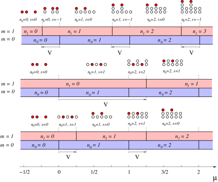
Figure 1: (Color online) Phases of BFHM for $J_{B}=J_{F}=0$ for different inter-species couplings $0<V<1$ (lowest diagram), $1<V<2$ (middle diagram), $-1<V<0$ (upper diagram), and $U=1$. $n$ indicates the number of bosons (empty circles) at the site, $m$ the number of fermions (red filled circles). The horizontal red bars illustrate the boson number $n_{1}$ for sites with a fermion ($m=1$) as function of the chemical potential, the horizontal blue bars correspondingly the boson number $n_{0}$ for sites without a fermion ($m=0$), which is identical to the BHM. The values of $\mu$ where a transition between different boson numbers $n_{0}$ occurs either at sites without a fermion ($m=0$) or with a fermion ($m=1$) are quantum critical points.

Since ${n}_{1}$ and ${n}_{0}$ are integers there are adjacent intervals of $\mu$ where the occupation numbers do not change. In these intervals the system is incompressible, i.e.,

$$\frac{\partial\langle\sum_{j}{\hat{n}}_{j}\rangle}{\partial\mu}=0$$ (6)

and the points between two intervals are quantum critical points. This behavior, illustrated in Fig. 1, is very similar to that of the Bose-Hubbard model except that here the bosons can be incompressible even for non-integer filling $\rho_{B}$ as we have $\rho_{B}={n}_{0}+\rho_{F}({n}_{1}-{n}_{0})$. Following Ref. lit:Lewenstein-PRL-2004 we label the difference ${n}_{0}-{n}_{1}$ in the bosonic number mediated through the presence of a fermion by $s$. The local ground state can either consist of ${n}_{0}$ bosons and no fermion or $n_{1}={n}_{0}-s$ bosons and one fermion. These state vectors will be denoted as $\left|{n}_{0},0\right.\rangle=\left|0\right.\rangle$ and $\left|{n}_{0}-s,1\right.\rangle=\left|1\right.\rangle$. The value of $s$ depends on $\mu$ and $V$ and can be a positive or negative integer. Both these vectors are eigenvectors of the number operator

$$\hat{Q}_{j}=\hat{n}_{j}+s\hat{m}_{j}$$ (7)

with the same integer eigenvalue $n_{0}$ and $\langle\Delta\hat{Q}^{2}_{j}\rangle=0$. Thus incompressible phases have a commensurate number $\hat{Q}$ and can be characterized by the two integers $n_{0}$ and $s$ Since ${n}_{0}$ and ${n}_{1}$ are integers and increase monotonically with $\mu$ , there is a jump in the total number of bosons when moving from one incompressible to the adjacent one. All systems with boson number in between these values are critical and have the same chemical potential since $J_{B}=0$. The average boson number per site in the incompressible phases does not have to be an integer, however. The existence of Mott phases with non-commensurate boson number is a direct consequence of the dichotomic character of the fermion induced disorder. A similar behavior has been predicted for superlattices, which can be considered as dichotomic disorder in the special case of anti-clustering lit:Roth-PRA-2003 ; lit:Buonsante-PRA-2004 . In general Mott-insulating phases with incommensurate boson numbers exist for any disorder distribution that is non-continuous.

III.2 Minimum energy distribution of fermions for small bosonic hopping

In order to understand the physics for disorder due to the presence of fermions we need to discuss the influence of the distribution of fermions to the ground state energy. The energetic degeneracy of different fermion distributions in the incompressible phases is lifted if a small bosonic hopping $J_{B}$ is taken into account. Near the quantum critical points the boson hopping leads to the formation of possibly critical phases with growing extent. We first restrict ourselves to regions where incompressibility is maintained, i.e. sufficiently far away from the critical points.

In order to obtain a qualitative understanding of the effects of a finite bosonic hopping we have performed a numerical perturbation calculation on a small lattice. Fig.2 shows different distributions of 4 fermions over a lattice of 8 sites ordered according to their energy for different parameters in 6th order perturbation.

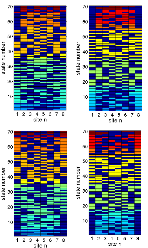
Figure 2: (Color online) Fermion distributions ordered by ground state energy. Blue - lowest energy, red -highest energy for $J_{F}=0$, $J_{B}=0.02$, $U=1$. top: attractive boundary, (i) $V=1.5,{n}_{0}=1,s=1$ i.e. $K_{\rm eff}=-0.002$, and (ii) $V=1.5,{n}_{0}=2,s=1$ i.e. $K_{\rm eff}=0.001$. bottom: repulsive boundary (iii) $V=-1.5,{n}_{0}=0,s=-1$ i.e. $K_{\rm eff}=-0.002$, (iv) $V=-1.5,{n}_{0}=1,s=-1$ i.e. $K_{\rm eff}=0.001$.

One notices that the lowest energy states are either given by fermion distributions with maximum mutual distance (anti-clustered configuration) or minimum mutual distance (clustered configuration) modified by boundary effects. This behavior can in part be explained by the composite fermion picture introduced in lit:Lewenstein-PRL-2004 . The composite fermions are defined for the phase $(n_{0},s)$ by the annihilation operators:

$$\hat{f}_{i} = \sqrt{\frac{(n_{0}-s)!}{n_{0}!}}\,\Bigl{(}\hat{b}_{i}^{\dagger}\Bigr{)}^{s}\,\hat{c}_{i},\qquad\textrm{for}\enspace s\geq 0,$$ (8)

$$\hat{f}_{i} = \sqrt{\frac{n_{0}!}{(n_{0}-s)!}}\,\Bigl{(}\hat{b}_{i}\Bigr{)}^{-s}\,\hat{c}_{i},\quad\enspace\textrm{for}\enspace s<0.$$ (9)

For each $n_{0}$ and $s=1$, the full BFH-Hamiltonian, Eq. (II), with $J_{F}=0$ gives in second order in $J_{B}$ rise to the effective Hamiltonian lit:Lewenstein-PRL-2004

$$\hat{H}_{\rm eff}=K_{\rm eff}\sum_{\langle j,k\rangle}(\hat{f}_{j}^{\dagger}\hat{f}_{j})(\hat{f}_{k}^{\dagger}\hat{f}_{k}),$$ (10)

where $\langle.,.\rangle$ denotes nearest neighbors. Here, as $J_{F}=0$, we find the effective coupling (note that again, $U=1$)

$$K_{\rm eff} = 4J_{B}^{2}\Bigl{[}\frac{n_{0}(n_{0}+1-s)}{1-s+V}+\frac{(n_{0}-s)(n_{0}+1)}{1+s-V}$$ (11)

$$\enspace-n_{0}(n_{0}+1)-(n_{0}-s)(n_{0}+1-s)\Bigr{]}.$$

Composite fermions cannot occupy the same lattice site, but there may be nearest neighbor attraction ($K_{\rm eff}<0$) or repulsion ($K_{\rm eff}>0$). Associating a site with a composite fermion with a spin-up state and a site without a fermion with spin down, Eq. (10) corresponds to the classical Ising model with fixed magnetization and anti-ferromagnetic ($K_{\rm eff}>0$) or ferromagnetic coupling ($K_{\rm eff}<0$).

As a consequence, to this order in perturbation theory, if $K_{\rm eff}<0$, the energy is smallest for fermion distributions that minimize the surface area of sites with and without a fermion (referred to as clustering). In this setting, we can take the fermion distribution to form a block of occupied sites.

The other regime is the one for $K_{\rm eff}>0$. Then, the fermions repel each other, and they form a pattern with maximum number of boundaries for small $J_{B}$, referred to as anti-clustering. That the fermions attain a distribution with maximum distance cannot be explained by the effective model due to its perturbative nature. In all of our numerical simulations using the density matrix renormalization group (DMRG) we found however that a positive $K_{\rm eff}$ always lead to anti-clustering with maximum distance.

The ground state energies of the various fermionic distribution differ only by a small amount which is on the order of $J_{B}^{2}/U$ or even higher powers. Also for temperatures which are still small enough to treat the bosonic system with given disorder as an effective $T=0$ problem, but larger than the energy gap between different fermion distributions, i.e. for $J_{B}(J_{B}/U)^{n}\ll k_{B}T\ll J_{B}$, the various fermion distributions will be equally populated. Thus it seems more natural to consider the case of quenched, random disorder rather than that of annealed disorder.

III.3 Compressible and incompressible phases for finite $J_{B}$

We now discuss the boundaries of the incompressible phases for finite bosonic hopping. To this end we extend the strong coupling expansion of Ref. lit:Freericks-PRB-1996 and complement the results with numerical DMRG simulations. The strong coupling expansion provides a rather accurate description for the Bose-Hubbard model even on a quantitative level.

Let us consider a phase with $(n_{0},s)$ and $N_{F}=\rho_{F}N$ fermions, i.e., a phase with $N_{F}$ sites containing $n_{0}-s$ bosons and a fermion and $N-N_{F}$ sites with $n_{0}$ bosons. The ground state vector for $J_{B}=0$ is then found to be

$$\bigl{|}\psi_{0}\bigr{\rangle}=\bigotimes_{j\in{\cal F}}\frac{{\hat{c}}_{j}^{\dagger}\bigl{(}{\hat{a}}_{j}^{\dagger}\bigr{)}^{(n_{0}-s)}}{\sqrt{(n_{0}-s)!}}\bigotimes_{j\in{\cal N}}\frac{\bigl{(}{\hat{a}}_{j}^{\dagger}\bigr{)}^{n_{0}}}{\sqrt{n_{0}!}}\,|0,\dots,0\rangle|0,\dots,0\rangle.$$ (12)

The energy density is given by

$$\epsilon_{0} = \frac{U}{2}\Bigl{[}(1-\rho_{F})n_{0}(n_{0}-1)+\rho_{F}(n_{0}-s)(n_{0}-s-1)\Bigr{]}$$ (13)

$$+ V\rho_{F}(n_{0}-s).$$

We now consider states with a single additional boson (bosonic hole). In contrast to the actual Bose-Hubbard model in the absence of fermions, we here have to distinguish two cases, where a boson (bosonic hole) is added to a site with a fermion. Up to normalization, we have

$$\bigl{|}\psi_{+,{\cal F}}\bigr{\rangle}^{j}={\hat{a}}_{j}^{\dagger}\bigl{|}\psi_{0}\bigr{\rangle},\,\,\,\,\bigl{|}\psi_{-,{\cal F}}\bigr{\rangle}^{j}={\hat{a}}_{j}\bigl{|}\psi_{0}\bigr{\rangle},\,\,\,\,j\in{\cal F},$$ (14)

or without a fermion

$$\bigl{|}\psi_{+,{\cal N}}\bigr{\rangle}^{j}={\hat{a}}_{j}^{\dagger}\bigl{|}\psi_{0}\bigr{\rangle},\,\,\,\,\bigl{|}\psi_{-,{\cal N}}\bigr{\rangle}^{j}={\hat{a}}_{j}\bigl{|}\psi_{0}\bigr{\rangle},\,\,\,\,j\in{\cal N}.$$ (15)

All of these vectors are eigenvectors of the BFH-Hamiltonian for $J_{B}=0$ with respective energies

$$E_{+,{\cal F}} = E_{0}+V+U(n_{0}-s),$$ (16)

$$E_{-,{\cal F}} = E_{0}-V+U(n_{0}-s-1),$$ (17)

$$E_{+,{\cal N}} = E_{0}+Un_{0},$$ (18)

$$E_{-,{\cal N}} = E_{0}+U(n_{0}-1),$$ (19)

where $E_{0}=N\epsilon_{0}$. The corresponding chemical potentials read

$$\mu_{+,{\cal F}}^{0} = E_{+,{\cal F}}-E_{0}=V+U(n_{0}-s),$$ (20)

$$\mu_{-,{\cal F}}^{0} = E_{0}-E_{-,{\cal F}}=\mu_{+,{\cal F}}-U,$$ (21)

and

$$\mu_{+,{\cal N}}^{0} = E_{+,{\cal N}}-E_{0}=Un_{0},$$ (22)

$$\mu_{-,{\cal N}}^{0} = E_{0}-E_{-,{\cal N}}=\mu_{+,{\cal N}}-U.$$ (23)

Except from the special case $V=Us$, the energies $E_{\pm,{\cal F}}$ and $E_{\pm,{\cal N}}$ all differ from each other. Thus we can determine the phase boundaries for $J_{B}\neq 0$ by degenerate perturbation theory within the subspaces $j\in{\cal F}$ and $j\in{\cal N}$ separately.

There will be a second order contribution in $J_{B}$ for sites $j$ that have at least one neighboring site of the same type. For isolated sites degenerate perturbation theory will lead only to higher order terms in $O(J_{B}^{2})$. Since the boundaries of the incompressible phases are determined by the overall lowest-energy particle-hole excitations, we can construct the expected phase diagram in the case of extended connected regions of fermion sites coexisting with extended connected regions of non-fermion sites. In this case we can directly apply the results of Ref. lit:Freericks-PRB-1996 to sites with and without fermions

$$\mu_{\pm,{\cal F/N}}=\mu_{\pm,{\cal F/N}}^{0}+\delta\mu_{\pm}(n_{0},J_{B})$$ (24)

where

$$\delta\mu_{+}(n_{0},J_{B}) = -2J_{B}(n_{0}+1)+J_{B}^{2}n_{0}^{2}$$ (25)

$$+ J_{B}^{3}n_{0}(n_{0}+1)(n_{0}+2),$$

$$\delta\mu_{-}(n_{0},J_{B}) = 2J_{B}n_{0}-J_{B}^{2}(n_{0}+1)^{2}$$ (26)

$$- J_{B}^{3}n_{0}(n_{0}^{2}-1).$$

This gives rise to two overlapping sequences of quasi-Mott lobes shifted by the boson-fermion interaction $V$ as shown in Fig. 3.

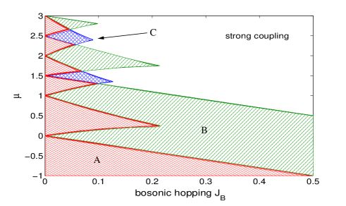
Figure 3: Color online) Phase diagram from strong-coupling expansion and $U=1,V=1.5$. Red areas (A) indicate truly incompressible Mott regions with gaped particle-hole excitations everywhere. Green (B) or blue (C) areas are partially compressible quasi-Mott regions with gaped particle-hole excitation for sites with (without) a fermion but ungapped excitation in the complementary region.

The system is truly incompressible only in the overlap region of the quasi-Mott lobes (A). Points which are within one of the two sequences of quasi-Mott lobes but not in both (cases B or C) are partially incompressible with an energy gap for a bosonic particle-hole excitation on a site with (B) (without (C)) a fermion but without a gap for a corresponding excitation on a complementary site. The properties of these partially incompressible phase will be discussed later.

These strong coupling results will now be complemented by numerical calculations using a DMRG simulation for a system with fixed fermion distribution an open boundary conditions. The local Hilbert space for the bosonic sector is $\text{span}\{|0\rangle,\dots,|6\rangle\}$, so it is truncated at $6$ bosons. The DMRG computation is done for both clustered and anti-clustered fermion distributions. The corresponding graphs for the phase boundaries are shown in Fig. 4.

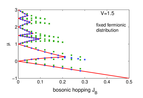
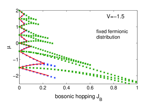
Figure 4: (Color online) Comparison of strong-coupling approximation (full line –) and DMRG for boundaries of incompressible phases for fixed distribution of fermions corresponding to clustering (inner crosses, $\boldsymbol{\times}$) or anti-clustering with maximum distance (outer crosses ,$\boldsymbol{\times}$) . $V=1.5$ (top figure) and $V=-1.5$ (bottom figure). $\rho_{F}=0.25$, and $U=1$.

One recognizes nearly perfect agreement between numerics and strong-coupling prediction in the case of clustering. This is expected since in the clustered case the majority of sites has neighbors of the same type. In the case of anti-clustering, however, the incompressible lobes extend much further into the region of large boson hopping with a critical $J_{B}$ of about 1 for a fermion filling of $\rho_{F}=1/4$ at $V=-1.5$. The latter is to be expected since in this case hopping to nearest neighbors is suppressed if the neighboring sites are of a different type ($\cal F$ or $\cal NF$). Here the curves of the critical chemical potential $\mu_{\rm crit}(J_{B})$ that correspond to a bosonic particle-hole excitation at a fermion site (here $\mu_{\rm crit}(0)=-1.5,-0.5,0.5,1.5$ etc.) start with a power $J_{B}^{\gamma}$ determined by the minimum number of hops required to reach the next fermion site, i.e. $\gamma=1/\varrho_{F}$, if $\rho_{F}\leq 1/2$. If the fermion filling is larger than $1/2$ the picture changes and the non-fermion sites (hole sites) cause $\mu_{\rm crit}(J_{B})\sim J_{B}^{\gamma}$ with $\gamma=1/(1-\rho_{F})$. In principle it is possible to extend the strong-coupling perturbation expansion to any fermion distribution, which is however involved. Fig. 5 shows the prediction of a cell-strong coupling expansion lit:Buonsante-PRA-2005 for an anti-clustered, fixed fermion distribution which is equivalent to bosons in a super-lattice potential .

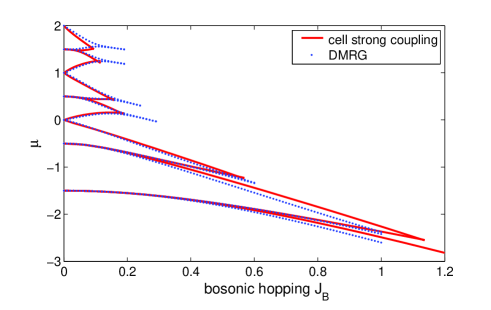
Figure 5: (Color online) Comparison of cell-strong coupling approximation (full line –) obtained from lit:Buonsante-PRA-2005 and DMRG for boundaries of incompressible phases for fixed distribution of fermions corresponding to anti-clustering with maximum distance (full dots,$\boldsymbol{\bullet}$) . $V=-1.5$, $\rho_{F}=0.25$, and $U=1$.

We now want to argue that the strong-coupling expansion for a clustered fermion distribution provides an accurate prediction for the boundaries of the incompressible phases in the case of quenched, random fermion disorder. Since in the thermodynamic limit any local distribution of fermions is realized at some places in the lattice, the actual phase boundaries are determined by the fermion configuration that leads to the smallest incompressible regions. Since this is the case for a clustered fermion configuration, which in turn is well described by the strong-coupling expansion, the latter gives a rather accurate description of the phase transition points between compressible and incompressible phases.

For the case of annealed fermion distribution the strong-coupling expansion is expected to give only less accurate results. This can be seen from Fig.6 where we compare the predictions of the strong-coupling approximation with those from a DMRG simulation for annealed fermionic disorder and a mean-field ansatz. Within the mean-field approach, e.g. of lit:Lewenstein-OptComm-2004 , hopping is included to the system as a perturbation to the ground state

$$\left|g\right.\rangle=\sqrt{1-\rho_{F}}\left|{n}_{0},0\right.\rangle+\sqrt{\rho_{F}}\left|{n}_{0}-s,1\right.\rangle.$$ (27)

Using this ground state and introducing a global bosonic order parameter $\psi$, the phase boundaries can be found using the usual Landau argumentation. For details see lit:Lewenstein-OptComm-2004 ; lit:Cramer-PRL-2004 . Fig.6 shows the resulting phase diagram compared to DMRG data for annealed disorder and strong-coupling predictions. When comparing the different data sets one recognizes that the mean-field predictions are qualitatively correct but as expected only moderately precise quantitatively. It should be mentioned that the accuracy of the mean-field approach becomes worse even for $J_{B}\to 0$ for a disorder with maximum anti-clustering. The numerical data were obtained by letting the DMRG code freely evolve in the manifold of fermionic distributions. The obtained distribution then gives a state which is at least close to the ground state. Since this procedure is prone to get stuck in local minima we checked the consistency of our results by implementing different sweep algorithms. In these algorithms the fermionic hopping was not taken to be zero but was given a finite initial value which was decreased during the DMRG sweeps to the final value zero. To ensure proper convergence we compared the data for a few representative points ($J_{B}=0.07$ boundaries of $(n_{0}=1,s=1)$ lobe; $J_{B}=0.15$ boundaries of $(n_{0}=1,s=0)$ lobe; $J_{B}=0.03$ boundaries of $(n_{0}=2,s=0)$ lobe) to the data obtained from two different sweep strategies . The difference in the chemical potential is of the order of $3\%$ independent of the sweep strategy an therefore negligible on the scale of the plot.

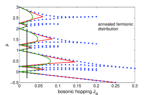
Figure 6: (Color online) Incompressible phases for an annealed fermion distribution and $U=1$, $V=0.25$, $\rho_{F}=0.25$. Shown are the strong-coupling results (outer full line –), the mean-field results from lit:Lewenstein-OptComm-2004 (inner full line –) and results from a DMRG calculation with $J_{F}=0$ (crosses $\boldsymbol{\times}$). Vertical line indicates position of the density cut shown in Fig.9 in the following section.

III.4 Influence of finite fermionic hopping

The question arises how the phase diagram changes if a finite but small fermionic hopping is included. The case $J_{F}\neq 0$ should be compared to the case $J_{F}=0$ for annealed fermionic disorder. Fig. 7 shows a comparison of DMRG data for $J_{F}=0$ and $J_{F}=J_{B}$. One recognizes that the influence of a small fermionic hopping is rather small.

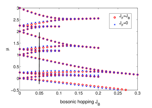
Figure 7: (Color online) Incompressible regions for $U=1$, $V=0.25$, $\rho_{F}=0.25$. Shown are the results from a DMRG calculation with $J_{F}=0$ and annealed fermionic disorder ($\boldsymbol{\times}$) and $J_{F}=J_{B}$ ($\circ$ ). The phases are the same as in fig. 6. Vertical line indicates position of the density cut shown in Fig.12.

III.5 Finite size extrapolation

The DMRG simulations are done for finite lattices and thus finite-size effects influence the results. To eliminate these effects each data point is obtained by a finite size extrapolation. This is particularly important if one wants to determine the critical values of $J_{B}$ for the compressible-incompressible transition. Figure 8 shows the extrapolation of the tip of the lowest Mott phase in Fig. 7 for $J_{F}=J_{B}$ to infinite lattice sizes $N\to\infty$. From a fit of $J_{c}$ to $\log(N)$ we find the critical point in the thermodynamic limit $J_{c}=0.16038$. The data for different system lengths show the expected $1/N$ behavior shown in Ref. lit:Kuehner-PRB-1998 for the BHM.

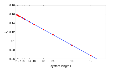
Figure 8: (Color online) Thermodynamic limit extrapolation for the critical point of the $n_{0}=1,s=1$ lobe ($\rho_{F}=1/4,\rho_{B}=3/4$) in figure 7. The critical point is found at $J_{c}=0.16038$

IV Partially incompressible phases

IV.1 Limit of vanishing fermionic hopping

Within the strong-coupling approximation discussed in the previous section we have identified regions in the $\mu-J_{B}$ phase diagram where bosonic particle-hole excitations are gapless if they occur on a fermion (non-fermion) site but have a finite gap on a complementary i.e. a non-fermion (fermion) site. Associated with this is a partial incompressibility

$$\frac{\partial\bigl{\langle}\sum_{i\in{\cal F}}{\hat{n}}_{i}\bigr{\rangle}}{\partial\mu}=0, \qquad\frac{\partial\bigl{\langle}{\sum_{i\in{\cal NF}}\hat{n}}_{i}\bigr{\rangle}}{\partial\mu}\neq 0,$$ (28)

or

$$\frac{\partial\bigl{\langle}\sum_{i\in{\cal NF}}{\hat{n}}_{i}\bigr{\rangle}}{\partial\mu}=0, \qquad\frac{\partial\bigl{\langle}\sum_{i\in{\cal F}}{\hat{n}}_{i}\bigr{\rangle}}{\partial\mu}\neq 0.$$

This is illustrated in Fig.9. Here the average boson number per site obtained from a DMRG simulation with annealed disorder is shown as a function of the chemical potential for constant bosonic hopping. The curve corresponds to the parameters of Fig.6 for the vertical cut shown in that figure at $J_{B}=0.02$. Also shown are the corresponding values only for fermion sites and non-fermion sites respectively. In the partially compressible phases the average boson number increases only for one type of sites while it stays constant for the other. In the DMRG code the energy per particle is calculated as a function of the total number of bosons $N$ which then yields the chemical potentials $\mu_{+}(N)=E(N+1)-E(N)$ and $\mu_{-}(N)=E(N)-E(N-1)$. Averaging over few values of $N$ in the compressible phase is needed here since the ground state fermion distribution changes with changing boson number leading to a non-monotonous dependence of $\mu$ on the boson number.

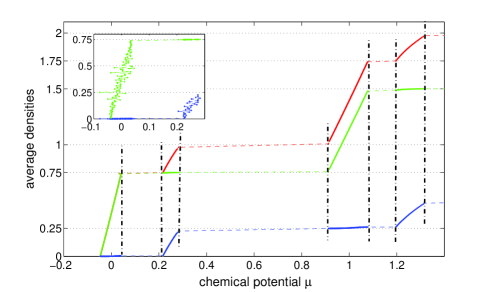
Figure 9: (Color online) Density cut along the vertical line in figure 6. From top to bottom: overall average density ( –), average density for sites without a fermion (–), average density for sites with a fermion (–). Inset: Dependence of particle number at one particular site as function of chemical potential without averaging.

We now discuss the properties of the single-particle density matrix $\langle{\hat{a}}_{i}^{\dagger}{\hat{a}}_{i+m}\rangle$ in the partially incompressible phases. For very large values of $J_{B}$ the system is expected to have a Luttinger-liquid behavior in 1d and to possess long-range off-diagonal order in higher dimensions. In 1d we expect that the Luttinger-liquid behavior disappears in the partially incompressible phases and that correlations decay exponentially. This is because in this case a single (static) impurity is sufficient to prevent the build-up of long-range correlations. In higher dimensions there will be a critical fermion (or hole) filling fraction above which off-diagonal order is suppressed. This critical fraction is determined by percolation thresholds and for annealed fermionic disorder depends on the actual fermion distribution in the ground state (e.g. clustered or anti-clustered). For a random fermion distribution in 2d the threshold is $\rho_{F}^{\rm crit}=0.5927$ (or $1-\rho_{F}^{\rm crit}=0.5927$ if non-fermion sites are incompressible). The corresponding number for 3d is $\rho_{F}^{crit}=0.3116$.

Fig.10 shows the first-order correlations $\langle{\hat{a}}_{i}^{\dagger}{\hat{a}}_{i+m}\rangle$ as function of the distance $m$ for an annealed fermion distribution obtained from DMRG simulations for a rather large lattice of 512 sites with incommensurate boson filling ($N_{B}=448$) and $\rho_{F}=1/4$. For $J_{B}=0.07$ strong exponential decay with correlation length $l_{c}=1.7$ is found corresponding to a glass-type behavior, while for $J_{B}=0.2$ correlations decay algebraically with $m^{-0.33}$, which corresponds to a Luttinger liquid. Note that for the chosen boson number, which corresponds to a non-commensurate value of $\hat{Q}$ there is no incompressible phase.

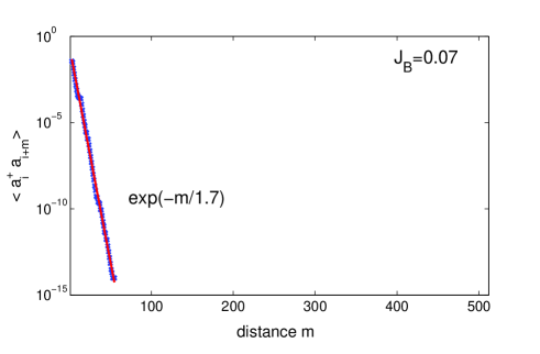
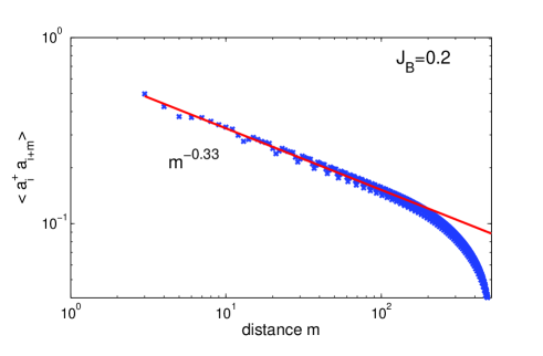
Figure 10: (Color online) DMRG simulations ($\boldsymbol{\times}$) of first-order correlations $\langle{\hat{a}}_{i}^{\dagger}{\hat{a}}_{i+m}\rangle$ for $V=0.25$, $\rho_{F}=0.25$ and $U=1$ for a lattice of 512 sites and $N_{B}=448$ bosons in the case of annealed disorder. (top curve:) $J_{B}=0.07$, line corresponds to exponential fit $\propto\exp\{-m/l_{c}\}$ with $l_{c}=1.7$. The exponential decay for small $J_{B}$ is apparent. (bottom curve:) $J_{B}=0.2$, line corresponds to algebraic fit $\propto m^{-\alpha}$ with exponent $\alpha=0.33$.

Fig. 11 shows the first-order correlations for a random, quenched fermion distribution averaged over 100 realizations with non-commensurate boson number ($\rho_{B}=N_{B}/N=184/128$). Despite the sampling noise one recognizes the transition between exponential decay with correlation length $l_{c}=2.9$ for $J_{B}=0.03$, and a power-law decay with $m^{-0.37}$ for $J_{B}=0.2$ corresponding to a Luttinger liquid. $J_{B}=0.03$ is within a partially incompressible phase, $J_{B}=0.2$ outside.

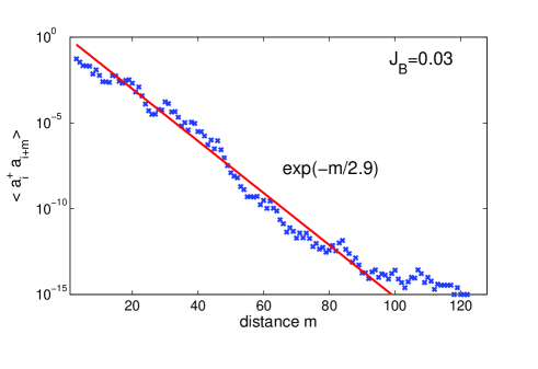
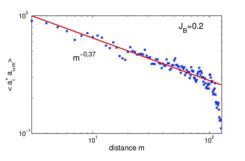
Figure 11: (Color online) DMRG simulations ($\boldsymbol{\times}$) of first-order correlations $\langle{\hat{a}}_{i}^{\dagger}{\hat{a}}_{i+m}\rangle$ for $V=1.5$, $\rho_{F}=0.375$ and $U=1$ for a lattice of 128 sites and $N_{B}=184$ bosons averaged over 100 fermion distributions. (top curve:) $J_{B}=0.03$, line corresponds to exponential fit $\propto\exp\{-m/l_{c}\}$ with $l_{c}=2.9$. The exponential decay for small $J_{B}$ is apparent. (bottom curve:) $J_{B}=0.2$, line corresponds to algebraic fit $\propto m^{-\alpha}$ with exponent $\alpha=0.37$. To avoid finite size effects at short and long ranges, only the sites in between $13$ and $110$ are taken into account.

The numerical results and the above discussion indicate that the partially incompressible phases have a glass-type character. A detailed discussion of the Bose-glass to superfluid transition will be given elsewhere lit:inprepBG .

IV.2 Small fermionic hopping

If there is a non-vanishing but small fermionic hopping, partial incompressibility is lost. Still the increase of the boson number with increasing chemical potential at one type of sites is substantially less that that on the complementary type of sites.

$$\frac{\partial\bigl{\langle}\sum_{i\in{\cal F}}{\hat{n}}_{i}\bigr{\rangle}}{\partial\mu} \ll \frac{\partial\bigl{\langle}{\sum_{i\in{\cal NF}}\hat{n}}_{i}\bigr{\rangle}}{\partial\mu}$$ (29)

or

$$\frac{\partial\bigl{\langle}\sum_{i\in{\cal NF}}{\hat{n}}_{i}\bigr{\rangle}}{\partial\mu} \ll \frac{\partial\bigl{\langle}\sum_{i\in{\cal F}}{\hat{n}}_{i}\bigr{\rangle}}{\partial\mu}.$$

Fig.12 shows the density cut obtained from DMRG simulations for the parameters of Fig.9 but for $J_{B}=J_{F}=0.05$. It should be noted that in contrast to Fig.9 averaging over sites is not needed due to the finite mobility of the fermions. The simulations show that the glass-type character of the phases survives. We expect a crossover from glass-type to Luttinger liquid behavior with increasing fermionic hopping. In addition due to the stronger back-action of the boson distribution to the fermion distribution other phases such as density waves emerge lit:Pazy-PRA-2005 . A discussion of the Bose-Fermi Hubbard model in the limit of large fermion mobility will be given elsewhere lit:Mering-2 .

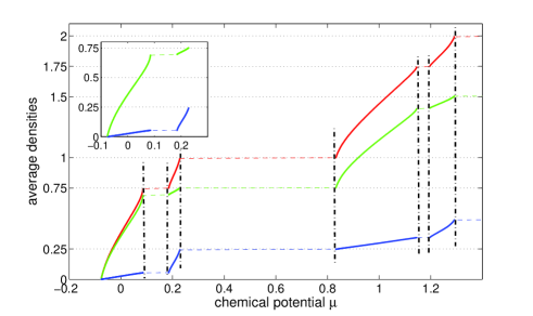
Figure 12: (Color online) Density cut for the same parameter as Fig.9 but for $J_{B}=J_{F}=0.05$ (see Fig.7).

V fluctuations

In this section, we will determine the fluctuations of the bosonic number operator for vanishing fermionic hopping $J_{F}=0$ inside the quasi Mott lobes for quenched disorder. To this end, second order perturbation theory will be applied and compared to numerical results from DMRG.

For vanishing bosonic hopping the ground state with a fixed number of fermions is clearly highly degenerate, from the distribution of $N_{F}$ fermions in a lattice with $N$ sites. For the case of quenched disorder with fixed positions of fermions, considered here, this degeneracy is inconsequential. This allows to develop a tractable approach based on non-degenerate perturbation theory for a given fermion distribution and subsequent averaging over all of these distributions. In order to evaluate the fluctuations of the bosonic number operator, we hence have to determine

$$\bar{n}={\mathbbm{E}}(\hat{n}_{j}),$$ (30)

which is independent of the lattice site $j$ due to translational invariance. Here, the classical average ${\mathbbm{E}}$ is taken with respect to the fermionic distributions, so the average over the $\binom{N}{N_{F}}$ different distributions with equal weight.

Figure 13: Possible single-hop excitations; the energies are given by $\Delta^{1}E$ to $\Delta^{4}E$ (see text for definitions). Filled circles are fermions, open circles bosons.

We can hence proceed as in Ref. lit:Plimak-PRA-2004 to compute the fluctuations in the boson number, for each fermion distribution, followed by the appropriate average. In second order perturbation theory in $J_{B}$ at $J_{F}=0$, only bosonic hoppings to nearest neighbors contribute. On such two sites, clearly, four different situations can arise, dependent on whether or not a fermion is present at each of the two sites, see Fig. 13. The change in energy due to these excitations is given by (here, we have no longer taken $U=1$)

$$\Delta^{(1)}E = \Delta^{(4)}E=-U,$$ (31)

$$\Delta^{(2)}E = -U(1-s)-V,$$ (32)

$$\Delta^{(3)}E = -U(1+s)+V,$$ (33)

where the superscript denotes the type of process according to Fig. 13. With this we are now able to calculate the fluctuations ${\mathbbm{E}}\langle\Delta\hat{n}^{2}_{j}\rangle$ of the bosonic number operator. After a number of steps, following the procedure of Ref. lit:Plimak-PRA-2004 , we find

$${\mathbbm{E}}\langle\Delta\hat{n}^{2}_{j}\rangle = 2z\left(\frac{J_{B}}{U}\right)^{2}{n}_{0}({n}_{0}+1)(1-\rho_{F})^{2}$$ (34)

$$+ 2z\left(\frac{J_{B}}{U}\right)^{2}({n}_{0}-s)({n}_{0}-s+1)\rho_{F}^{2}$$

$$+ 2zJ_{B}^{2}\frac{{n}_{0}({n}_{0}-s+1)+({n}_{0}-s)({n}_{0}+1)}{U^{2}-(Us-V)^{2}}$$

$$\times \rho_{F}(1-\rho_{F}),$$

where $z$ gives the number of nearest neighbors. The fluctuations show the expected quadratic dependence on the hopping strength. Moreover, in the two limiting cases $\rho_{F}=0$ and $\rho_{F}=1$ this expression coincides with the pure BHM result from Ref. lit:Plimak-PRA-2004 . Fig. 14 shows the analytical result compared with DMRG calculations for annealed disorder. For small $J_{B}$ the agreement is rather good with increasing disagreement for bigger $J_{B}$, where second order perturbation theory starts to fail.

Fig. 15 shows the dependence of the fluctuations of the fermionic density $\varrho_{F}$ at a fixed hopping $J_{B}$. Also shown is one numerical curve obtained with annealed disorder. The agreement between the analytical expression (34) and the numerical data shows, that the above derivation gives a good estimate for the fluctuations in the system for small bosonic hopping.

Figure 14: (Color online) Bosonic number fluctuations in the Mott-insulating lobes for different lobes at fixed density for annealed disorder. The upper three lines are for $V=1.25$, $\rho_{F}=0.375$, $s=1$ with ${n}_{0}=1$($\blacktriangleright$), $2$($\blacktriangleright$) and $3$($\blacktriangleright$) scaled by $10^{3}$. Lower three lines: $V=1.7$, $\rho_{F}=7/16$, $s=2$ with ${n}_{0}=2$($\bullet$), $3$($\bullet$) and $4$($\bullet$); solid lines are the corresponding analytic curves

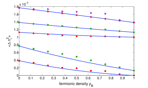
Figure 15: (Color online) Bosonic number fluctuations in the quasi Mott lobes for different lobes at fixed hopping. The upper three lines are the results for $V=1.25$, $J_{B}=0.004$, $s=1$ with ${n}_{0}=1$ ($\blacktriangleright$), $2$ ($\blacktriangleright$) and $3$ ($\blacktriangleright$), shifted by $10^{-3}$ upwards; lower two lines: $V=1.7$, $J_{B}=0.004$, $s=2$ with ${n}_{0}=2$ ($\bullet$) and $3$ ($\bullet$); solid lines are the corresponding analytic curves. Red circles ( $\circ$) are the corresponding fluctuations for a clustered disorder (only for the uppermost plot).

VI Summary

In the present paper we have analyzed the $\mu-J_{B}$ phase diagram of the one-dimensional semi-canonical Bose-Fermi Hubbard model with fixed number of fermions in the limit of vanishing fermion mobility, i.e. $J_{F}\to 0$. This limit is equivalent to a Bose-Hubbard model with a random modulation of the one-site energy. An important difference to the disordered Bose-Hubbard model lit:Fisher-PRB-1988 lies however in the distribution of on-site energies which is here not continuous but binary, corresponding to the presence or absence of a fermion at a given site. As a consequence there are no extended compressible phases for vanishing bosonic hopping. Instead incompressible phases with in general incommensurate boson number emerge similar to the case of a super-lattice lit:Roth-PRA-2003 ; lit:Buonsante-PRA-2004 . These Mott-insulating phases which can be characterized by two integer parameter $n_{0}$ and $s$, denoting the number of bosons at sites without a fermion and the shift of this number due to the presence of a fermion have been predicted before within mean-field and Gutzwiller approaches lit:Lewenstein-PRL-2004 ; lit:Cramer-PRL-2004 . Here we determined the extend of these phases using a modified strong-coupling expansion and numerical simulations employing the density-matrix renormalization group (DMRG). We showed that the shape of the quasi-Mott lobes depends on the actual fermion distribution. The latter is determined by the preparation technique. If the fermionic hopping is small but sufficiently large such that the fermions have time to find the energetically lowest configuration, one has an annealed fermionic disorder, otherwise the distribution is random and frozen. For the annealed case we showed that in the limit of small, but nonzero bosonic hopping, $J_{B}$, the fermions form either a clustered or an anti-clustered configuration with maximum mutual distance. A partial explanation for this behavior could be found in terms of the composite-fermion model of lit:Lewenstein-PRL-2004 . For the case of random, quenched fermion distributions we could derive semi-analytic predictions for the phase boundaries of the incompressible phase using a strong-coupling approach lit:Freericks-PRB-1996 which agreed very well with numerical simulations. Within this approach we also identified partially compressible phases where particle-hole excitations at one type of site, i.e. either with or without a fermion, are gap-less, while the corresponding excitations at the complementary type of sites are gapped. The partial compressibility of these phases was verified by numerical simulations. We also showed that that the presence of partial compressibility lead to Bose-glass phases, which are gap-less but for which first-order correlations decay exponentially. We discussed the influence of a finite bosonic hopping on local properties in the quasi-Mott phases using a perturbative approach supplemented by numerical DMRG simulations. Finally we also discussed the influence of a finite fermionic hopping. The numerical simulations indicate that many predictions remain valid for finite values of $J_{F}$ even as large as $J_{B}$. A more detailed discussion of the limit of large fermionic hopping and the associated new phenomena such as density waves etc. will be given elsewhere lit:Mering-2 .

VII Acknowledgements*

We would like to thank M. Cramer, J. Eisert, L. Plimak, U. Schollwöck, and M. Wilkens for stimulating discussions. We are also indebted to U. Schollwöck for providing the DMRG code and his support in numerical questions. Finally we would like to thank P. Buonsante and A. Vezzani for providing the cell-strong coupling data for Fig.5. This work has been supported by the DFG (SPP 1116, GRK 792) and NIC at FZ Jülich.

References

- (1) I. Bloch, J. Dalibard, and W. Zwerger, arXiv:0704.3011v1.
- (2) D. Jaksch and P. Zoller, Annals of Physics, 315, 52 (2005). cond-mat/0410614v1.
- (3) M. Greiner, O. Mandel, T. Esslinger, T.W. Hänsch, and I. Bloch, Nature 415, 39 (2002).
- (4) M. P. A. Fisher, P. B. Weichman, G. Grinstein, and D. Fisher, Phys. Rev. B 40, 546 (1988).
- (5) D. Jaksch, C. Bruder, J. I. Cirac, C. W. Gardiner, and P. Zoller, Phys. Rev. Lett., 81, 3108 (1998).
- (6) P. Lugan, D. Clement, P. Bouyer, A. Aspect, M. Lewenstein, and L. Sanchez-Palencia, Phys. Rev. Lett. 98, 170403 (2007).
- (7) M. Lewenstein, A. Sanpera, V. Ahufinger, B. Damski, A. Sen De, and U. Sen, cond-mat/0606771.
- (8) S. Rapsch, U. Schollwöck, and W. Zwerger, Europhys. Lett. 46, 559 (1999).
- (9) F. Ferlaino, E. de Mirandes, G. Roati, G. Modugno, and M. Inguscio, Phys. Rev. Lett. 92, 140405 (2004).
- (10) K. Günter, T. Stöferle, H. Moritz, M. Köhl, and T. Esslinger, Phys. Rev. Lett. 96, 180402 (2006).
- (11) C. Ospelkaus, S. Ospelkaus, K. Sengstock, and K. Bongs, Phys. Rev. Lett. 96, 020401 (2006).
- (12) Z. Hadzibabic, C. A. Stan, K. Dieckmann, S. Gupta, M.W. Zwierlein, A. Göerlitz, and W. Ketterle, Phys. Rev. Lett. 88, 160401 (2002).
- (13) A. Albus, F. Illuminati, and J. Eisert, Phys. Rev. A 68, 023606 (2003).
- (14) M. Lewenstein, L. Santos, M. A. Baranov, and H. Fehrmann, Phys. Rev. Lett. 92, 050401 (2004).
- (15) H. Fehrmann, M. A. Baranov, B. Damski, M. Lewenstein, and L. Santos, Opt. Comm. 243, 23 (2004).
- (16) M. Cramer, J. Eisert, and F. Illuminati, Phys. Rev. Lett. 93, 190405 (2004).
- (17) R. Roth and K. Burnett, Phys. Rev. A 69, 021601(R) (2004).
- (18) E. Pazy and A. Vardi, Phys. Rev. A, 72, 033609 (2005).
- (19) L. Mathey, D.-W. Wang, W. Hofstetter, M. D. Lukin and E. Demler, Phys. Rev. Lett. 93, 120404 (2004).
- (20) A. Imambekov and E. Demler, Phys. Rev. A, 73, 021602 (2006).
- (21) H. P. Büchler and G. Blatter, Phys. Rev. Lett 91, 130404 (2003).
- (22) H. P. Büchler and G. Blatter, Phys. Rev. A 69, 063603 (2004).
- (23) L. Pollet, et al., Phys. Rev. Lett. 96, 190402 (2006.
- (24) L. Pollet, C. Kollath, U. Schollwöck, and M. Troyer, cond-mat/0609604.
- (25) J. K. Freericks and H. Monien, Phys. Rev. B 53, 2691 (1996).
- (26) T. D. Kühner and H. Monien, Phys. Rev. B 58, 14741 (1998).
- (27) U. Schollwöck, Rev. Mod. Phys. 77, 000259 (2005).
- (28) R. Roth, and K. Burnett, Phys. Rev. A, 68, 023604 (2003).
- (29) P. Buonsante and A. Vezzani, Phys. Rev. A 70, 061603(R) (2004).
- (30) P. Buonsante and A. Vezzani, Phys. Rev. A 72, 013614 (2005).
- (31) L. D. Landau and E. M. Lifschitz, Quantum mechanics (Akademie-Verlag, Berlin).
- (32) D. C. Roberts and K. Burnett, Phys. Rev. Lett. 90, 150401 (2003).
- (33) A. Mering, M. Fleischhauer, M. Cramer, J. Eisert and U. Schollwöck, (in preparation)
- (34) L. I. Plimak, M. K. Olsen, and M. Fleischhauer, Phys. Rev. A 70, 013611 (2004).
- (35) A. Mering and M. Fleischhauer, (to be published).