On the Search for Quasar Light Echoes

Abstract

The UV radiation from a quasar leaves a characteristic pattern in the distribution of ionized hydrogen throughout the surrounding space. This pattern or light echo propagates through the intergalactic medium at the speed of light, and can be observed by its imprint on the Ly$\alpha$ forest spectra of background sources. As the echo persists after the quasar has switched off, it offers the possibility of searching for dead quasars, and constraining their luminosities and lifetimes. We outline a technique to search for and characterize these light echoes. To test the method, we create artificial Ly$\alpha$ forest spectra from cosmological simulations at $z=3$, apply light echoes and search for them. We show how the simulations can also be used to quantify the significance level of any detection. We find that light echoes from the brightest quasars could be found in observational data. With absorption line spectra of 100 redshift $z\sim 3-3.5$ quasars or galaxies in a 1 square degree area, we expect that $\sim 10$ echoes from quasars with B band luminosities $L_{B}=3\times 10^{45}$ ergs^-1 exist that could be found at 95 % confidence, assuming a quasar lifetime of $\sim 10^{7}$ yr. Even a null result from such a search would have interesting implications for our understanding of quasar luminosities and lifetimes.

1. Introduction

The Ly$\alpha$ forest in quasar spectra (see e.g. Rauch 1998 for a review) offers a useful means to probe the density and ionization structure of the high redshift intergalactic medium. The predictions of cosmological simulations (Cen et al. 1994; Zhang, Anninos, & Norman 1995; Petitjean, Mücket, & Kates 1995; Hernquist et al. 1996; Katz et al. 1996; Wadsley & Bond 1997; Theuns et al. 1998; Davé et al. 1999) have been seen to match observational data well (e.g., Viel et al. 2004). In current cosmological theories, the Ly$\alpha$ forest is produced by the remnant neutral hydrogen in a smoothly fluctuating density field of largely photoionized gas. The fluctuations in the Ly$\alpha$ optical depth $\tau$ are predicted (see e.g., Weinberg et al. 1997, Croft et al. 1997) to be related to the gas density ($\rho$) at each point (${\bf x}$) and inversely proportional to the intensity $J$ of the ionizing background radiation field:

$$\tau\propto\rho({\bf x})^{\sim 1.6}/{J({\bf x})}$$ (1)

Close to the brightest sources, quasars, the effect of increased $J$ is strong enough that it has been possible to detect the decrease in Ly$\alpha$ forest absorption along the same quasar sightline, the so-called proximity effect (Bajtlik et al. 1988, Scott et al. 2000). Quasar radiation is expected to travel not only along the line of sight, but also transverse to it, and affect the ionization state of the IGM which can be probed by adjacent sightlines. This effect, known as the transverse, or foreground proximity effect has not yet been seen convincingly in hydrogen Ly$\alpha$ forest data (e.g., Schirber et al. 2004, Croft 2004, although see Dobrzycki & Bechtold 1991).

In general, the presence of discrete sources of photoionizing radiation will lead to spatial fluctuations in $J({\bf x})$. The statistical properties of these have been explored by many authors, including for example Zuo (1992) and Meiksin & White (2003). Strong sources such as quasars will leave particularly recognizable imprints in the intergalactic radiation field (see Figure 5 of Croft 2004). Their size, shape and strength can be probed using multiple Ly$\alpha$ spectrum sightlines, in a generalization of the transverse proximity effect. Adelberger (2004) has shown how sightlines chosen around observed quasars can be used to measure the radiative histories of quasars through the transverse proximity effect. We choose to use the term “light echo” to describe these features because although they are not directly analogous to supernova light echoes (e.g., Crotts et al. 1989) the light from quasars is still detectable through them after the quasars themselves have become “quiet”. We will explain in §2 how we can find the light echoes and so detect quasars and yield constraints on their properties even when the light from them is not directly observable.

There are several examples of extended objects which have been searched for in cosmological datasets with some type of matched filtering. These include galaxy clusters at high redshift (Postman et al. 1996). Circles in the CMB sky, which would be a sign of a universe with a small topology scale have also been looked for (Cornish et al. 2004). We will use a similar idea to find and measure light echoes in Ly$\alpha$ forest data, searching for the signature of a deficit of Ly$\alpha$ absorption with a particular geometry.

The lifetimes of quasars are relatively poorly constrained, and observationally the evidence points to the range $10^{6}-10^{8}$ Yr (see Martini 2003 for a review). Theoretical predictions of quasar lifetimes have recently become available from hydrodynamic simulations of galaxy formation which include black hole accretion and feedback (e.g., Di Matteo et al. 2005, Hopkins et al. 2005). Successfully measuring the transverse proximity effect or finding a light echo would represent one way to test these models.

This paper is structured as follows. In §2 quasar light echoes are outlined in more detail. In §3 the simulations used to produce spectra to which light echoes were artificially applied are described. In §4 a technique is described to search for quasar light echoes in Ly$\alpha$ spectra. In §5 the results of searches for light echoes in simulated data are presented. These results include the sensitivity of the test to different quasar luminosities and to varying the number of and resolution of Ly$\alpha$ spectra. In §6, we discuss our results, computing the chances of finding a light echo in observational data and the volume of data that would be required to do so.

2. Quasar Light Echoes

The radiation emitted from a quasar has an effect on the ionization state of the gas through which it passes. If a quasar produced high levels of radiation for some period of time a signature will be left in the surrounding gas long after this period has stopped. There will be lower levels of neutral hydrogen in the region affected by the propagating radiation from the once active quasar, as described by Equation 1. The equilibration time, the time taken for the ionization state to respond to small changes (factors of a few) in the intensity of the ionizing radiation is of the order of $10^{4}$ yr (Martini 2003). As this is much shorter than the quasar lifetimes we will be considering, the effect of the quasar radiation will effectively propagate through the intergalactic medium at the speed of light. The width of the light echo will be equal to the light travel time multiplied by the length of time the quasar was radiating.

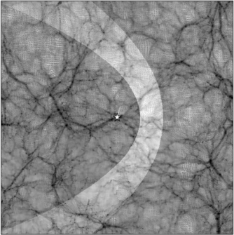
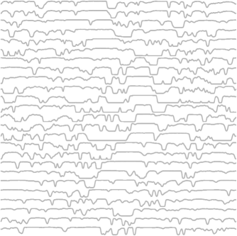
Figure 1.— Top panel: The neutral hydrogen density in a $1\;h^{-1}{\rm Mpc}$ thick slice through a simulation of a $\Lambda$CDM universe. The plot width is $50$ comoving $\;h^{-1}{\rm Mpc}$. A quasar light echo has been applied and can be seen, the quasar (position shown by a star symbol) having a lifetime $t_{q}=8.2$ My and switching off 8.2 My ago. The observer is observing from the left side of the plot, the line-of-sight being the $x-$axis Bottom panel: 25 Ly$\alpha$ spectra have been made in the plane of the top figure, showing the effect of the quasar light echo. This arrangement of spectra is a very artificial situation, but illustrates how a light echo can be seen. The high flux regions in the spectra correspond to areas of low neutral hydrogen density caused by the light echo.

For simplicity, in the present paper we approximate the quasar lightcurves by a top hat i.e., we assume that a quasar starts to emit a constant level of radiation and stops sharply some time $t_{q}$ later. We will also assume that this takes place at a redshift where the expansion timescale is significantly less than $t_{q}$, so that we can model the quasar radiation using the inverse square law. An additional simplification we use is to neglect the attenuation of the quasar due to intergalactic absorption. As the attenuation length at $z=3$ is of the order of $100\;h^{-1}{\rm Mpc}$ (Haardt & Madau 1996) this is not a bad approximation.

If we were able to recieve information from all points in space at the same time, a light echo would be a spherical shell. The outer boundary would correspond to the start of emission and the inner one correspond to the end, with a separation $ct_{q}$ between them. However, when observing a light echo one would not be able to see every point in space at the same time. The boundaries of the regions containing radiation can be described as follows. Given a Cartesian coordinate system with the $z-$axis being oriented directly away from the observer and the origin centered on the quasar:

$$R_{on}=ct_{on}-z,$$ (2)

where $R_{on}$ is the distance the light has traveled since the start of radiation emission and $t_{on}$ is the time since the start of this emission considered at the location of the quasar.

Changing to spherical coordinates one obtains

$$R_{on}=ct_{on}-R_{on}\cos(\theta)$$ (3)

Thus, the surface corresponding to the start of the radiation can be described as

$$R_{on}=\frac{ct_{on}}{1+\cos(\theta)}$$ (4)

Another surface can be constructed in exactly the same way using, $t_{\rm off}$, the time since the quasar emission has stopped considered at the location of the quasar. The light echo is then the region enclosed by the two surfaces $R_{on}$ and $R_{\rm off}$.

There are six parameters which describe the precise shape of the quasar light echo: the length of time since the quasar started and stopped emitting radiation, the three dimensional coordinates of the quasar and the luminosity of the quasar.

In the top panel of Figure 1, we show an example of a light echo from a bright quasar applied to a slice from a cosmological simulation (described in §3). The neutral hydrogen density is shown as shades of gray, and the shape of the light echo can be seen clearly.

In the examples in this paper, we assume that the quasar radiates its energy isotropically. Unified models of Active Galactic Nuclei (e.g., Urry & Padovani 1995), however predict that the ionizing radiation may be beamed into a cone with opening angle $\sim 90\deg$ (a solid angle of $\sim 1.8$ rad.) This cone would restrict the geometry of the light echo. In this case, the signal to noise ratio of a light echo detection would be reduced by approximately $\sim\sqrt{(}1.8/4\pi)\sim 0.4$ unless extra parameters were introduced to model the beaming. We leave investigation of this possibility to future work (see also Croft 2004, Adelberger 2004.)

3. Simulations

We use cosmological N-body simulations of a $\Lambda$CDM universe in order to develop and test our light echo search technique. The cosmological parameters we assume are consistent with the first year WMAP results (Spergel et al. 2003) and are Hubble constant $H_{0}=70{\rm\;km\;s^{-1}}{\rm Mpc}^{-1}$, $\Omega_{M}=0.3$, $\Omega_{\Lambda}=0.7$, amplitude of mass fluctuations, $\sigma_{8}=0.9$. Our simulations are dark matter only, run with the N-body code Gadget (Springel, Yoshida & White 2001) in a periodic cubical volume of side length $50\;h^{-1}{\rm Mpc}$, ($h=H_{0}/100{\rm\;km\;s^{-1}}{\rm Mpc}^{-1}$) with $256^{3}$ particles. We carry out 20 runs with different random phases, and use output snapshots at redshift $z=3$.

We make Ly$\alpha$ spectra from the simulations by assigning an SPH-like smoothing kernel to each dark matter particle to mimic the distribution of gas in the IGM. We then integrate along sightlines through the kernels in the usual manner (e.g., Hernquist et al. 1996), computing the density in pixels. We use the Fluctuating Gunn-Peterson Approximation (e.g., Weinberg et al. 1997) to assign a Ly$\alpha$ optical depth to each pixel, and a power-law temperature density relation $T=T_{0}(\rho/\overline{\rho})^{0.6}$ to assign temperature. Here $T_{0}=$20000 K (see e.g., Schaye et al. 2000) and $\overline{\rho}$ is the mean density of baryons in the Universe. We note that the adiabatic index is likely to be lower than $0.6$ at $z=3$ (observations such as Schaye et al. 2000 suggest an isothermal equation of state.) The large scale fluctuations in the Ly$\alpha$ forest are however insensitive to this choice (see e.g., Fig. 7 of Croft et al. 1998.) We convolve the real space distribution of optical depths with the thermal broadening and the line-of-sight peculiar velocity field to produce spectra in observable units (in redshift space).

In carrying out this procedure, we first assume a uniform ionizing radiation field throughout the volume. We normalize the $\tau$ values so that the value of the mean transmitted flux $\langle F\rangle=0.696$, that observed by Schaye et al. (2003). We also make spectra with light echoes. In this case, we choose the position of the quasar (in this paper, we pick random locations) and apply the light echo to the real space optical depths in the spectra using Equations 1-4. After the light echo has been applied we convolve the spectra with thermal broadening and peculiar velocities.

In the bottom panel of Figure 1 we show an example of 25 spectra that correspond to the neutral hydrogen density field in the simulation slice above it. In this case, the sightlines were taken to all lie in a plane. This is an obviously artificial situation for illustrative purposes only, and in the rest of the paper we assume that the sightlines are randomly distributed. We can see the outline of the light echo in the Ly$\alpha$ forest of Figure 1, but it is difficult to distinguish by eye. We shall see below that by passing a template through the datasets we can detect the light echoes and compute their significance level.

Using the spectra in the simulations, we construct fiducial artificial datasets, all at redshift $z=3$. Our fiducial datasets contain 50 spectra each and we rebin the high resolution pixels to 50 pixels per spectrum, corresponding to a pixel size of 1.8 Angstroms. In order to determine the statistical significance of light echo detections, as detailed in our method below, it is necessary to create 1000 artificial datasets. We do this by computing 50 sets of spectra (always with the same positions, initially randomly chosen), for each of the 20 simulations with random phases, but for each set randomly translating the box, rotating it through a multiple of 90 degrees about the 3 axes and randomly reflecting it.

4. Search Technique

To search for a quasar light echo in a set of spectra, we create templates by applying a light echo artificially to uniform spectra (all pixels initially have transmitted flux $F=\langle F\rangle$ with the same spatial configurations.) The data being searched is then compared to the templates. A value of $\chi^{2}$ is then computed by comparing pixels in the template with those in the dataset:

$$\chi_{{\rm pre-norm}}^{2}=\displaystyle\sum_{i=1}^{N}\displaystyle\sum_{j=1}^{M}\left(\frac{F_{\rm temp}-F_{\rm data}}{\sigma}\right)^{2}$$ (5)

Here $N$ is the number of spectra, $M$ is the number of pixels per spectrum, $F_{\rm temp}=e^{-\tau_{\rm temp}}$, and $F_{\rm data}=e^{-\tau_{\rm data}}$, are the transmitted flux in pixels for the template and the data respectively. The standard deviation of the pixel values $F_{\rm data}$ in the data is used to compute $\sigma$. Our estimate of the “noise” will therefore be dominated by the intrinsic density fluctuations in the transmitted flux. We do not however compute the full covariance matrix, but instead will compute the significance of light echo detections by looking at the probablity of false detections in simulated datasets with no light echoes (see below).

Figure 2.— A search for a light echo in one dimension. We plot the $\chi^{2}$ that results when fitting light echo templates with a varying $z$ coordinate for the quasar position (distance from the boundary of the simulation box along along the line of sight to the observer). We fit the templates to a simulated observational dataset with an imposed light echo (true quasar position is $z=25\;h^{-1}{\rm Mpc}$). The top panel shows the results (as circles) before subtracting the background average $\chi^{2}$ (this background is also shown as filled squares) while the bottom panel shows the renormalized results (see §4 for details).

When we compute the $\chi^{2}$ value in Equation 5, we make sure to compute the standard deviation $\sigma$ for each data set separately. Without doing this, we find that the significance of detections is degraded by an order of magnitude or more.

In our technique, a grid of values for each parameter describing a light echo is set up and a template is made for each possible combination of these values. If a template has a very low $\chi^{2}$ it is likely that there is a quasar light echo in the data with the same parameters as the template.

The less space an echo occupies in the template (for example if the echo is on the far edge of the simulation box closest to the observer), the lower the $\chi^{2}$ values tend to be. To account for this it is necessary to renormalize the likelihoods. To do this, we find the $\chi^{2}$ values of all the templates fitted to many mock spectra generated without applied light echoes and average them. This average $\chi^{2}$ is then subtracted from the pre-normalized $\chi^{2}$ values determined as described above giving:

$$\chi^{2}=\chi_{\rm pre-norm}^{2}-\chi_{\rm avg}^{2}$$ (6)

By doing this we are subtracting the distribution of $\chi^{2}$ values which arises purely from the geometry of the sample, to reveal the true light echo signal. After doing this, we identify the templates with the lowest $\chi^{2}$ values. Because we have only applied one light echo to the simulated data and are searching for that, we associate the minimum $\chi^{2}$ value with the echo we are searching for. In a real observational dataset, our search could include the possibility of multiple minima in the $\chi^{2}$, corresponding to the presence of several light echoes.

After the lowest $\chi^{2}$ is found, we determine the statistical significance of the detection. We do this by applying the same search procedure to our 1000 simulated datasets, but without having applied light echoes to them. The statistical significance is the probability that an equal or lower $\chi^{2}$ could be caused by statistical fluctuations. These statistical fluctuations correspond to density fluctuations which by chance mimic the geometry of a light echo. These could occur anywhere in the simulation volume.

In summary the light echo search technique consists of the following steps:
1. Pick a range of values and create a grid of the six parameters ($x,y,z,t_{\rm off},t_{\rm on},L$) describing a light echo.
2. Create a template for every point on this grid and compare with data to calculate $\chi^{2}$ for each.
3. Subtract average $\chi^{2}$ computed from many simulated spectra without light echoes to obtain normalized $\chi^{2}$
4. Find $\chi^{2}$ minimum.
5. Create many simulated spectra with the same coordinates, but without a light echo.
6. Repeat steps 3-5 on each set of simulated spectra and count fraction of cases with lower $\chi^{2}$ to determine statistical significance.

5. Tests and results

Figure 3.— Statistical significances for detection of light echoes in mock observational data (see §5) as a function of quasar luminosity. The four different curves correpond to four different simulated datasets with different random seeds. In the top panel the light echoes being searched for all had a lifetime $t_{q}=16.3$ Myr and a time since the end of radiation emission of 16.3 Myr (see text: case A.) Different sets of mock observational data were made with different quasar blue band luminosities and the statistical significance of detection is plotted versus that luminosity. In the bottom panel (text: case B) the light echoes in the mock data all had lifetime $t_{q}=32.6$ Myr and time since the end of emission 65.2 Myr (i.e. the light echo was much farther from the position of the quasar than in the top panel).

We set up a test light echo inside the cubical volume of the simulation and use our search technique described above to find and parametrize it. The location of the quasar was chosen to be in the center of the box. The duration of time since the beginning and end of the radiation emission were set to be 32.6 Myr and 16.3 Myr respectively ($t_{\rm on}$ and $t_{\rm off}$ in Eqns. 2-4). The quasar lifetime ($t_{\rm on}-t_{\rm off}$) in this case was therefore 16.3 Myr. We refer to this as test case A.

In order to make our testing more widely applicable, an additional, different test (case B) was also set up, this time with the echo located much further from the quasar position (i.e. the time since the quasar switched off is much longer). This time the quasar is located at $x,y$ and $z$ coordinates of $(25,25,10)\;h^{-1}{\rm Mpc}$, where the $z-axis$ is oriented along the line of sight towards the observer. The $t_{\rm on}$ and $t_{\rm off}$ times were 97.8 Myr and 65.2 Myr respectively, so that the quasar lifetime is 32.6 Myr, double that of the previous case.

Figure 4.— Statistical significances of finding a quasar light echo with a blue-band luminosity of $2\times 10^{45}$ erg/s with differing number of spectra in the mock observational dataset. All spectra had 50 pixels each (1.8 Åwidth). Four simulations with different random seeds were used to make the 4 different lines.

For each of these two test cases, we create a simulated dataset, using a number of spectra which could be achievable with observations (see §6.2 for further discussion). As stated in §3, We pick 50 spectra passing through the simulation volume, which subtends an angle on the sky of 39 arcmin at $z=3$. We note that we only use a fraction of the information available in each spectrum as each full Ly$\alpha$ to Ly$\beta$ region is 7 times the length of our simulation box. In §5.2 below we will investigate the effect of varying pixel size and number of quasar spectra on the ease of detection of light echoes.

We used our 1000 sets of simulated spectra to find the average background likelihood distribution as well to calculate the statistical significance of located echoes. In the tests, we set up a grid of search parameters, with a $5\;h^{-1}{\rm Mpc}$ spacing in the $x,y,z$ coordinates of the quasar, and also a 8.2 Myr spacing in $t_{\rm on}$. In the present work, we have chosen to not search through the other parameters ($t_{\rm off},L$) at the same time, but instead assume that they are known. We then vary them individually in later tests to show that they can be constrained. We leave it to future work to search through the 6 dimensional grid directly.

In order to deal with the effect of not varying $t_{\rm off}$, we assume that a template used to search for light echoes would be discretized so that $t_{\rm off}-t_{\rm on}=\Delta t,$ where $\Delta t$ is an interval of time equal to the shortest quasar lifetime to be searched for. In this way only one of the two parameters $t_{\rm off},t_{\rm on}$ needs to be searched for directly and if the actual quasar lifetime $t_{q}$ is greater than $\Delta t$ then multiple light echoes will be detected originating in the same place but at different times. They can be summed together to recover the full echo.

In Figure 2 is an example plot showing how the $\chi^{2}$ varies as a function of coordinate $z$ , distance along the line of sight to the observer, for all other parameters held fixed at the input values used to construct the light echo. The panels show the raw $\chi^{2}$ and the renormalized $\chi^{2}$, obtained after subtracting the background average from all the random realizations. We can see that the minimum in the $\chi^{2}$ is at the input value, for this, test case A, $z=25\;h^{-1}{\rm Mpc}$.

5.1. Sensitivity of Technique to Light Echoes of Different Luminosities

The effect of the light echoes on the Ly$\alpha$ forest depends on the ratio of the quasar radiation intensity to the UV background intensity. The background in our test cases was set to be $5\times 10^{-22}\frac{erg}{(s)(Hz)(Sr)(cm^{2})}$, consistent with the results of Rauch et al. (1997).

The restframe blue-band luminosity of each quasar was calculated by approximating the luminosity per frequency interval as being $\propto\nu^{-1}$ and integrating over the rest frame Blue-band.

$$L=\int\frac{A}{\nu}d\nu$$ (7)

The spectral radiance of ionizing radiation is then compared to that of the backround radiation:

$$E_{\nu}=\frac{A\cdot 91.2nm}{c\cdot 4\pi(sr)(r/[1+z])^{2}}$$ (8)

where $A$ is the constant from the luminosity equation above and $r$ is the comoving distance from the quasar.

Quasar light echoes corresponding to quasars of different blue-band luminosities were applied to identical sets of spectra and then used to determine the sensitivity of the search technique. In order to gauge how the significance can vary from quasar to quasar we chose 4 different simulations with different random seeds to make our simulated datasets and show results for each of these test cases separately in the plots.

Figure 3 shows the statistical significance of each detected quasar light echo, i.e. the fraction of simulation datasets with no light echo that gave a lower $\chi^{2}$ somewhere in the parameter space.

The blue-band luminosity required to detect a light echo, in case A, at better than $0.1\%$ statistical significance (i.e. $>99.9\%$ confidence level of detection) for the particular shape of echo used is between $3.5-5\times 10^{45}$ erg/s. Taking the upper end of this range, this corresponds to an AB magnitude M${}_{\rm B}\simeq-25.4$ being needed for detection. For $95\%$ confidence, we need $\sim 3\times 10^{45}$ erg/s, or M${}_{\rm B}\simeq-24.8$.

Additionally we tested case B, the light echo which has a much longer time since the quasar switched off. In this case, the echo is fainter and the B-band luminosity required for $95\%$ confidence is $5\times 10^{45}$ erg/s. For $99.9\%$ confidence the luminosity in this case was $\sim 10-15\times 10^{45}$ erg/s. In two of the simulated datasets for case B it was not possible to find the echo at significance greater $99.7\%$, regardless of luminosity.

In case B there were a number of significant false minima found. These generally were accompanied by the correct minima which usually had a comparable significance level. These false minima occured because it is possible to have very similar echoes produced by altering the $z$ position and the start time of emission simultanously. Decreasing the time since radiation emission started while increasing the $z$ position leaves a similarly shaped echo. At a luminosity where the echoes were significant to $0.1\%$, false minima like this were lower than the correct minima roughly $25\%$ of the time. We expect that such a degeneracy between $z$ position and $t_{\rm on}$ could be recognized in observational data and the multiple minima combined into one.

5.2. Sensitivity to Number and Resolution of Spectra

The effects of a differing number of spectra and resolution of spectra on the sensitivity of the technique described above was investigated. First, the number of (randomly distributed) spectra was varied from 25 to 200 while holding the spectrum pixelization fixed at 50 pixels per spectrum. A light echo with blue band luminosity $2\times 10^{45}$ erg/s was used, located within the box as in test case A. The statistical significance as a function of number of spectra is shown in Figure 4. Again we show results for 4 different simulations. Although the results are noisy, it can be seen that the significance does appear to improve as the number of spectra is increased. Having up to 100 spectra makes a useful difference, and then beyond this there is no noticeable improvement. This number of spectra corresponds to density of quasars of $\sim 250$ per square degree.

Figure 5.— Statistical significances of finding a quasar light echo with a blue-band luminosity of $2\times 10^{45}$ erg/s with differing number pixels per spectrum in the mock observational dataset. The number of spectra was held at fixed at 50. Four simulations with different random seeds were used to make the 4 different lines.

Next the number of pixels (and hence the resolution) was varied, while holding the number of spectra fixed at 50. The statistical significances for varying the numbers of pixels in each spectrum can be seen in Figure 5. The range shown in the plot corresponds to $0.45-2.25$ Å  per pixel. We again show results for four different simulations. The results seem to be rather noisy, with the higher resolution spectra (more pixels) actually having a slightly worse significance level for detection that lower resolution ones. Although this is rather hard to understand, it seems reasonable to infer from this that improving the spectral resolution below $\sim 2$ Åwill not make data more useful. This is probably because the fluctuations in the density field which play the part of noise in our search for light echoes have a longer correlation length than this so that there is no gain in increasing spectral resolution. This might not be the case for light echoes with very short duration in time (e.g. $<1$ Myr) which we have not tested.

5.3. Remaining Parameters

In the preceding sections, the parameter search was limited to the $(x,y,z)$ coordinates of the quasar and one of the times governing the length of time since the quasar switched off. To show how the additional parameters can be constrained, we search through them independently in mock observational data while holding the other five fixed at their true values.

Figure 6.— A 1 dimensional search for the start time of a light echo ($t_{on}$ in Equations 2-4) in a mock observational dataset. The other parameters which govern the echo were set to their true values.

In Figure 6 we show for light echo test case A how the $\chi^{2}$ varies as a function of $t_{\rm on}$. The well-defined minimum is found at the bin closest to the correct value (32.6 Myr). The other parameter associated with the time, $t_{\rm off}$ can also be found in the same way. We note that our test case quasars had “top hat” light curves, but that in a more realistic observational case there might be a smoother variation with time of the quasar luminosity. With good enough data this would show up as several detected light echoes next to each other in the data, but with differing luminosities.

In Figure 7 we vary the luminosity parameter in our search and show the $\chi^{2}$ values. We find that the $\chi^{2}$ is approximately constant for a wide range of luminosities well below the correct one ($5\times 10^{46}$ erg/s, with a change starting at about 2 orders of magnitude below it.) The minimum is found at a value roughly an order of magnitude smaller than the actual value, indicating that it is possible that the luminosity of the quasar is more difficult to find accurately than the position. The luminosity in this case was very high, though and so it is possible that the light echo saturated, making it more difficult to find the luminosity. A more detailed study of this awaits future work. There is then a rise in $\chi^{2}$ to a plateau. This plateau has a lower $\chi^{2}$ value that the case of no light echo, indicating that in this case a template with regions completely devoid of absorption is a worse fit.

Figure 7.— A likelihood search of luminosity in mock observational data holding other parameters fixed to their true values. The true luminosity is $5\times 10^{46}{\rm erg}{\rm s}^{-1}$ in the blue-band.

6. Summary and Discussion

6.1. Summary

In this paper we have presented a technique for searching for quasar light echoes in Ly$\alpha$ forest spectra. Our conclusions can be summarized as follows:

(1) We find that our technique which involves passing a template through a realistic simulated dataset yields a minimum $\chi^{2}$ value for the appropriate light echo parameters.

(2) The statistical significance of a detection is strongly dependent on the luminosity of the quasar and the time since it shut off. Quasars with B-band luminosity $>3\times 10^{45}$ erg/s are necessary to make detections at $2\sigma$ significance or greater when the quasar switched off $\sim 30$ Myr previously or less.

(3) The number of spectra in a data sample is also a relatively important factor in the significance of detection, but their resolution is not. An optimal dataset should be densely sampled with many sightlines per square degree but the signal to noise or resolution of spectra can be low.

6.2. Discussion

6.2.1 Observational requirements

We have only simulated the search for quasars light echoes for quasars with a lifetime of $\sim 10^{7}$ years. We leave it up to future work to find whether longer lived quasars can be detected more easily (we suspect that they can, as their signature in the Ly$\alpha$ forest will extend much further). We have seen that a restframe B-band luminosity of $3\times 10^{45}$ erg s^-1 is necessary to detect light echoes with this lifetime at the $2\sigma$ level, with the significance increasing if the quasar switched off more recently than 30 Myr previously. Using observational data for the quasar luminosity function we can compute for a given lifetime how many quasar light echoes might lie within a particular dataset.

For example, Hopkins et al. (2007) find from a compilation of recent quasar luminosity function data that the space density of quasars at redshift $z=3$ with this restframe $B$ band luminosity (corresponding to an AB magnitude $\sim-24.8$) is $8.1\times 10^{-7}{\rm Mpc}^{-3}$ (we use h=0.7 in this calculation). We have estimated this value using the software made available by Hopkins et al. , which includes data from such samples as Wolf et al. (2003) and Richards et al. (2006). If we imagine a survey with a sky area of 2 square degrees, such as the COSMOS survey (Scoville et al. 2006), then the survey volume between $z=2.5$ and $z=3.5$ is $2.3\times 10^{7}{\rm Mpc}^{3}$. If we ignore space density evolution over this redshift range, then we would expect there to be $\sim 20$ quasars in the volume which reach our $2\sigma$ detection threshold. However because we are not just able to detect quasars which are on, we actually expect $32.6/16.3=2$ times more echoes in the survey volume, assuming that quasars have a lifetime of 16.3 Myr as in our case A test. A shorter lifetime would increase the ratio of echoes to currently active quasars, although the echoes might be more difficult to detect, something which should be explored in future work.

For these 40 light echoes in the COSMOS volume to be detectable, we would need to have a space density of observed quasar sightlines comparable to our simulation tests. Our simulation volume subtends an angle of 0.4 square degrees and we have used 50 sightlines. This means that in the 2 square degree survey we would need absorption line spectra for at least 250 quasars with redshifts $z\sim 3-3.5$. This is a large number (e.g., Prescott et al. 2006 have taken spectra of 95 confirmed quasars in the COSMOS field, but none with redshifts $z>2.3$). Of course a survey with a smaller sky area and number of sightlines could be chosen, for example one with the same footprint as our simulation volume and in which $\sim 10$ detectable echoes should be present.

We note that the quasar lifetime will also govern the angular density of sightlines needed to make a detection. Echoes for very short lifetimes would be better searched for using absorption line spectra of sources with a higher space density than quasars. For example, Adelberger (2004) has suggested that the spectra of Lyman break galaxies could be used for the task of constraining the transverse proximity effect around quasars. This technique could also be usefully used for quasar light echoes. Datasets such as that of Shapley et al. 2006 (deep spectroscopic observations of star forming galaxies) might be suitable.

At lower redshifts, there will be more quasars available, but the mean flux in spectra will be lower, and this will make the echoes more difficult to detect. In order to gauge this, we have tried carrying out our search for light echo test case A, but after increasing the value of $\left<F\right>$ to 0.754, the observed value at $z=2.5$ (from Press et al. 1993). We find that the significance of the detection becomes slightly worse (by $35\%$) on average. This is a small effect, that would be more than countered by the much larger number of quasar spectra available at this redshift. We note that in this test, we did not evolve the simulation to $z=2.5$, so that the effect of increased density fluctuations was not modelled. We expect this to be a relatively small effect also.

6.2.2 Theoretical expectations

Additional to assuming a quasar lifetime of 16.3 or 32.6 Myr in our tests, we also assumed that the shape of the quasar lightcurve is a simple step function in time. Our search templates were built with this assumption, but it is likely that the actual quasar life history is more complex. For example, quasars are likely to be triggered by mergers between gas rich galaxies and intense outbursts of quasar activity will occur on each pass as galaxies gradually merge. The merger between two large galaxies will take of the order of 1000 Myr, but the individual outbursts of quasar radiation which would form individual echoes will be of much shorter duration. This can be seen in the hydrodynamical simulations of galaxy mergers including blackholes by e.g., Di Matteo et al. (2005), Springel et al. (2005), Hopkins et al. (2005). In Figure 16 of Springel et al. (2005), it can be seen that during the a major merger of two large spiral galaxies there is a period during which the black hole accretion rate rises more than two orders of magnitude above the background over a period $\sim 100$ Myr, an event which would produce a strong light echo.

A more sophisticated way of predicting quasar lifetimes from these theoretical models involves including the effect of obscuration during the merger on the lifetime, which for example can shorten the lifetime measured from the B-Band luminosity considerably from that estimated from the raw black hole accretion rate. This analysis has been carried out by Hopkins et al. (2005). In that work, the lifetime was defined to be the total time spent by a quasar above a particular luminosity. This is slightly different to the length in time of individual bursts, although in the case of the brightest luminosities these all generally occur during a single burst per merger event. Hopkins et al. find that the simulated quasars have lifetimes of $\sim 10$ Myr for $L_{B}\sim 10^{11}{\rm L_{\odot}}$, with a strong dependence on luminosity (e.g., a lifetime of $\sim 10$ times longer when the luminosity is $\sim 10$ times less.) The limiting luminosity we have found in our tests (case A) for $2\sigma$ detection of light echoes corresponds to $1.6\times 10^{12}{\rm L_{\odot}}$ in the B-band, for which the predicted quasar lifetimes should be even shorter than $10$ Myr.

Our search technique for light echoes is closely related to the work of Adelberger (2004) who described a method for using nearby sightlines to probe the radiative histories of quasars that are seen directly in observations. We have effectively extended this work to look at the radiative histories of dead quasars by searching for their light echo signatures.

6.2.3 Other issues

In the tests in this paper we have assumed that the underlying cosmology is known. Any variation in the geometry of the Universe caused by different cosmological parameters will manifest themselves in a distortion of the light echo shape. This means that the light echoes could be used in a variant of the Alcock-Paczynski (1979) test to measure cosmological geometry. The anisotropic shapes of reionized bubbles around bright sources at higher redshifts has been investigated by Yu (2005). We leave further research on cosmological constraints that could come from light echoes to future work. For now we note that because the light echos are potentially detectable at great distances from the quasar source (we have seen here several 10s of $\;h^{-1}{\rm Mpc}$), the effect of coherent redshift distortions might be relatively weak and so not interfere as much with the measurement as for other methods (e.g., Ballinger et al. 1996).

In addition to quasar radiation, another physical process which could leave “gaps” in the Ly$\alpha$ forest absorption is the presence of strong galactic winds. Signs of voids in the neutral hydrogen distribution around starburst galaxies at $z=3$ have been found by Adelberger et al. (2003) amongst others. These regions could in principle masquerade as small (recently formed) light echos, as the scales involved are of the order of $1\;h^{-1}{\rm Mpc}$. Larger scale features caused by galactic winds are less likely to be mistaken for light echos because their distorted shape will not be the same, due to the slower than light speed propagation of winds. If they are present, however, they may influence the significance estimates derived for echos from simulations which don’t include winds. So far the observational searches for large scale wind features in the forest have found no evidence of their existence (Shang, Crotts & Haiman 2007.)

The light echoes that we are searching for are large-scale features, and it is a concern that using our limited simulation volume ($50\;h^{-1}{\rm Mpc}$) we will underestimate the incidence of large voids, fluctuations which could mimic a light echo. At this redshift ($z=3$), the modes on the order of the box size are still linear, so that their amplitude should still be represented faithfully (unlike the case of $z=0$ with the same size box, for example.) Nevertheless, the effect of missing modes on larger scales than the box size should be computed. This would best be done by carrying out a convergence study with larger boxes, and will be necessary before making estimates of statistical significances from observational data.

One thing that we did not test in this paper was whether the effect of redshift distortions on the light echo template could be modelled. There were none in the present work, because the quasars were centered on random locations in the simulation. In the future it might be possible to make a redshift-distorted template, which might slightly improve the significance of detections.

In future work, it would also be useful to search through all 6 parameters which characterize a light echo, in order to make sure that the variations in the luminosity, which was not searched over here do not affect the efficacy of the search technique. Also, in the present paper we have used the chi-square measured between a template and simulated observations to signal the presence of a light echo, but have calibrated the significance level of a given chi squared using simulations. In the future it may be possible to calibrate the chi-square versus the significance level in order to compute the latter more efficiently, without needing so many simulations. Testing the method on mock observations containing several light echoes (e.g., Figure 5(c) of Croft 2004) would be also be useful step, as well as trying it out at a slightly lower redshift ($z=2.5$) where there are more observational data samples.

The question of whether quasar light echoes exist is of course closely linked to the presence of a transverse proximity effect, quasar radiation affecting other sightlines. If quasar radiation is emitted very anisotropically, then this would severely restrict the angular extent of light echoes. Some hints of this have been seen in the anistropic distribution of optically thick observers by Hennawi et al. (2007). This would be rather puzzling in the context of unified models of AGN, so that a search for light echos will have the potential to reveal much about quasar emission and the absorbing gas close to quasars. On the other hand, if the emission is not so anistropic, light echoes should be detectable. Their unusual nature may allow their use in interesting tests not only of quasar lifetimes and radiation output but also cosmic geometry.

References

- adeberger (03) Adelberger, K. L., Steidel, C. C., Shapley, A. E., & Pettini, M., 2003. ApJ, 594, 45
- (2) Adelberger, K. L., 2004. ApJ, 612, 706
- (3) Alcock C., Paczyński B., 1979, Nat, 281, 358
- (4) Bajtlik, S., Duncan, R. C., & Ostriker, J. P., 1988, ApJ, 327, 570
- (5) Ballinger W.E., Peacock J.A., Heavens A.F., 1996, MNRAS282, 877
- (6) Cen, R., Miralda-Escudé, J., Ostriker, J. P., & Rauch, M. 1994, ApJ, 437, L9
- (7) Cornish, N. J., Spergel, D. N., Starkman, G. D. & Komatsu, E., 2004, PRL, 92, 201302
- Croft et al. (1997) Croft, R.A.C., Weinberg, D.H., Katz, N., & Hernquist, L. 1997, ApJ, 488, 532.
- Croft et al. (1998) Croft, R.A.C., Weinberg, D.H., Katz, N., & Hernquist, L. 1998, ApJ, 495, 44.
- (10) Croft, R.A.C., 2004, ApJ, 610, 642
- (11) Crotts, A. P. S. and Kunkel, W. E. and McCarthy, P. J., 1989, ApJ, 347, L61
- dave (99) Davé, R., Hernquist, L., Katz, N., & Weinberg, D. H. 1999, ApJ, 511, 521
- (13) Di Matteo, T., Springel, V. and Hernquist, L., 2005, Nature, 433, 604
- (14) Dobrzycki, A. & Bechtold, J., 1991, ASP Conference Series, Vol 21, page 272, Ed. Crampton, D.
- hm (96) Haardt, F. & Madau, P., 1996, ApJ, 461,20
- (16) Hennawi, J. F. and Prochaska, J. X. and Burles, S. and Strauss, M. A. and Richards, G. T. and Schlegel, D. J. and Fan, X. and Schneider, D. P. and Zakamska, N. L. and Oguri, M. and Gunn, J. E. and Lupton, R. H. and Brinkmann, J., 2006, ApJ, 651, 61
- (17) Hernquist, L., Katz, N., Weinberg, D. & Miralda-Escudé, J. 1996, ApJ, 457, L51
- (18) Hopkins, P. F., Hernquist, L. , Martini, P. , Cox, T. J. , Robertson, B. , Di Matteo, T. and Springel, V., 2005, ApJ, 625, L71
- (19) Hopkins, P. F. and Richards, G. T. and Hernquist, L., 2007, ApJ, 654, 731
- katz (96) Katz, N., Weinberg, D.H., & Hernquist, L., & Miralda-Escudé, J., 1996, ApJ, 457, L57
- (21) Martini, P., 2003, in Carnegie Observatories Astrophysics Series, Vol. 1: Coevolution of Black Holes and Galaxies,” ed. L. C. Ho (Cambridge: Cambridge Univ. Press), astro-ph/0304009
- meikwhite (03) Meiksin, A., & White, M., 2003, MNRAS , 342, 1205
- petitjean (95) Petitjean, P., Muecket, J.P., & Kates, R., 1995, A & A, 295, 9
- (24) Postman, M. and Lubin, L. M. and Gunn, J. E. and Oke, J. B. and Hoessel, J. G. and Schneider, D. P. and Christensen, J. A. 1996, AJ, 111, 615.
- (25) Press, W.H., Rybicki, G., & Schneider, D, 1993, ApJ, 414, 64
- (26) Prescott, M. K. M. and Impey, C. D. and Cool, R. J. and Scoville, N. Z., 2006, ApJ, 644, 100
- (27) Rauch, M., Miralda-Escude, J., Sargent, W. L. W., Barlow, T. A., Weinberg, D. H., Hernquist, L., Katz, N., Cen, R., & Ostriker, J. P., 1997, ApJ, 489, 7
- (28) Rauch, M., 1998, ARA&A, 36, 267
- (29) Richards, G. T. and Strauss, M. A. and Fan, X. and Hall, P. B. and Jester, S. and Schneider, D. P. and Vanden Berk, D. E. and Stoughton, C. and Anderson, S. F. and Brunner, R. J. and Gray, J. and Gunn, J. E. and Ivezić, Ž. and Kirkland, M. K. and Knapp, G. R. and Loveday, J. and Meiksin, A. and Pope, A. and Szalay, A. S. and Thakar, A. R. and Yanny, B. and York, D. G. and Barentine, J. C. and Brewington, H. J. and Brinkmann, J. and Fukugita, M. and Harvanek, M. and Kent, S. M. and Kleinman, S. J. and Krzesiński, J. and Long, D. C. and Lupton, R. H. and Nash, T. and Neilsen, Jr., E. H. and Nitta, A. and Schlegel, D. J. and Snedden, S. A., 2006, AJ, 131, 2766
- (30) Schaye, J., Theuns, Tom; Rauch, M., Efstathiou, G. & Sargent, W. L. W., 2000, MNRAS, 318, 817
- yope (2) Schaye, J., Aguirre, A., Kim, T.-S., Theuns, T., Rauch, M., Sargent, W. L. W., 2003, ApJ, 596, 768
- (32) Schirber, M., Miralda-Escudé, J, & McDonald, P., 2004, ApJ, , 610, 105
- scott (2000) Scott, J., Bechtold, J., Dobrzycki, A., & Kulkarni, V., 2000, ApJS, 130, 67
- (34) Scoville, N. and Aussel, H. and Brusa, M. and Capak, P. and Carollo, C. M. and Elvis, M. and Giavalisco, M. and Guzzo, L. and Hasinger, G. and Impey, C. and Kneib, J. -. and LeFevre, O. and Lilly, S. J. and Mobasher, B. and Renzini, A. and Rich, R. M. and Sanders, D. B. and Schinnerer, E. and Schminovich, D. and Shopbell, P. and Taniguchi, Y. and Tyson, N. D., 2006, astro-ph/0612305
- (35) Shang, C., Crotts, A., & Haiman, Z., 2007, ApJ submitted, arXiv:0705.2584v1 [astro-ph]
- (36) Shapley, A.E., Steidel, C.C., Pettini, M., Adelberger, K.L. & Erb, D. K., 2006, ApJ651, 688
- spergel (03) Spergel, D. N., Verde, L., Peiris, H. V., Komatsu, E., Nolta, M. R., Bennett, C. L., Halpern, M., Hinshaw, G., Jarosik, N., Kogut, A., Limon, M., Meyer, S. S., Page, L., Tucker, G. S., Weiland, J. L., Wollack, E.& Wright, E. L., 2003, ApJS, 148, 175
- (38) Springel, V., Yoshida, N. & White, S.D.M, 2001, New Astronomy, 6, 79
- (39) Springel, V. and Di Matteo, T. and Hernquist, L., 2006, MNRAS, 361, 776
- Urry (1995) Urry, C.M., & Padovani, P., 1995, PASP, 107, 803
- (41) Viel, M. and Matarrese, S. and Heavens, A. and Haehnelt, M. G. and Kim, T.-S. and Springel, V. and Hernquist, L. 2004, MNRAS, 347, L26
- Wadsley & Bond (1997) Wadsley, J. W., & Bond, J.R. 1997, in Proc. 12th Kingston Conference, Computational Astrophysics, eds. D. Clarke & M. West, ASP Conference Series 123, (San Francisco: ASP), astro-ph/9612148
- (43) Weinberg, D.H., Hernquist, L., Katz, N., Croft, R. & Miralda-Escude, J. 1997a, in Proc. of the 13th IAP Colloquium, Structure and Evolution of the IGM from QSO Absorption Line Systems, eds. P. Petitjean & S. Charlot, (Paris: Nouvelles Frontières), p. 133, astro-ph/9709303
- (44) Wolf, C. and Wisotzki, L. and Borch, A. and Dye, S. and Kleinheinrich, M. and Meisenheimer, K., 2003, A&A, 408, 499
- (45) Yu, Q., 2005, ApJ, 623, 683
- (46) Zhang, Y., Anninos, P., & Norman, M. L. 1995, ApJ, 453, L57
- Zuo (1992) Zuo, L. 1992, MNRAS, 258, 36