Cleaning the USNO-B Catalog through automatic detection of optical artifacts

Abstract

The USNO-B Catalog contains spurious entries that are caused by diffraction spikes and circular reflection halos around bright stars in the original imaging data. These spurious entries appear in the Catalog as if they were real stars; they are confusing for some scientific tasks. The spurious entries can be identified by simple computer vision techniques because they produce repeatable patterns on the sky. Some techniques employed here are variants of the Hough transform, one of which is sensitive to (two-dimensional) overdensities of faint stars in thin right-angle cross patterns centered on bright ($<13\,\mathrm{mag}$) stars, and one of which is sensitive to thin annular overdensities centered on very bright ($<7\,\mathrm{mag}$) stars. After enforcing conservative statistical requirements on spurious-entry identifications, we find that of the 1,042,618,261 entries in the USNO-B Catalog, 24,148,382 of them ($2.3\,\mathrm{percent}$) are identified as spurious by diffraction-spike criteria and 196,133 ($0.02\,\mathrm{percent}$) are identified as spurious by reflection-halo criteria. The spurious entries are often detected in more than 2 bands and are not overwhelmingly outliers in any photometric properties; they therefore cannot be rejected easily on other grounds, ie, without the use of computer vision techniques. We demonstrate our method, and return to the community in electronic form a table of spurious entries in the Catalog.

1 Introduction

The USNO-B Catalog (Monet et al, 2003) is an astrometric catalog containing information on $\sim 10^{9}$ stars. The original imaging data taken for this catalog come exclusively from photographic plates, taken from several different surveys operating over many decades. These plates were uniformly scanned and automated source detection was performed on the scans. From the sources detected in the scans, the Catalog was constructed in a relatively “inclusive” way. The sources were required to be compact, and to show detections in more than one band of the five bands ($O,E,J,F,N$) from which the Catalog was constructed. However, the original plate images contained many artifacts, defects, trailed satellites, and large, resolved sources such as nearby galaxies, nebulae, and star clusters. Some of the entries in the USNO-B Catalog do not correspond to real, independent, astronomical sources but rather to arbitrary parts of extended sources, or fortuitously coincident (across bands) data defects or artificial features. Though compact galaxies can be used along with stars for astrometric science, the artificial features recorded as stars are at best useless—and at worst damaging—to scientific projects undertaken with the USNO-B Catalog.

That said, the USNO-B Catalog is a tremendously important and productive tool as the largest visual ($BRI$) all-sky catalog for astrometric science available at the present day. Users of the Catalog benefit from its careful construction, its connection to the absolute astrometric reference frame, and the long time baseline of its originating data.

Our group is using the Catalog for the ambitious Astrometry.net project (Lang et al, 2007) in which we locate “blind” the position, orientation, and scale of images with little, no, or corrupted astrometric meta-data. For the Astrometry.net project, we need the input astrometric catalog to have as few spurious entries as possible. Indeed, in our early work, most of the “false positive” results from our blind astrometry system involved spurious alignments of linear defects in submitted images with lines of spurious entries in the USNO-B Catalog coming from diffraction spikes near bright stars. For this reason, we found it necessary to “clean” the Catalog of as many spurious entries as we can identify by their configurations on the two-dimensional plane of the sky. In what follows we describe how we identified two large classes of spurious entries, thereby greatly improving the value of the Catalog for our needs.

The most analogous prior work in the astronomical literature is a cleaning of the SuperCOSMOS Sky Survey using sophisticated computer vision and machine learning techniques (Storkey et al, 2004). Our work is less general because we have specialized our detection algorithms to the specific morphologies of the features we know to be present in the USNO-B Catalog. This specialization is possible because the vetting procedure employed in the construction of the USNO-B Catalog has eliminated most of the defects (satellite trails, dirt, and scratches) that have unpredictable morphologies. This specialization has the great advantage that it permits us to detect image defects composed of small numbers of catalog entries, which would not be statistically identifiable if we did not have a strong a priori model for their morphologies.

In what follows, we will treat the USNO-B Catalog as a collection of catalog “entries”, which are rows in a (large) table. Most of these entries correspond to “stars”, which are hot balls of hydrogen in space, or compact galaxies, which are extremely distant collections of stars, but which will also be referred to as “stars” because from the point of view of astrometric calibration they behave the same as stars. Catalog entries that do not correspond to stars or individual compact galaxies are considered by us to be “spurious”. We identify some fraction of the spurious entries in the USNO-B Catalog by exploiting the repeatable configurations they show around bright stars.

2 Spurious catalog entries

The USNO-B Catalog was constructed from imaging in five bands ($O$, $E$, $J$, $F$, $N$) at two broad epochs ($O$, $E$ at first epoch, $J$, $F$, $N$ at second), taken with plate centers on a (fairly) regular grid of the sky. The plate imaging comprising the original data for the Catalog is heterogeneous (in camera or survey origin and in data quality); in order to guard against spurious entries, the construction of the Catalog required detection of sources in multiple bands. However, some spurious catalog entries survived this requirement.

2.1 Diffraction spikes

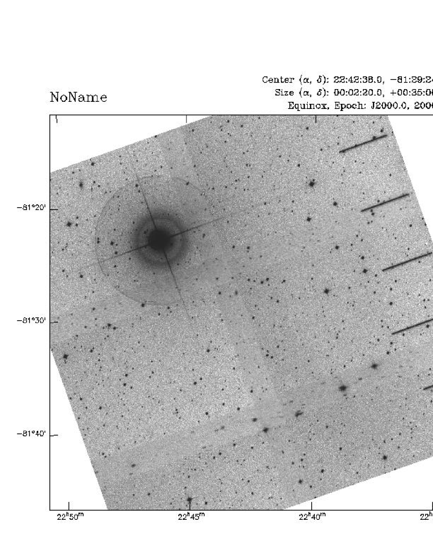
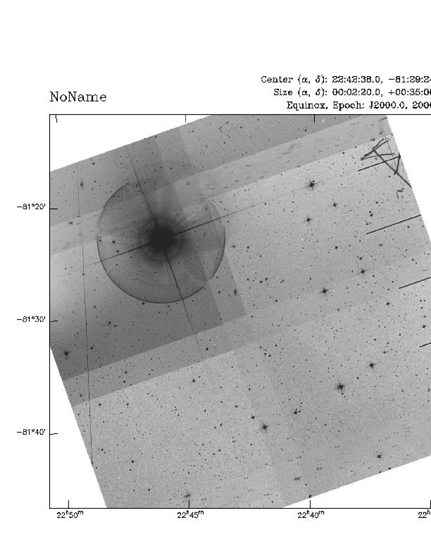
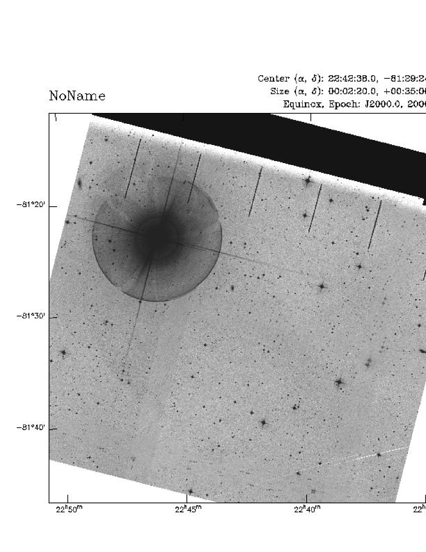
Figure 1: Subimages of three of the nine scanned plates that overlap a small patch of sky centered around (RA,Dec)=(341.8, -81.4) deg (J2000) from which part of USNO-B Catalogwas created, retrieved from the US Naval Observatory Precision Measuring Machine Data Archive. Note the different orientations of the diffraction spikes generated by brighter stars, and the multiple halos surrounding the brightest star.

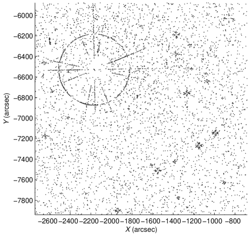
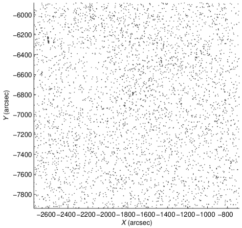
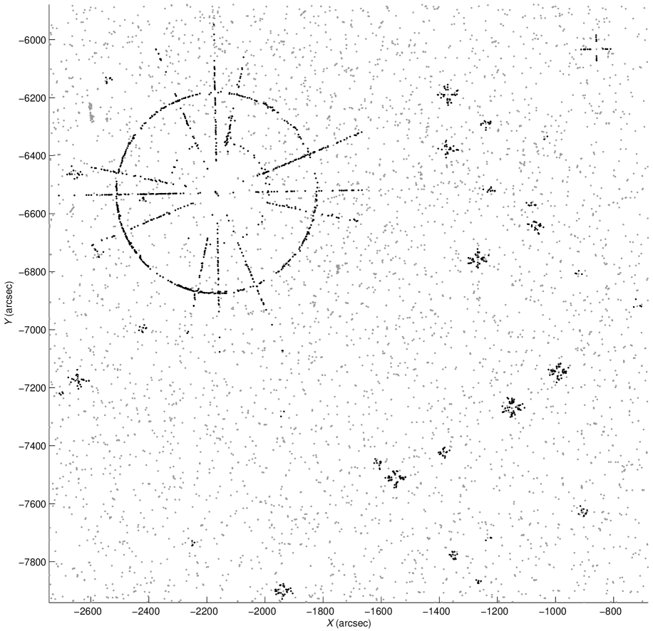
Figure 2: The same small patch of sky as pictured in Figure 2, taken from the USNO-B Catalog, in tangent-plane coordinates relative to a tangent point at the center of the containing healpixel, in units of $\mathrm{arcsec}$. The bright stars in this patch have multiple sets of diffraction spikes because they lie in a sky region where plates taken at different orientations overlap. Upper left panel: All USNO-B Catalog entries in this patch. Right panel: The same patch with dark points showing catalog entries marked as spurious by either the diffraction spike or reflection halo criteria described in the text. Lower left panel: The same patch, with only non-spurious entries shown.

The diffraction-limited point-spread function of a physical telescope is related to the Fourier transform of the entrance aperture. In this transform, the thin cross-like support structure holding the secondary mirror in the entrance aperture produces a large cross-like pattern in the stellar point-spread function (PSF). The sources automatically extracted from the scans of the photographic plate images include many spurious features that are in fact just detections of these diffraction spikes (Figures 1 and 2).

The survey cameras that took the imaging data used to construct the USNO-B Catalog are on equatorial mounts and have no capability for rotation of the support structure relative to the sky once the pointing of the telescope is set. The diffraction spikes for any two images taken by the same camera at the same pointing are therefore always aligned. For this reason, spurious stars detected as part of one of these spikes in one image in one band often line up with spurious stars detected in the corresponding spike in some other band. Some spurious “spike” catalog entries thereby satisfy the USNO-B Catalog vetting requirement that catalog entries have cospatial counterparts in multiple bands.

Fortunately, spurious spike entries can be identified on the basis of morphological regularities in the two-dimensional distribution on the sky of the spurious catalog entries they generate. These regularities include the following: (1) Diffraction spikes are centered on bright ($<13\,\mathrm{mag}$) stars. In what follows, the central star for a diffraction spike will be referred to as the “generating star”. (2) Because telescope supports are usually four perpendicular rods, each diffraction spike generated by a bright star has four lines at right angles to one another. (3) The diffraction spike brightness is proportional to the brightness of the generating star, but each spike becomes fainter with angular distance from the generating star. Given that sources extracted from the scanned plates are detected to some limiting brightness, the angular length of a diffraction spike is closely related to the magnitude of the generating star (Figure 5). (4) The angular width of a diffraction spike is narrow, so the two-dimensional density of spurious spike entries can be very large. The angular width is set by physical optics and is therefore roughly independent of the magnitude of the generating star. (5) The orientation of the diffraction spike pattern is roughly common to all spikes taken by the same camera at the same pointing. We can use the regularities among diffraction spikes to guide a sensitive, automated search.

Each USNO-B Catalog entry is tagged with a survey identifier and one or more field numbers corresponding to the plates in that survey in which it was detected. Because all diffraction spikes in one field will share the same orientation and properties, we analyze the USNO-B Catalog entries one field at a time. In this context, we consider an entry to belong to a particular field if any of its photometric measurements has been given that field number.

2.2 Reflection halos

The brightest stars in the USNO-B Catalog are surrounded not just by diffraction spikes but by a thin circular ring or “halo”. This halo is caused by internal reflections in the camera. Because this has a geometric-optics rather than a physical-optics origin, the halo radius is not a function of the wavelength of the imaging bandpass. This means that spurious “halo” catalog entries can easily be present and cospatial in multiple bands and thereby pass the USNO-B Catalog vetting process (Figures 1 and 2).

Again, the spurious catalog entries can be identified by the patterns they make on the sky. Regularities include the following: (1) Halos are centered on extremely bright ($<7\,\mathrm{mag}$) generating stars. (2) Halos have a circular or near-circular shape. (3) Because they are very thin in the radial direction, spurious halo entries have high two-dimensional density on the sky. (4) The spurious halo entries are usually close to making up full circles, and only rarely appear in just a fragment of a circle. These regularities permit a sensitive search.

2.3 Other spurious entries

In addition to the spikes and halos we address above, there are other categories of spurious catalog entries with other origins, including but not limited to the following: (1) There are some lines of entries from fortuitously coincident features (scratches, trails, handwriting, and other artifacts) on overlapping plates. (2) There are some duplicate entries for individual stars in sky regions where two fields overlap. These are cases in which individual stars detected in multiple fields have not been correctly identified as identical. (3) There are quasi-spurious clusters of entries in and around extended objects such as galaxies, nebulae, and globular clusters.

We are doing nothing about any of these spurious features, in part because they do not have regularities that lend themselves to computer-vision techniques we employ in finding the previously mentioned defects. They also represent a much smaller fraction of the USNO-B Catalog entries than the spurious entries from diffraction spikes and reflection halos.

Of course the USNO-B Catalog contains also many entries that are in fact compact galaxies rather than stars. However, these entries are not spurious from our perspective, since compact galaxies are as good as—or better than—stars for our Astrometry.net astrometric calibration efforts, and most other astrometric calibration tasks.

3 Methods

The Catalog we begin with is not the unmodified USNO-B Catalog, but rather the USNO-B Catalog with the Tycho-2 Catalog (Høg et al, 2000) stars re-inserted by us from the official Tycho-2 Catalog release. We were forced to perform this operation because in the official USNO-B Catalog release, the Tycho-2 Catalog stars were added in an undocumented binary format.

3.1 Diffraction Spikes

We begin by dividing the Catalog into a fine healpix (Górski et al, 2005) grid, and projecting the entries in each healpixel onto planes tangent to each healpixel’s center. For each entry we calculate the average $m$ of all magnitudes of all bands in which the entry has been detected, and we find the union of all fields in which the entry is present.

For each field present, we construct a “profile” of the field’s largest diffraction spikes, by overlaying the local neighborhoods of the ten brightest stars in the field. Given the regularities discussed above, we can expect all spikes in each field to have the same orientation. Therefore, each composite profile has one dominant orientation, which is more apparent than in any single star’s neighborhood. To find each field’s orientation, we first convert the composite profile into polar coordinates, collapse the angles of each point into a ${\pi\over 2}\,\mathrm{rad}$ range, and calculate a rough histogram of the resulting angles. The angle with the most densely populated bin is used as an initial guess of the field’s orientation, which is then re-estimated using an iteratively reweighted least squares (IRLS) fitting algorithm for robust M-estimation (Hampel et al, 1986). The M-estimation is guaranteed to converge to an estimate of the orientation that locally minimizes a total cost $\sum_{k}\rho(e_{k})$ where $e_{k}$ is the angular distance of entry $k$ from the estimated orientation. We employ a Geman-McLure (GM) cost function $\rho(e_{k})=e_{k}^{2}/(\sigma^{2}+e_{k}^{2})$, where $\sigma$ is the initial guess of the root-variance of the angular width of a spike. This GM cost function replaces the standard least-squares cost function $\rho(e_{k})=e_{k}^{2}/\sigma^{2}$ and thereby downweights outliers. The resulting angle is a very robust and precise estimate of the average orientation of all diffraction spikes present in the field.

We iterate over fields, using our estimation of each field’s dominant orientation to rotate the entries present in each field such that the diffraction spikes present become axis-aligned on average, making their detection much easier. Because there is sometimes some discrepancy between the position of the diffraction spike’s generating star and the center of the diffraction spike, we perform a robust estimation of the centerpoint of the spike, just as we did in estimating the orientations of the field profiles. With the diffraction spike axis-aligned and zero-centered, we collapse all of the entries in the neighborhood of the diffraction spike into a single composite of all four “corners” (as if we were to convert the neighborhood to polar coordinates, and collapse their angles into a ${\pi\over 2}\,\mathrm{rad}$ range), thereby reducing the four-part diffraction spike to a single dense cluster of points.

We found a power-law approximation to the relationship between the magnitude of the generating star and the angular extent of the diffraction spike it generates among spurious entries. This was found by initially hand-labeling a small subset of the data, making a crude fit to the hand-labeled data, then later refining the estimate using the results of our algorithm. Given the magnitude of a generating star, we are able to use this relationship to estimate the angular extent of the spike we would expect that generating star to produce. As previously mentioned, the width of each spike is roughly independent of the magnitude of the generating star, and is therefore initialized to a constant value. This estimate of the center and extent of the spike is used to initialized a two-dimensional Gaussian, which is then fit to the entries belonging to the diffraction spike using iterated variance clipping at 2.5 sigma. What we construct is not a traditional multivariate normal distribution, which would assume that the data lies in an elliptical distribution, but is instead a “rectangular” distribution. That is, we consider an entry to be within the Gaussian distribution if it is simultaneously within 2.5 sigma of the width and 2.5 sigma of the length of the distribution. When the Gaussian converges to its final parameters, we take the rectangular area within 2.5 sigma, and extend its range towards the generating star to cover all entries between the area and the generating star at the center of the spike. If this area’s angular width, length, and position all pass a set of thresholds, detailed later, we flag all of the entries within it (excluding the generating star and any Tycho-2 stars, which we assume are not spurious) as potential spurious entries. If these entries pass a set of thresholds (detailed below) they are marked as spurious.

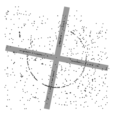
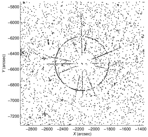
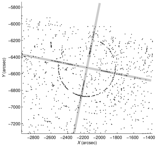
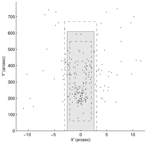
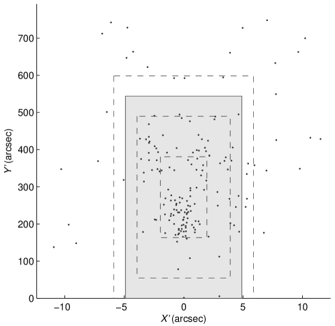
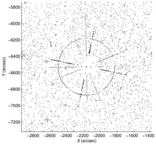
Figure 3: A narrative demo of finding a single spike within the patch of sky shown in Figure 2. Upper left panel: The composite profile of the current field, with the field’s estimated orientation highlighted. The profile is dominated by the spike of the current generating star, which is the largest in the field. Upper center panel: The neighborhood surrounding the current generating star, with all entries in all fields shown. Upper right panel: The same neighborhood, with only entries in the current field shown. The dominant orientation from this field’s composite profile is highlighted. Lower left panel: All four directions of the spike, collapsed into one ${\pi\over 2}\,\mathrm{rad}$ profile. The dashed lines outline the areas encompassed at 1, 2, and 3 times the root-variance of the Gaussian used to initialize the variance clipping. The solid rectangle is the area encompassed at 2.5 sigma, which is threshold for flagging entries. The solid rectangle is extended all of the way to the bottom, as it is assumed that all of the spike profile between the spike cluster and the generating star is also spurious. Lower center panel: The same profile, after the Gaussian has been fit using variance clipping. The solid rectangle shown here is the final area we use for determining if entries are flagged. Lower right panel: The neighborhood surrounding the generating star with all entries shown, and with the newly-flagged spike entries darkened. The diffraction spikes in the other orientations come from different fields and are flagged by later passes of the algorithm.

The algorithm is depicted in Figure 3.

3.2 Reflection halos

Once all spurious catalog entries attributed to spikes are found and temporarily removed (such entries disturb the results of the halo detection algorithm), we search the remaining catalog for halos. This process is similar to the process of searching for diffraction spikes: We divide the Catalog into a fine healpix grid and process each grid cell independently. We project the entries in each grid cell onto a plane tangent to the cell’s center. Next, we examine each star brighter than $7\,\mathrm{mag}$, and attempt to find and eliminate halos that it has generated. Since the radius of each halo is not dependent on the magnitude of its generating star, the size of the neighborhood we search is constant.

We convert each neighborhood into polar coordinates centered at the generating star, and calculate a histogram of the radii of all entries in the neighborhood. This simple count of the number of stars present at different radii is used to generate a more informative histogram of the densities of stars at each radius. Our initial guess of the radius of the halo is whichever coarse bin is the most dense.

With this estimate of the radius of our halo, and with a constant as our initial estimate of the radial width of the halo, we construct a one-dimensional Gaussian and again robustly fit the position and width of the Gaussian using variance clipping at 2.5 sigma. Once the re-estimation has converged, we check that our resulting values for the variance of the width are reasonable ($<3\,\mathrm{arcsec}$), and if so, we label all entries within 2.5 sigma of the Gaussian as potentially spurious. Again, if these entries pass another set of thresholds, they are marked as spurious.

Because one generating star may produce multiple halos, we search each generating star, and remove each salient halo we find, until we fail to detect any new halo that passes our thresholds.

3.3 Parameters of the Algorithms

By necessity the algorithms have a number of free parameters. Some of these are measurements of diffraction-spike and reflection-halo configurations, derived from quantitative analyses of the properties of the spurious entries, while others are additional conservative constraints, applied to ensure that the spurious entries appear to be correctly identified on visual inspection of the results.

In addition to the parameters that specifically apply to the spike and halo identification algorithms, we somewhat arbitrarily chose to work in a $N_{\mathrm{side}}=9$ healpix grid; there are $12\times 9\times 9=972$ healpixels. We set all variance-clipping thresholds to 2.5 sigma, and when we define regions by variance clipping we make them 2.5 sigma in half-width.

3.3.1 Measured Spike Parameters

• We search for diffraction spikes generated by stars brighter than $13\,\mathrm{mag}$. Bright stars tend to produce large diffraction spikes containing many spurious entries, while dimmer stars produce small diffraction spikes containing few, and potentially ambiguous, spurious entries. When we extended our search to stars brighter than $15\,\mathrm{mag}$, we found that the proportion of falsely labeled spurious entries increased dramatically. Our decision to restrict to $<13\,\mathrm{mag}$ is further supported by the second panel of Figure 4, which shows that generating stars at $>13\,\mathrm{mag}$ have mean number of entries per spike less than four, which means that most will contain too few entries to be accepted.

• Our initial estimate of the angular length $\ell$ of a diffraction spike given the magnitude $m$ of its generating star is $\ell=3500\times 1.53^{-m}\,\mathrm{arcsec}$; see Figure 5. This estimate initializes a refinement by iterated variance clipping and therefore does not strongly affect our results. In detail this relationship between length and magnitude depends on band, exposure time, and data quality, and is is therefore different for every plate; but since we use it only as an initialization, those details do not substantially affect our results.

• Our initial estimate of the angular width of a spike is $1\,\mathrm{arcsec}$. This also initializes a refinement by iterated variance clipping and also has little effect on our results.

• We define the “reasonable” width of a diffraction spike to be three times the initial estimate of $1\,\mathrm{arcsec}$. If the adaptive fitting process produces a width larger than this, the candidate spike is rejected.

3.3.2 Additional Spike Constraints

• The size of the local neighborhood constructed around each spike is $2.5$ times the initial estimate of the spike’s size. This limits the catalog entries considered in the subsequent analysis, though the effect on our results is minimal.

• We required each spike to have entries in at least $2$ of the $4$ spike regions.

• We required the total area within the four spike regions to be at least as dense in Catalog entries as the surrounding area.

3.3.3 Measured Halo Parameters

• We search for halos around generating stars brighter than $7\,\mathrm{mag}$. Our experiments have shown that halos do not appear around stars dimmer than this.

• We discard any halo whose radius is outside the range of $240$ to $410\,\mathrm{arcsec}$. Direct inspection of the catalog shows that reflection halos rarely appear outside of this range.

• Our initial estimate of the standard deviation of the radial width of a halo is $1.8\,\mathrm{arcsec}$. This is approximately the average value to which our variance-clipping fitting algorithm converges.

• We discard any halo for which our variance-clipping fitting algorithm computes a radial width larger than $4.5$ times the initial estimate.

3.3.4 Additional Halo Constraints

• Each halo must contain at least $25$ catalog entries.

• The density of catalog entries in each halo annulus must be at least $1.25$ times the density of the area near the halo.

• There must be entries present in the halo annulus every ${\pi\over 4}\,\mathrm{rad}$. This forces all detected halos to be fully circular, rather than just fragments of circles. More importantly, this requirement prevents the false detection of halos near the edges of healpixels, which would otherwise happen very often. Unfortunately, this requirement prevents us from detecting any halo near the edges of a healpixel.

3.4 Limitations

Limitations of our procedures include the following.

• The algorithm assigns hard labels to indicate that an entry is spurious. A future version of the algorithm could assign an assessment of our confidence that an entry is spurious.

• The algorithm processes each healpixel independently, and we have not included a buffer region around the edges of the healpixels, so there are minor edge effects: the algorithm is less likely to detect spurious entries near the healpixel boundaries. We expect this to affect roughly $0.4\,\mathrm{percent}$ of the diffraction spikes and $3.5\,\mathrm{percent}$ of the reflection halos.

• The algorithms are highly specialized to the typical data in the USNO-B Catalog. If a small fraction of the data in the Catalog come from some telescope with, for example, three rather than four supports for the secondary, or very different internal reflections, the algorithms we use would not detect the spurious features in those data.

• There are many hard settings of parameters, as discussed above. Most of these are either just initializations for iterative procedures or else set manually after an analysis of the data, but more experimentation could have been performed if we had a substantial data set in which the spurious entries had been reliably identified in advance.

• Sometimes a diffraction spike that exists in multiple fields is detected in a field whose orientation does not match the spike’s orientation as well as some other field. The is because the order in which we search each field is arbitrary; we flag a detected diffraction spike upon it’s first successful detection. This usually results in a detected diffraction spike with an unusually wide angular width. Though this happens frequently, its overall effect on the fidelity of our results is small. A better solution would be to remove spikes in non-increasing order of their resemblance to our model of a diffraction spike.

• We ought never consider as a generating star any star that was marked spurious in the analysis of a brighter generating star. We don’t currently enforce this, and it may produce some incorrect identification of spurious entries.

• Many of these limitations could be overcome if we constructed a complete generative model of diffraction spikes and halos. This would allow us to “score” potential spurious detections with something approaching a probability that they are spurious, rather than simply cut at hard thresholds. This could also improve the fidelity of our results, by allowing us to increase our statistical requirements of some parameters of our generative model when a detected spike or halo fails to fit other parameters. For example, if a possible halo appears at an uncommon radius, a proper generative model would effectively put a stronger constraint on other properties (such as the density of entries in the halo annulus) in order for the entries to be marked as spurious with high probability. Done well, this approach could also allow us to reduce the number of individual requirements we require of each detected spike and halo. This would be aided by a set of hand-labeled spikes and non-spikes, with which we could tune the generative model — or which we could use as input to some kind of discriminator which would tune the model automatically.

4 Results

The number of entries flagged as spurious on diffraction-spike grounds is 24,148,382 ($2.3\,\mathrm{percent}$ of the USNO-B Catalog) and on halo grounds is 196,133 ($0.02\,\mathrm{percent}$). Our grounds for declaring an entry spurious are conservative in the sense that a spike or halo is only treated as being detected if it passes a set of statistical thresholds.

The method works by marking as spurious all USNO-B Catalog entries in a set of finite regions of the sky, with those sky regions adaptively fit to the observed diffraction spike and reflection halo features. Because the total solid angle removed is non-zero, we expect some of the entries we mark as spurious to in fact correspond to real sources. We can estimate this in a representative healpixel: Healpixel 0 contains $299573$ USNO-B Catalog entries; we flag as spurious $7924$ entries within a set of regions comprising $1.5\times 10^{-5}\,\mathrm{ster}$ ($0.12\,\mathrm{percent}$ of the healpixel); we expect therefore some 300 of these to correspond to real stars. We tested this hypothesis with the 2MASS PSC Catalog. In this healpixel there are $81089$ entries, of which we would expect $\sim 100$ to lie in the spurious area we’ve removed. We find that $82$ 2MASS PSC Catalog entries match to a spurious USNO-B Catalog entry and no non-spurious USNO-B Catalog entry, consistent with what we would expect assuming a uniform distribution of 2MASS PSC Catalog entries over the healpixel. This count is probably an overestimate, because there are some diffraction artifacts in the 2MASS PSC Catalog that are similar to those in USNO-B Catalog. Our marking of spurious entries is aggressive in this sense; as we noted in the Introduction, this is because for our scientific purposes we require a catalog as clean of spurious entries as possible.

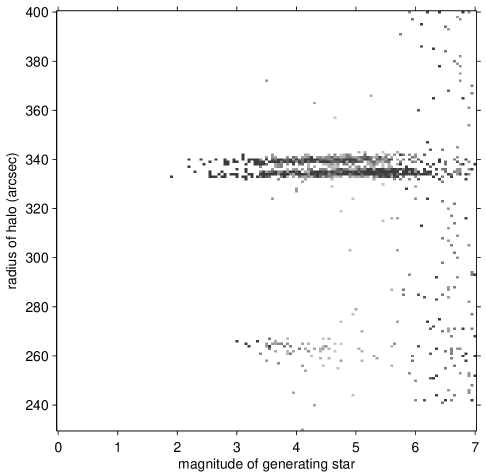
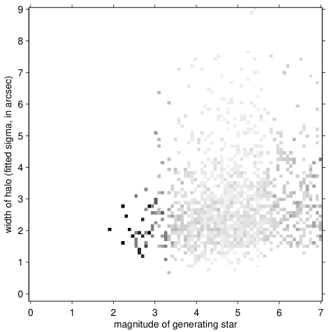
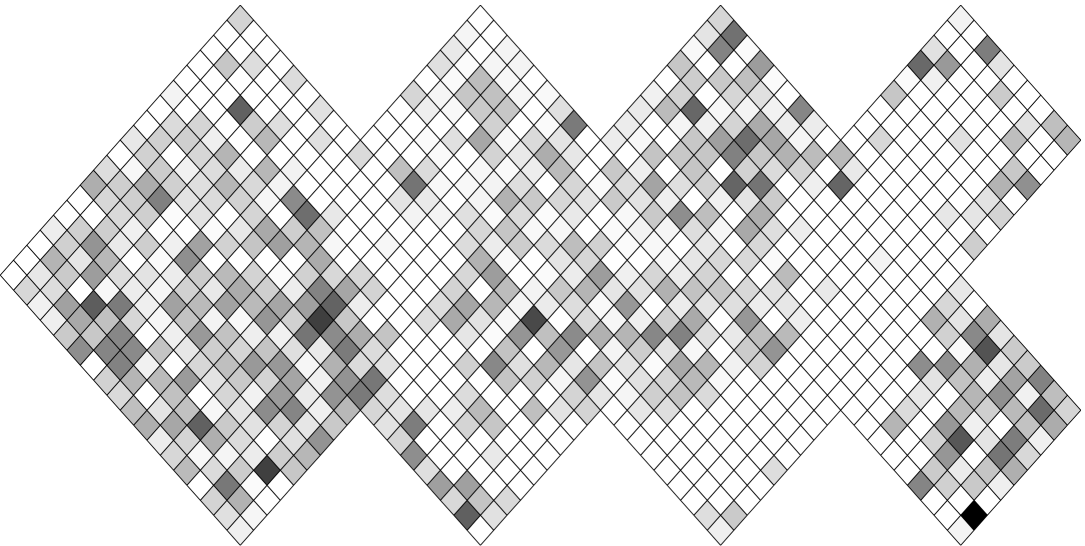
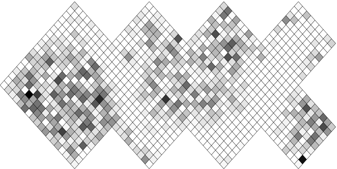
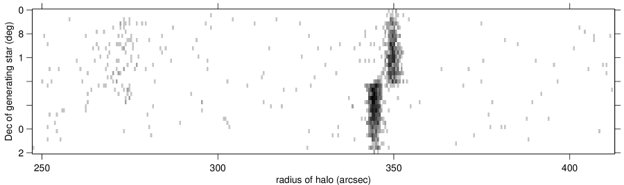
Figure 6: Regularities of spurious catalog entries identified as caused by reflection halos. Top-left panel: Two-dimensional histogram showing adaptively fit reflection-halo radii as a function of generating star magnitude. Each vertical column of the histogram has been independently normalized. Top-right panel: Similar two-dimensional histogram but showing the adaptively fit widths of the halo annuli. Middle-left panel: Two-dimensional solid-angular density on the sky of spurious entries identified as parts of reflection halos. The darker a healpixel is, the more spurious “halo” entries it contains. Middle-right panel: The same but shown relative to the number of catalog entries in that healpixel. Wide bottom panel: Two-dimensional histogram showing that each of the two principal halo radii is in one hemisphere of the sky.

Properties of the spurious entries we have identified are shown in Figures 4, 5, and 6, including the numbers and fractions of spurious entries as a function of generating star magnitude, and distributions of spikes and halos in size and on the sky. These figures show a number of important regularities, for example that brighter stars have larger diffraction spikes (as expected), that the widths of the spikes is not a function of generating star magnitude (also as expected), and that both the number of spurious entries and our ability to robustly detect them are functions of sky position (mainly because of the Galactic Plane). Figure 6 shows that there are two different dominant halo radii, one for the North and one for the South; presumably this indicates differences in the hardware used for each hemisphere.

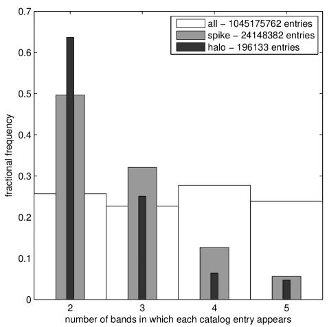
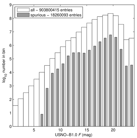
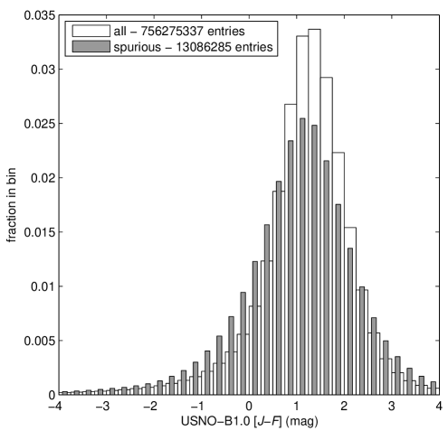
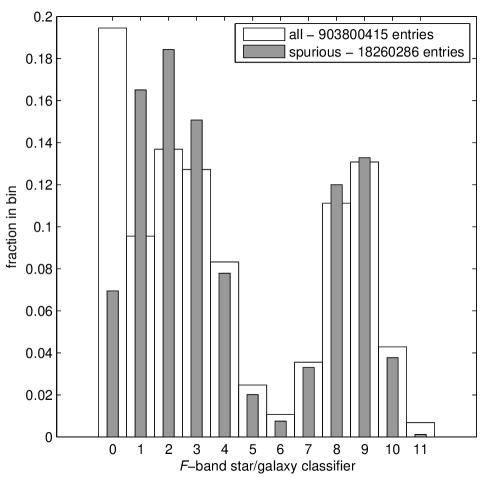
Figure 7: Spurious catalog entries are not obvious from their basic photometric properties. Top-left panel: Number of the five bands in the merged Tycho-2 and USNO-B Catalogs in which entries show detections, for all and spurious entries. Top-right panel: Magnitude distribution, for all and spurious entries with detections in the $F$ band. Bottom-left panel: J-F color distribution, for all and spurious entries with detections in the $J$ and $F$ bands. Bottom-right panel: USNO-B Catalog $F$-band star-galaxy separator quantity, for all and spurious entries with detections in the $F$ band.

At the outset, we imagined that we could remove these spurious entries trivially using the photometric properties listed in the Catalog. For example, there is no reason in principle that a spurious entry would obtain a reasonable color or pass star–galaxy separation. In Figure 7, we show the distribution of the spurious entries in photometric properties such as magnitude, color, and star–galaxy separation. This Figure shows that it would not have been possible to identify the spurious on photometric grounds, including even the number of images with detections. Presumably the reasonable colors and large numbers of overlapping images in which the stars are detected result from the great stability of the hardware and software employed in the construction of the USNO-B Catalog. It would have been extremely difficult to reliably identify the spurious entries without automatic computer-vision techniques like those employed in this project.

Associated with this paper is a small amount of computer code, the information required to clean the USNO-B Catalog of the spurious entries we identified, and some methods for accessing our cleaned version of the USNO-B Catalog. All of these are available at the Astrometry.net web site.

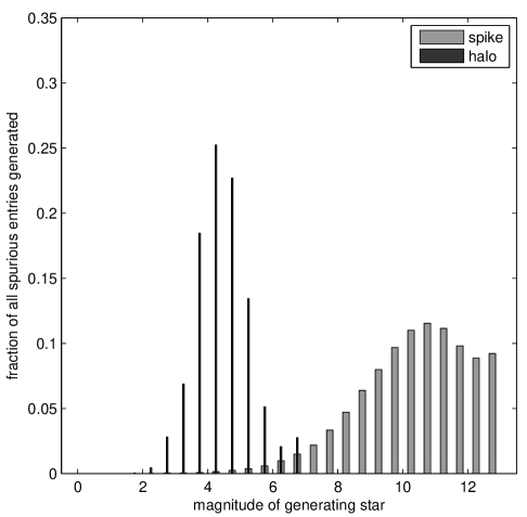
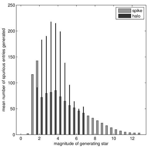
Figure 4: Statistics of spurious entries. Left panel: The fraction of all entries marked as spurious as a function of generating star magnitude. Right panel: The mean number of entries marked as spurious per generating star as a function of generating star magnitude.

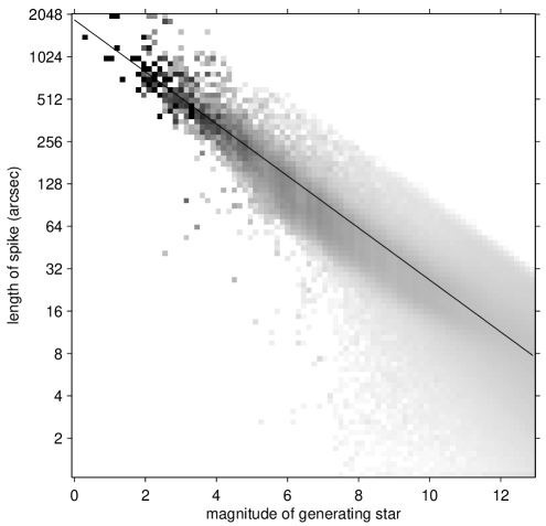
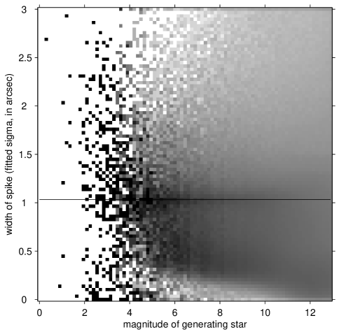
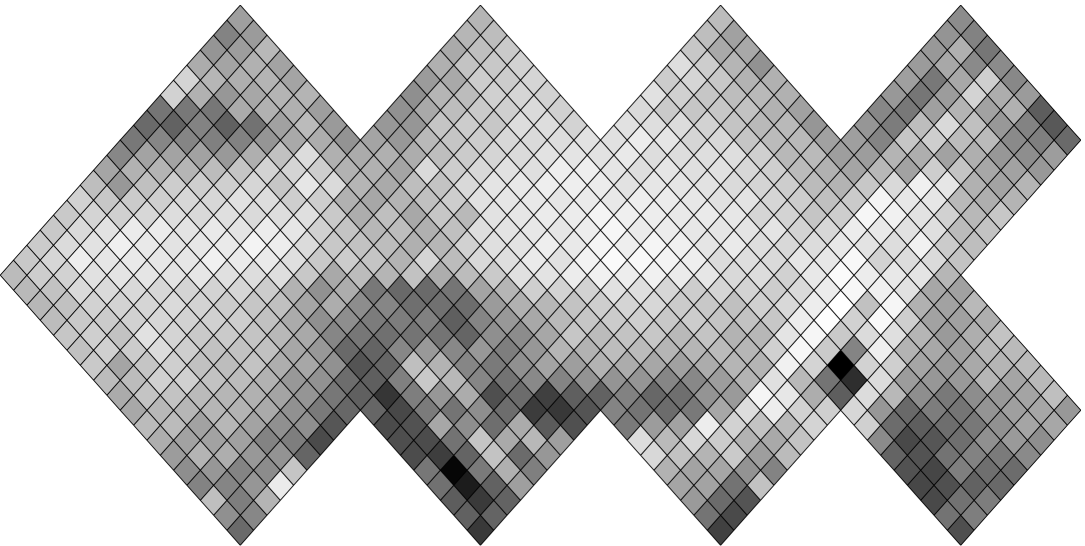
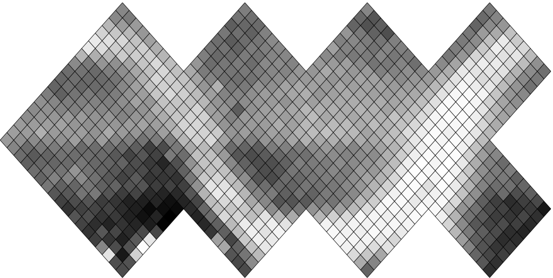
Figure 5: Regularities of spurious catalog entries in the USNO-B Catalog identified as caused by diffraction spikes. Top-left panel: Two-dimensional histogram showing the adaptively fit radial lengths of the spikes, found by iterative variance-clipping, as a function of generating star magnitude. Each vertical column in the histogram is independently normalized. The solid line shows the value used to initialize the adaptive fitting. Top-right panel: Similar two-dimensional histogram but showing the adaptively fit widths of the spikes, as a function of generating star magnitude. The solid line shows the initial value. Bottom-left panel: The two-dimensional solid-angular density on the sky of spurious entries identified as parts of diffraction spikes as a function of sky position (shown as an “unwrapped” $N_{\mathrm{side}}=9$ healpixel grid). The darker a healpixel is, the more spurious “spike” entries it contains. Bottom-right panel: The same, but shown relative to the number of catalog entries in that healpixel. In the two sky density plots, a North–South asymmetry is visible, as well as the Galactic plane.

References

- Górski et al (2005) Górski, K. M., Hivon, E., Banday, A. J., Wandelt, B. D., Hansen, F. K., Reinecke, M., & Bartelmann, M., 2005, ApJ, 622, 759
- Hampel et al (1986) Hampel, F. R., Ronchetti, E. M., Rousseeuw, P. J., & Stahel, W. A., 1986, Robust Statistics: The Approach Based on Influence Functions, Wiley, New York
- Høg et al (2000) Høg, E., et al, 2000, A&A, 355, L27
- Lang et al (2007) Lang, D., Hogg, D. W., Mierle, K., Blanton, M., & Roweis, S., 2007, Science, submitted
- Monet et al (2003) Monet, D. G., et al, 2003, AJ, 125, 984
- Storkey et al (2004) Storkey, A. J., Hambly, N. C., Williams, C. K. I., & Mann, R. G., 2004, MNRAS, 347, 36