Unbiased sampling of globular lattice proteins in three dimensions

Abstract

We present a Monte Carlo method that allows efficient and unbiased sampling of Hamiltonian walks on a cubic lattice. Such walks are self-avoiding and visit each lattice site exactly once. They are often used as simple models of globular proteins, upon adding suitable local interactions. Our algorithm can easily be equipped with such interactions, but we study here mainly the flexible homopolymer case where each conformation is generated with uniform probability. We argue that the algorithm is ergodic and has dynamical exponent $z=0$. We then use it to study polymers of size up to $64^{3}=262\,144$ monomers. Results are presented for the effective interaction between end points, and the interaction with the boundaries of the system.

Self-avoiding random walks of various types are ubiquitous in Nature and often serve as a first step in modeling polymeric systems deGennes . In a good solvent, polymers assume spatially extended conformations which are well described by the usual Self-Avoiding Walk (SAW) model. In this model, each monomer is assigned a fugacity $\beta$, and the SAW is recovered at the smallest value $\beta_{\rm c}$ of $\beta$ so that the mean length of the walk diverges. This is a critical point, meaning that observables exhibit power law behaviors that are independent of the precise microscopic model. Therefore, the latter is conveniently defined on a hypercubic lattice in $d$ dimensions.

By contrast, proteins in their native globular state assume compact confirmations that occupy space as densely as possible. This suggests modeling such biopolymers as Hamiltonian Walks (HW); by definition these are self-avoiding walks which are constrained to visit each of the lattice sites exactly once. Upon adding further local interactions, the HW model has been proposed as a description of protein melting Flory (with bending rigidity), or of protein folding Dill (with suitable interactions among amino acids). The simplest example of the latter is the so-called HP model in which only two types of amino acids (Hydrophobic or Polar) are taken into account.

In $d=2$ dimensions an amazing number of exact results on self-avoiding walk models are known, due in particular to the application of Conformal Field Theory (see review for a recent review). For instance, both the HW model and the Flory model of protein melting have been solved KondevCFT . But in the physically more relevant case of $d=3$, such exact results are not available, and one must resort to approximate techniques, or to numerics, to extract information about the model at hand.

Much work on such lattice proteins is based on exact enumeration studies in which all possible conformations on a small cube of size $N=L\times L\times L$ are generated. Unfortunately, despite of the HW constraint, the number of conformations is so large that even the case $L=4$ is out of reach Pande . Needless to say, such small sizes are very sensitive to the peculiarities of the lattice model (e.g., the choice of lattice), and cannot be considered representative of real proteins.

Therefore, an efficient and unbiased importance sampling scheme of the Monte Carlo (MC) type would be most welcome to study larger $L$ and make precise statements about the thermodynamic limit $L\to\infty$. For the usual SAW case, this is furnished by the so-called pivot algorithm pivot . In each move, a randomly chosen lattice symmetry is applied to the part of the walk subsequent to a randomly chosen pivot point. The move is accepted if the resulting walk is self-avoiding. For $N\to\infty$, the acceptance ratio goes to zero, but the few accepted moves suffice to decorrelate the system in time $\sim N$. But in the HW limit, the acceptance ratio becomes identically zero, and so the pivot algorithm is useless in this case. Alternative growth-type algorithms are not guaranteed to yield unbiased sampling Zhang .

In this Letter we propose an MC algorithm which is specifically adapted to HW, and we test it in details for the $d=3$ flexible homopolymer case. We show that it satisfies detailed balance and give evidence for ergodicity; each conformation is therefore generated with uniform probability. In contrast to the pivot algorithm, each move is accepted with probability one. One move takes time $\sim N$, and $N$ moves are sufficient to completely decorrelate the system. Using our algorithm, we generate conformations of size $N=262\,144$ monomers with ample statistics, and give a number of results on their geometrical properties.

Algorithm. Let ${\cal C}$ be a Hamiltonian walk on the cubic lattice. Choose one of its two end points randomly and uniformly; call it ${\bf x}$. Note that site ${\bf x}$ is adjacent to one occupied and five empty links. Choose one of the five empty links with uniform probability; call it $({\bf x}{\bf y})$. Then among the occupied links adjacent to ${\bf y}$ there is exactly one which forms part of a loop in ${\cal C}\cup({\bf x}{\bf y})$; call it $({\bf y}{\bf z})$. [Note that if ${\bf y}$ is the other end point of ${\cal C}$ there is one occupied link adjacent to ${\bf y}$; otherwise there are two.] Change ${\cal C}$ by adding $({\bf x}{\bf y})$ and removing $({\bf y}{\bf z})$.

Figure 1: Move between two of the $2\,480\,304$ possible Hamiltonian walks on a $3\times 3\times 3$ cubic lattice.

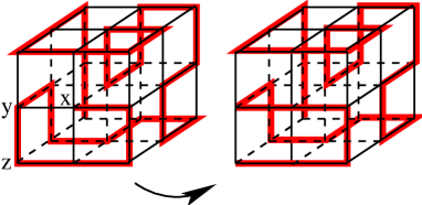
The MC move just described is illustrated in Fig. 1. It was studied in two dimensions in Oberdorf . In what follows we choose the system to be confined to an $L^{3}$ cube with free (i.e., non periodic) boundary conditions. A small modification is then needed if ${\bf y}$ is outside the cube. In that case, the move consists in leaving ${\cal C}$ unchanged.

Unbiased sampling. The above move clearly satisfies detailed balance. To prove that it is also ergodic it suffices to show that any ${\cal C}$ can be transformed into a fixed reference configuration ${\cal C}_{0}$ in a finite number of moves. Let ${\cal C}_{0}$ be one of the two configurations with a maximal number of occupied horizontal links. One may approach ${\cal C}_{0}$ by choosing always ${\bf y}$ so that $({\bf x}{\bf y})$ is horizontal. Unfortunately, $({\bf y}{\bf z})$ may also turn out to be horizontal, so positive progress is not made in every step. Moreover, if both end points end up on the left or right side of the cube, and are both adjacent to an occupied horizontal link, one will actually have to remove a horizontal link to proceed. Due to these complications we cannot prove ergodicity for arbitrary size $L$.

However, we can argue in favor of ergodicity by testing it for small lattices. Using exact enumeration techniques, we find that there are $2\,480\,304$ HW on an $L=3$ cube enumeration , and our MC algorithm generates all of them. We also find that there are $3\,918\,744$ Hamiltonian Circuits (HC), or closed walks, on a $3\times 3\times 4$ parallelepiped enumeration . A HC can be formed from a HW whose end points are nearest neighbors on the lattice, by adding the missing link. In this way we have checked that all $3\,918\,744$ HC can be generated as well. Similar checks have been made on smaller parallelepipeds.

Assuming that ergodicity holds in general, we conclude that the MC process converges towards the equilibrium distribution, i.e., that all Hamiltonian walks are sampled with uniform probability.

Performance. Identifying the correct edge $({\bf y}{\bf z})$ to be removed necessitates tracing out the loop formed when adding ${\bf x}{\bf y}$, and so one move takes a time $\sim N$. But note that when the end point moves from ${\bf x}$ to ${\bf z}$, the part of the chain $[{\bf x}{\bf z}{\bf y}]$ is reversed and becomes $[{\bf z}{\bf x}{\bf y}]$. Thus, if one were to use the algorithm to study a heteropolymer problem, the sequence of amino acids on that part would have to be reversed as well. So in that respect, and in terms of chain connectivity, the move is certainly more non-local than it looks at first sight.

Define now the autocorrelation function $G(t)$ as the link overlap function with respect to some reference initial configuration. The time $t$ is measured in units of MC moves per site, and averages are done over $100$ independent runs. We have measured $G(t)$ for system sizes $L=4,8,16,32$ and found that it decays exponentially towards an $L$-dependent constant, which can be determined numerically by averaging $G(t)$ over the last 100 time units in a sufficiently long simulation. Subtracting this constant, and rescaling, gives a normalized autocorrelation function $\tilde{G}(t)$ satisfying $\tilde{G}(0)=1$ and $\tilde{G}(t)\to 0$ as $t\to\infty$. Defining now the autocorrelation time $\tau$ by $\tilde{G}(t+\tau)=\frac{1}{2}\tilde{G}(t)$, we estimate $\tau$ by averaging over the first $4\tau$ of the simulation. For the system sizes mentioned this gives $\tau=1.33$, $1.27$, $1.20$, and $1.15$. This fits nicely as $\tau\sim L^{z}$ with dynamical exponent $z=-0.024\pm 0.001$. Of course we cannot have $z<0$, since one MC move changes only a finite number (two) of links. We therefore conclude that $z\approx 0$.

Simulations. We have generated conformations on lattices up to size $L=64$ (i.e., $262\,144$ monomers) with ample statistics. In all cases, the first $t=100$ MC moves per site were discarded. The various averages and histograms were then made over $T$ MC moves per site, with measurements being made after each individual MC move. We have taken $T=10^{6}$ for $L\leq 20$, $T=10^{5}$ for $20<L\leq 30$, $T=10^{4}$ for $30<L\leq 40$, $T=10^{3}$ for $40<L\leq 60$, and $T=10^{2}$ for $L>60$. Data were generated for both even and odd $L$ in order to detect any parity effects.

Asymptotic isotropy. We have measured the histogram for the end-to-end distance vector ${\bf x}_{12}=\pm({\bf x}_{1}-{\bf x}_{2})$; note that the sign is immaterial because of the indistinguishability of the end points. Not all values of ${\bf x}_{12}$ are possible, since for $N$ even (resp. odd) the end points must belong to different (resp. identical) sublattices by an easy parity argument.

We first checked for $L=4$ that the histogram is isotropic on the microscopic level. Thus, for each ${\bf x}_{12}$ respecting the parity constraint, the 6, 8, 12 or 24 vectors related to it by lattice symmetries are found to be generated with the same frequency (up to counting statistics fluctuations).

Still, vectors ${\bf x}_{12}$ of equal length but unrelated by lattice symmetries need not have the same probability for finite $L$. Define for instance the probability ratio $\rho=P\big{(}{\bf x}_{12}=(0,0,3)\big{)}/P\big{(}{\bf x}_{12}=(1,2,2)\big{)}$. We find $\rho=1.642$ for $L=4$, and $\rho=1.160$ for $L=16$. A power law fit yields however $\rho\to 1.00\pm 0.01$ for $L\to\infty$, so isotropy is recovered in the thermodynamical limit. It is important for a realistic modeling that the large $L$ behavior does not depend on irrelevant microscopic details.

Figure 2: Normalized probability distribution of $x_{\rm ee}\equiv x_{12}/L$, where $x_{12}$ is the end-to-end distance.

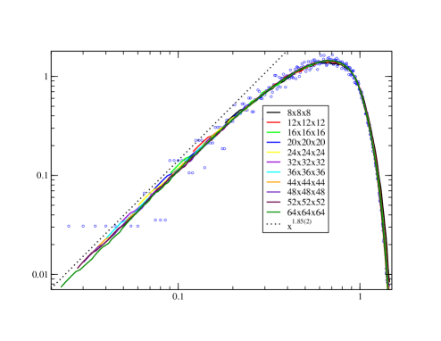
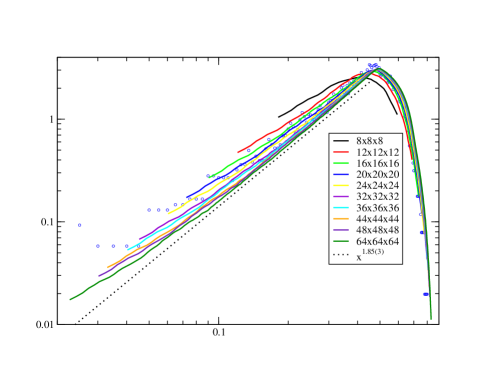
End-to-end distance. We now construct a histogram for the end-to-end distance $x_{12}=|{\bf x}_{12}|$ by summing over all possible directions of ${\bf x}_{12}$. The discrete histogram is then smoothed in a two-step process. First, for each value of $x_{12}^{(0)}$ in steps of $0.1$, we regroup the counts with $|x_{12}-x_{12}^{(0)}|<0.5$. Second, we construct a running average over 20 subsequent $x_{12}^{(0)}$ (i.e., two lattice spacings). Once properly normalized, the end result is the probability distribution (universal scaling function) of the rescaled variable $x_{\rm ee}\equiv x_{12}/L$. This is shown in Fig. 2, where (as in subsequent figures) the small circles are the $L=20$ data points after the first step of the smoothing procedure. The data collapse is strikingly good over the entire $x_{\rm ee}$ range. Before the onset of finite-size effects, we have a power law behavior

$$P(x_{\rm ee})\sim x_{\rm ee}^{1.85\pm 0.02}\mbox{ for }x_{\rm ee}\ll 1\,.$$ (1)

If the end points were independent we would have $P(x_{\rm ee})\sim x_{\rm ee}^{d-1}$ by simple geometry. The result (1) then indicates a weak effective attraction between end points.

Conformational exponents. For a HW of length $N$, the radius of gyration $R_{\rm g}\sim L$, and the exponent $\nu$ appearing in $R_{\rm g}\sim N^{\nu}$ is trivially $\nu=\frac{1}{d}=\frac{1}{3}$.

The exponent $\gamma$ describes the ratio between the number of HW ($\sim\mu^{N}N^{\gamma-1}$) and HC ($\sim\mu^{N}N^{-\nu d}$) passing through a fixed point. This leads to

$$P(x_{12}=1)\sim L^{-\gamma d}\,,\qquad\gamma=0.96\pm 0.01\,.$$ (2)

Standard scaling deGennes gives $\gamma=1-\Delta_{1}$ and $P(x_{\rm ee})\sim x_{\rm ee}^{2-2\Delta_{1}}$, and comparing (1)–(2) yields then our final estimate $\Delta_{1}=0.06\pm 0.02$.

Surface effects. We next examine the interaction of the HW with the surfaces of the system. Although globular proteins would be more realistically modeled within a spherical domain (where we expect our algorithm to be ergodic as well), we maintain here the geometry of a cube in order to have several types of surface sites.

Figure 3: Normalized probability distribution of $x_{\rm S}\equiv d_{\rm S}/L$, where $d_{\rm S}$ is the distance to the nearest side of the cube.

Figure 4: Normalized probability distribution of $x_{\rm E}\equiv d_{\rm E}/L$, where $d_{\rm E}$ is the distance to the nearest edge of the cube.

Figure 5: Normalized probability distribution of $x_{\rm C}\equiv d_{\rm C}/L$, where $d_{\rm C}$ is the distance to the nearest corner of the cube.

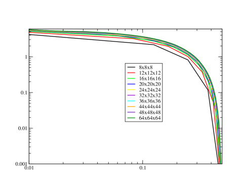
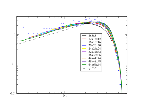
For a given end point, let $d_{\rm S}$, $d_{\rm E}$, and $d_{\rm C}$ be respectively its distance to the nearest side, edge, and corner of the cube. For each of these we construct the normalized probability distribution as above. [Since $d_{\rm S}$ is an integer, we do not apply the smoothing procedure in this case.] The results, shown in Figs. 3–5, in all cases lead to very satisfactory data collapses. Power-law fits analogous to (1) give $P(x_{\rm E})\sim x_{\rm E}^{0.72\pm 0.03}$ and $P(x_{\rm C})\sim x_{\rm C}^{1.85\pm 0.03}$; the geometric exponents for a non-interacting system would be $1$ and $2$ respectively.

The behavior of $x_{\rm S}\equiv d_{\rm S}/L$ in Fig. 3 would seem in favor of $P(x_{\rm S})\to p_{\rm S}^{0}$ as $x_{\rm S}\to 0$, with a finite value $p_{\rm S}^{0}$. However, using only the data with $d_{\rm S}=0$, we estimate $P(d_{\rm S}=0)\sim L^{-0.94\pm 0.02}$, implying that $P(x_{\rm S})\sim x_{\rm S}^{0.06\pm 0.02}$.

Figure 6: Normalized probabilities for an end point being a corner site ($p_{\rm C}$), an edge site ($p_{\rm E}$), a side site ($p_{\rm S}$), or a bulk site ($p_{\rm B}$), as functions of $1/L$.

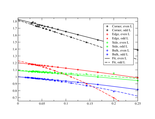
To check in more detail the affinities of the end points to the boundary, we divide the lattice sites in four classes:

$$\begin{array}[]{lll}\mbox{C:}&8\mbox{ corner sites }&\mbox{with }d_{\rm C}=0\\ \mbox{E:}&12(L-2)\mbox{ edge sites}&\mbox{with }d_{\rm E}=0,\mbox{ but }d_{\rm C}>0\\ \mbox{S:}&6(L-2)^{2}\mbox{ side sites}&\mbox{with }d_{\rm S}=0,\mbox{ but }d_{\rm E}>0\\ \mbox{B:}&(L-2)^{3}\mbox{ bulk sites}&\mbox{with }d_{\rm S}>0\\ \end{array}$$

Equivalently, the coordination number (number of links adjacent to a site) is 3 for C-sites, 4 for E-sites, 5 for S-sites, and 6 for B-sites.

We normalize the probability $p_{i}$ of an end point belonging to a given class $i={\rm C,E,S,B}$ by the ratio of $i$-type sites on the lattice. These probabilities are shown as functions of $1/L$ in Fig. 6. Note that for even (resp. odd) $L$, a HW can link any given corner site to 3 (resp. 7) other corners. Therefore, we plot $p_{\rm C}$ for even $L$ and $\frac{1}{2}p_{\rm C}$ for odd $L$. With this convention, parity effects are seen to vanish as $L\to\infty$, within error bars, and we find $p_{\rm C}=1.82\pm 0.02$, $p_{\rm E}=1.21\pm 0.01$, $p_{\rm S}=1.089\pm 0.002$, and $p_{\rm B}=1.0000\pm 0.0001$. Thus, the higher the coordination number of a site, the more do the end points tend to avoid it (in our normalization). This is remarkable, since naively one might have expected the opposite to occur.

One may similarly study the normalized probabilities $p_{ij}$ that both end points belong to prescribed classes $i$ and $j$. From this we form the matrix of cross correlations $A$ with entries $A_{ij}=\frac{p_{ij}}{p_{i}p_{j}}-1$. Note that if the two end points were statistically independent, all $A_{ij}$ would be zero. For $L=19$ we find

$$A=\left[\begin{array}[]{rrrr}-0.100&-0.020&-0.006&0.004\\ &-0.020&-0.005&0.003\\ &&-0.004&0.002\\ &&&-0.001\\ \end{array}\right]$$ (3)

Although the entries are numerically small, there is a clear qualitative effect. Namely, if one end point is at a site of small coordination number, the other end point will try to compensate by being at a site of high coordination number. In particular, it is ten percent less likely to find both end points in corners than would have been expected from the data for just one end point.

Conclusion. We have presented an algorithm that allows for efficient and unbiased sampling of three-dimensional lattice protein conformations (Hamiltonian walks). We applied it to the flexible homopolymer case, where each conformation has the same energy, and extracted a number of results on the correlation between end points and their interaction with the boundaries of the system. The most salient features are 1) the weak entropic attraction between end points, 2) the attraction of end points towards the surface, edge sites in particular, 3) their preference for sites with low coordination number, and 4) the vanishing of parity effects for $L\to\infty$.

We hope to study later topological issues, such as the knot formation probability.

It is a straightforward extension of our algorithm to associate an energy to each state and implement a standard Metropolis dynamics. This would allow to study models with bending rigidity, amino acid interactions, etc.

A slightly modified algorithm in which end points are allowed to grow or retract can be applied to models of non-compact conformations. In the standard SAW case, it decorrelates a polymer of length $N$ in time $\sim N$, not only globally (as does the pivot algorithm pivot ) but also locally. We shall report more on this elsewhere.

Acknowledgments. This work was supported through the European Community Network ENRAGE (grant MRTN-CT-2004-005616) and by the Agence Nationale de la Recherche (grant ANR-06-BLAN-0124-03).

References

- (1) P.-G. de Gennes, Scaling concepts in polymer physics (Cornell University Press, New York, 1979).
- (2) P.J. Flory, Proc. Roy. Soc. London A 234, 60 (1956).
- (3) K.A. Dill, Protein Science 8, 1166 (1999).
- (4) J.L. Jacobsen, Conformal field theory applied to loop models, in A.J. Guttmann (ed.), Polygons, polyominoes and polyhedra (Springer, in press 2007).
- (5) J.L. Jacobsen and J. Kondev, Nucl. Phys. B 532, 635 (1998); Phys. Rev. E 69, 066108 (2004).
- (6) V.S. Pande, A.Y. Grosberg, C. Joerg and T. Tanaka, J. Phys. A 27 6231 (1994).
- (7) M. Lal, Molec. Phys. 17, 57 (1969); N. Madras and A.D. Sokal, J. Stat. Phys. 50, 109 (1988); B. Li, N. Madras and A.D. Sokal, J. Stat. Phys. 80, 661 (1995).
- (8) J. Zhang, R. Chen, C. Tang and J. Liang, J. Chem. Phys. 118, 6102 (2003).
- (9) R. Oberdorf, A. Ferguson, J.L. Jacobsen and J. Kondev, Phys. Rev. E 74, 051801 (2006).
- (10) J.L. Jacobsen, preprint (2007).