Plasmons, plasminos and Landau damping in a quasiparticle model of the quark-gluon plasma

Abstract

A phenomenological quasiparticle model is surveyed for 2+1 quark flavors and compared with recent lattice QCD results. Emphasis is devoted to the effects of plasmons, plasminos and Landau damping. It is shown that thermodynamic bulk quantities, known at zero chemical potential, can uniquely be mapped towards nonzero chemical potential by means of a thermodynamic consistency condition and a stationarity condition.

1 Introduction

Intense experimental and theoretical investigations KMR03 suggest the existence of a new, deconfined phase of strongly interacting matter, where quarks and gluons form a fluid or gas, the quark-gluon plasma (QGP). If confirmed, the QGP would have existed during the Big Bang prior to hadronization and might be found inside of massive neutron stars. Indeed, recent results from the Relativistic Heavy Ion Collider (RHIC) experiments point to the formation of a quark-gluon medium of low viscosity BRA05 ; PHO05 ; STA05 ; PHE05 .

However, on the theoretical side, much work remains to be done. Perturbative solutions of QCD AZ95 ; ZK95 ; Kaj03 ; Vuo03a ; Vuo03b ; IRV04 are limited to the region of asymptotic freedom and fail for the strong coupling regime (e.g. in the vicinity of the pseudocritical temperature BI02 of deconfinement $T_{c}$; at somewhat higher temperatures, say above $2T_{c}$ resummation improves the convergence of perturbation theory noticeably KPP97 ; ABS99 ; BIR01 ). Numerical evaluations of the full theory, on the other hand, are still restricted to small chemical potential as being useful for the Big Bang or heavy-ion collisions at present RHIC top energies or future LHC energies. However, at RHIC bottom energies, at SPS energies and, in particular, at FAIR energies, baryon density effects become significant and require different approaches.

Quasiparticle models (QPM), describing the quark-gluon plasma as assembly of essentially non-interacting excitations emerging from the strong interaction, have proven to represent useful phenomenological parametrizations of QCD thermodynamics above $T_{c}$ Pes94 ; LH98 ; Pes02 ; LR03 ; TSW04 . At zero chemical potential, lattice results are described with surprising accuracy allowing the adjustment of model parameters. Thermodynamic self-consistency, supplemented by the stationarity of the thermodynamic potential, can then be used to extrapolate thermodynamic properties of systems to nonzero net baryon density.

Our quasiparticle model KBS06 ; BKS06 ; BKS07a ; BKS07b is based on the HTL approximation BP90a to the 1-loop self-energies. This gives rise to four quasiparticle families. While quasiquarks and transversal gluons within the model represent excitations with quantum numbers of actual quarks and gluons with modified masses, quark holes (plasminos) and longitudinal gluons (plasmons) are quanta of collective excitations. The residues of the poles in the spectral density of the collective modes vanish exponentially for momenta $k\sim T$, from which the main contributions to thermodynamic phase space integrals originate. Therefore, they were neglected in the previous simple form of the model (dubbed eQP in Pes05 ). Additionally, damping contributions were neglected as they are small at zero chemical potential, $\mu=0$.

The procedure of mapping the eQP results from $\mu=0$ into the $T$-$\mu$ plane is plagued by some ambiguities leading to non-unique solutions close to the presumed phase transition. Therefore, the model is restricted to sufficiently large temperatures. First attempts to include collective excitations into a two-flavor quasiparticle model at nonzero chemical potential have been made RR03 and suggest that these ambiguities might vanish. In this work we show that both collective excitations and damping effects are necessary to preserve the self-consistency of the model and ensure unique solutions when extrapolating towards large baryon densities at moderate temperatures. In the present work, the 2+1 flavor case is considered, allowing the use and extrapolation of recent lattice data Kar07 .

Our paper is organized as follows. Section 2 will comprise the derivation of the full HTL-based QPM, including collective modes and damping, as a series of approximations from QCD. The necessary further approximations leading to the eQP and its problems are discussed in section 3. The results for both models are then contrasted in section 4 and investigated in some detail. Finally, a conclusion is given in section 5.

2 Derivation of the full HTL model

2.1 The effective action

A connection of the fundamental theory of QCD and the thermodynamic potential of the QGP is provided by the Luttinger-Ward formalism LW60 ; Bay62 as shown in BKS07a . Alternatively, the Cornwall-Jackiw-Tomboulis (CJT) formalism CJT74 may be used, as a translationally invariant QGP in equilibrium and without spontaneously broken symmetries is considered. In this case, both formalisms are equivalent Ris03 .

The CJT formalism requires the stationarity of the effective action

$$\Gamma[D,S]=I -\frac{1}{2}\left\{\text{Tr}\left[\ln D^{-1}\right]+\text{Tr}\left[D_{0}^{-1}D-1\right]\right\}$$

$$+\quad\left\{\text{Tr}\left[\ln S^{-1}\right]+\text{Tr}\left[S_{0}^{-1}S-1\right]\right\}\,\,+\,\,\Gamma_{2}[D,S],$$ (1)

where $I$ is the classical action and $D$ and $S$ are the full gluon and quark propagators while the subscript $0$ denotes the respective free equivalents. The functional $\Gamma_{2}$ represents the sum over all two-particle irreducible skeleton graphs of the theory. The traces Tr contain the integration over the four-dimensional phase space as well as a trace tr over discrete indices. The integration is performed using the imaginary time formalism LeB96 ; Kap89 ; YHM95 . For the grand canonical potential $\Omega=-T\Gamma$ Bro92 ; Riv88 this yields

$$\frac{\Omega}{V} = \mbox{tr}\!\!\int\!\!\frac{\mathrm{d}^{4}k}{(2\pi)^{4}}n_{\text{B}}(\omega)\,\mbox{Im}\!\left(\ln D^{-1}-\Pi D\right)+2\,\mbox{tr}\!\!\int\!\!\frac{\mathrm{d}^{4}k}{(2\pi)^{4}}n_{\text{F}}(\omega)\,\mbox{Im}\!\left(\ln S^{-1}-\Sigma S\right)-\frac{T}{V}\Gamma_{2},$$ (2)

where $n_{\text{B}}=(\exp\,(\beta\omega)-1)^{-1}$ with $\beta=1/T$ is the Bose-Einstein, and $n_{\text{F}}=(\exp(\beta(\omega-\mu))+1)^{-1}$ the Fermi-Dirac distribution function.

2.2 Application to QCD

In our present approach, the infinite sum $\Gamma_{2}$ is truncated at 2-loop order leaving the contributions exhibited e.g. in equation (25) in BKS07a . Within the CJT formalism, the self-energies then follow from a functional derivative of $\Gamma_{2}$, giving the well-known 1-loop self-energies (e.g. equations (26) and (27) ibid.). In order to achieve a gauge invariant formulation of the model, we apply an additional approximation of hard thermal loops (HTL). Although originally being derived for soft external momenta $\omega,k\sim gT\ll T$, HTL results coincide with the complete one-loop results on the lightcone BKS07a ; Pes98b and thus provide the correct limiting behaviour.

The resulting HTL self-energies can be found in textbooks. Here we follow the conventions of Blaizot et al. BIR01 , where essential features of our model have been worked out, and use

$$\Pi_{\mu\nu} = \Pi_{\text{T}}(\omega,k)\left(\Lambda_{\text{T}}(\vec{k})\right)_{\mu\nu}-\,\,\,\,\Pi_{\text{L}}(\omega,k)\left(\Lambda_{\text{L}}(\vec{k})\right)_{\mu\nu},$$ (3)

$$\gamma_{0}\Sigma = \Sigma_{+}(\omega,k)\,\,\,\,\,\Lambda_{+}(\vec{k})\quad-\,\,\,\,\Sigma_{-}(\omega,k)\,\,\,\,\Lambda_{-}(\vec{k})$$ (4)

with the scalar self-energies

$$\Pi_{\text{T}}(\omega,k)=\frac{m_{D}^{2}}{2}\left(1+\frac{\omega^{2}-k^{2}}{k^{2}}\Pi_{\text{L}}(\omega,k)\right), \Pi_{\text{L}}(\omega,k)=m_{D}^{2}\left(1-\frac{\omega}{2k}\ln\frac{\omega+k}{\omega-k}\right),$$ (5)

$$\text{and}\quad\quad\Sigma_{\pm}(\omega,k) = \frac{\hat{M}^{2}}{k}\left(1-\frac{\omega\mp k}{2k}\ln\frac{\omega+k}{\omega-k}\right),$$ (6)

where $\hat{M}(T,\,\mu,\,g^{2})$ is the thermal fermion mass or plasma frequency and $m_{D}(T,\,\mu,\,g^{2})$ denotes the Debye screening mass

$$m_{D}^{2}=\!\left(\left[2N_{c}\!+\!N_{q}\!+\!N_{s}\right]T^{2}+\frac{N_{c}}{\pi^{2}}\sum_{i}\mu_{i}\right)\frac{g^{2}}{6} \hat{M}^{2}=\frac{N_{c}^{2}-1}{16N_{c}}\left(T^{2}+\frac{\mu^{2}}{\pi^{2}}\right)g^{2}.$$ and (7)

The number of colors $N_{c}$ is fixed at $3$. The numbers of light quarks $N_{q}=2$ and one strange quark, $N_{s}=1$, are chosen as in the lattice calculations Kar07 .

2.3 Properties of HTL self-energies and dispersion relations

The real and the imaginary parts of the HTL self-energies (5) and (6) are LeB96

$$\text{Re}\Pi_{T}=\frac{m_{D}^{2}}{2}\left(1+\frac{\omega^{2}\!-\!k^{2}}{k^{2}}\text{Re}\Pi_{\text{L}}(\omega,k)\right)\!, \text{Im}\Pi_{T}=\frac{1}{2}m_{D}^{2}\frac{\omega^{2}\!-\!k^{2}}{k^{2}}\frac{\omega}{2k}\pi\Theta\left(k^{2}\!-\!\omega^{2}\right)\varepsilon(k),$$ (8)

$$\text{Re}\Pi_{L}=m_{D}^{2}\left(1-\frac{\omega}{2k}\ln\left|\frac{\omega+k}{\omega-k}\right|\right)\!, \text{Im}\Pi_{L}=m_{D}^{2}\frac{\omega}{2k}\pi\Theta\left(k^{2}-\omega^{2}\right)\varepsilon(k),$$ (9)

$$\text{Re}\Sigma_{\pm}=\frac{\hat{M}^{2}}{k}\left(1-\frac{\omega\mp k}{2k}\ln\left|\frac{\omega+k}{\omega-k}\right|\right)\!, \text{Im}\Sigma_{\pm}=\frac{\hat{M}^{2}}{k}\frac{\omega\mp k}{2k}\pi\Theta\left(k^{2}-\omega^{2}\right)\varepsilon(k),$$ (10)

where $\varepsilon(k)$ is the sign function. The real parts are symmetric with respect to $\omega$, while the imaginary parts are antisymmetric and differ from zero only for $|\omega|<k$, i.e. below the light cone. The real and imaginary parts for $k=0.5T$ are shown in Figure 1. Analogously, the quark self-energies fulfill the parity relations $\text{Re}\Sigma_{+}(-\omega)=\text{Re}\Sigma_{-}(\omega)$ and $\text{Im}\Sigma_{+}(-\omega)=-\text{Im}\Sigma_{-}(\omega)$ as shown for $k=0.5T$ in Figure 2.

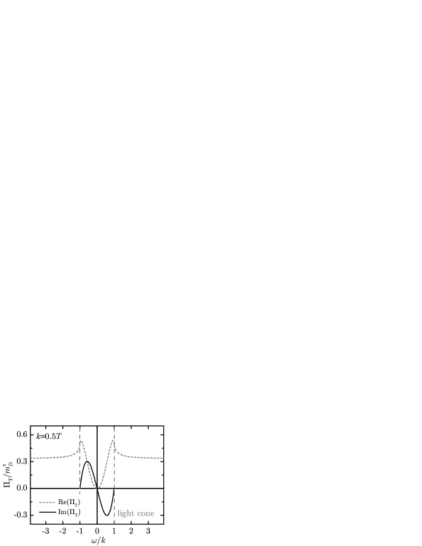
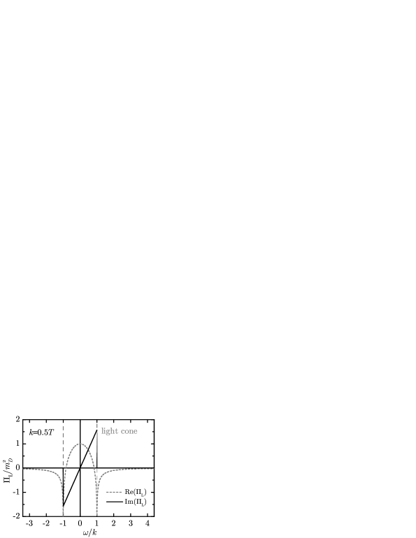
Figure 1: The real and imaginary parts of the retarded transverse (left) and longitudinal (right) gluon self-energies scaled by the Debye mass squared are shown as functions of the energy $\omega$ scaled by the momentum $k$ which is fixed at $k=0.5T$.

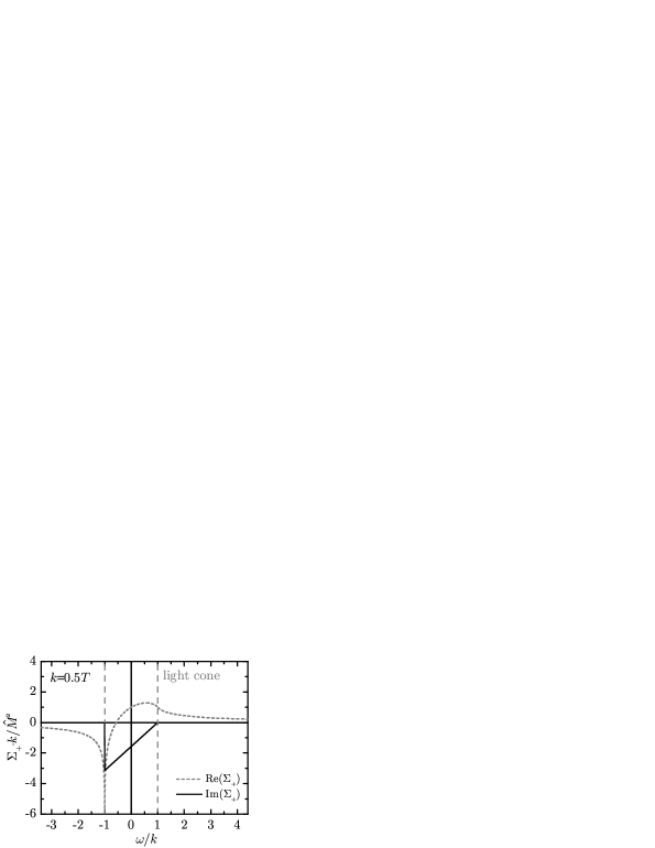
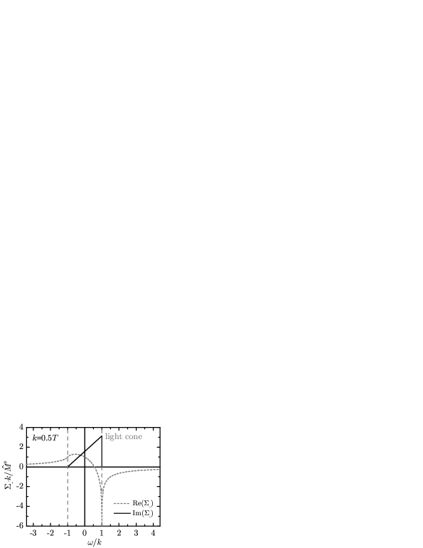
Figure 2: The real and imaginary parts of the retarded quark self-energies for the normal (left) and abnormal branch (right) scaled by the plasma frequency squared are shown as functions of the energy $\omega$ scaled by the momentum $k$ which is fixed at $k=0.5T$.

It follows directly from eqs. (8)-(10) that the HTL self-energies do not account for quasiparticle widths since the imaginary parts are zero at the poles of the quasiparticle propagators, i.e. above the light cone. The nonzero imaginary parts of the self-energies below the light cone are due to Landau damping (LD). LD is a collective effect caused by energy transfer between the gauge field and plasma particles with velocities close to the phase velocity (“resonant particles”).

Even though the imaginary parts are formally nonzero only below the light cone, retardation leads to an infinitely small contribution even above the light cone, giving a definite sign to the self-energies for all energies: $\varepsilon(\text{Im}\Pi_{\text{T}}(\omega))=-\varepsilon(\omega)$, $\varepsilon(\text{Im}\Pi_{\text{L}}(\omega))=+\varepsilon(\omega)$ and $\varepsilon(\text{Im}\Sigma_{\pm}(\omega))=\mp 1$. Note that this is not related to Landau damping which is found below the light cone only.

The HTL propagators follow from Dyson’s equations as $D_{\text{T}}^{-1}=-\omega^{2}+k^{2}+\Pi_{\text{T}}$, $D_{\text{L}}^{-1}=-k^{2}-\Pi_{\text{L}}$ and $S_{\pm}^{-1}=-\omega\pm(k+\Sigma_{\pm})$. On-shell (quasi)particles satisfy a dispersion relation determined by $\text{Re}D_{\text{T},\text{L}}^{-1}=0$ and $\text{Re}S_{\pm}^{-1}=0$ respectively. It is, therefore, useful to first investigate the real part of the inverse retarded HTL propagators.

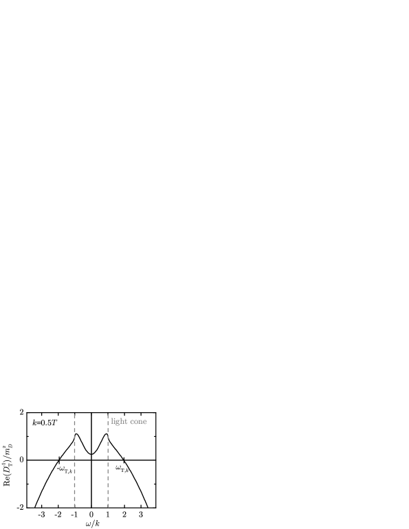
Figure 3: The real parts of the inverse gluon propagators $D_{\text{T,L}}^{-1}$ scaled by the Debye screening mass squared are shown as functions of the energy $\omega$ scaled by the momentum $k$ which is fixed at $k=0.5T$.

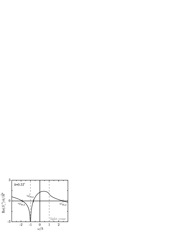
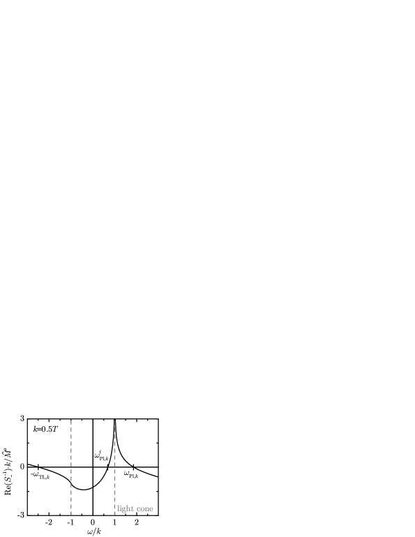
Figure 4: The real parts of the inverse quark propagators $S_{\pm}^{-1}$ scaled by the fermionic mass parameter squared are shown as functions of the energy $\omega$ scaled by the momentum $k$ which is fixed at $k=0.5T$.

Due to symmetry properties of $D_{\text{T,L}}^{-1}$ there is just one positive-energy dispersion relation above the light cone: $\omega_{\text{T},k}$ and $\omega_{\text{L},k}$, respectively. This means that - up to the sign - transverse and longitudinal gluons have the same dispersion relations as their anti(quasi)particle counterparts. The additional tachyonic dispersion relation for longitudinal gluons is related to Landau damping. Figure 3 explicitly shows the real parts for fixed momentum $k=0.5T$. Both $D_{\text{T},\text{L}}^{-1}$ are symmetric with respect to $\omega$. The zero of $\text{Re}D_{\text{T}}^{-1}$ determines the dispersion relation $\omega_{\text{T},k}$ for transverse gluons. The zero of $\text{Re}D_{\text{L}}^{-1}$ above the light cone indicates the dispersion relation $\omega_{\text{L},k}$ of longitudinal gluons, while the tachyonic dispersion relation $\omega_{\text{L},k}^{t}$ (below the light cone) is due to Landau damping.

The inverse quark propagators are not symmetric but, as a consequence of the symmetry of the self-energy, satisfy the parity property $\text{Re}S_{+}^{-1}(-\omega)=-\text{Re}S_{-}^{-1}(\omega)$ (cf. Figure 4). Hence, quarks are described by the positive energy dispersion relation related to $S_{+}$, while the dispersion relation of antiquarks is found from the negative energy solution of $\text{Re}S_{-}^{-1}=0$. The remaining two dispersion relations represent collective quark excitations: the positive energy dispersion relation related to $S_{-}$ describes the plasminos, while the negative energy solution of $\text{Re}S_{+}^{-1}=0$ represents antiplasminos. Again, a tachyonic solution appears within the regime of Landau damping.

The evolution of the zeros of the real part of the inverse retarded propagators as a function of the momentum $k$ gives the dispersion relations $\omega_{i,k}$. These dispersion relations cannot be expressed as analytic functions $\omega(k)$ in closed form. $\text{Re}D_{i}^{-1}(\omega,\,k,\,\Pi_{i}(\omega,k))=0$ and $\text{Re}S_{i}^{-1}(\omega,\,k,\,\Sigma_{i}(\omega,k))=0$ lead to transcendental equations and have to be solved numerically. The results are shown in Figures 5 and 6. Due to the above parity property quarks and antiquarks obey identical dispersion relations up to the sign, as do plasminos and antiplasminos.

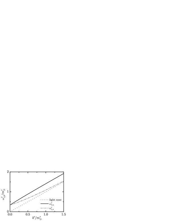
Figure 5: The dispersion relations $\omega_{\text{T},k}$ of transverse and $\omega_{\text{L},k}$ of longitudinal gluon modes scaled by the Debye screening mass are shown as functions of the momentum $k$ scaled by the Debye screening mass in linear (left) and quadratic (right) scales.

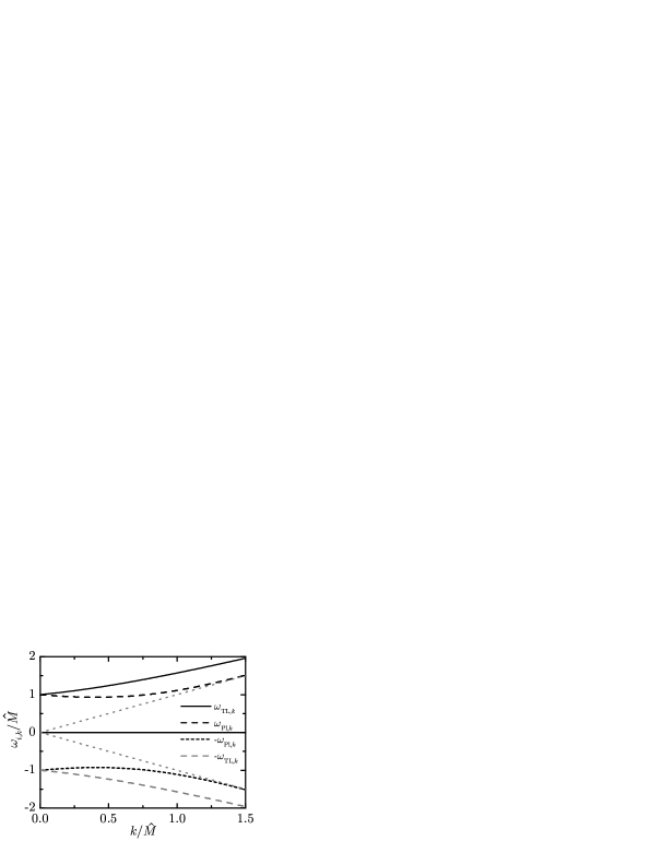
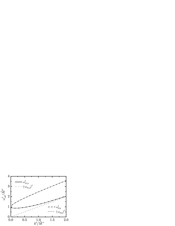
Figure 6: The dispersion relations $\omega_{i,k}$ of quarks (solid black), antiquarks (dashed grey), plasminos (black dashes) and antiplasminos (black points) scaled by the fermionic mass parameter are shown as functions of the momentum $k$ scaled by the fermionic mass parameter in linear (left) and quadratic (right) scales.

2.4 2-loop QCD entropy

Given the explicit form of the HTL self-energies and the respective propagators, we evaluate the remaining traces tr in eq. (2). Assuming equal masses for $u$ and $d$ quarks and zero chemical potential of strange quarks the isospin chemical potential $\mu_{I}=(\mu_{u}-\mu_{d})/2$ is supposed to vanish at zero net charge. Therefore, there is only one independent chemical potential $\mu=\mu_{q}=\mu_{B}/3$, where $\mu_{B}$ is the baryo-chemical potential. As a consequence the flavor trace gives equal contributions of light quarks to the thermodynamic potential (i.e. a factor $N_{q}$). The contribution of the strange quark flavor is here supposed to be equal to the light quark contribution up to a substitution of $\mu\rightarrow 0$ and $N_{q}\rightarrow N_{s}$ in the following formulae.

Taking the trace in Minkowski space, the gluonic part decomposes into three contributions for one longitudinal and two (equivalent) transverse polarizations, while the quark contribution becomes the sum of the normal and the abnormal quark branch (positive and negative chirality over helicity ratio, respectively) when taking the Dirac trace. The remaining traces only give overall factors: the color trace $(N_{c}^{2}-1)$ for the gluons and $N_{c}$ for the quarks, and the spin traces for quarks an additional $2$. Defining the prefactors $d_{g}=N_{c}^{2}-1$, $d_{q}=2N_{c}N_{q}$ and $d_{s}=2N_{c}N_{s}$ and introducing the abbreviation $\int_{\mathrm{d}^{n}k}=\int\mathrm{d}^{n}k/(2\pi)^{4}$ the HTL grand canonical potential then reads

$$\frac{\Omega}{V} = d_{g}\int_{\mathrm{d}^{4}k}\!\!n_{\text{B}}\,\Big{\{}2\text{Im}\!\left(\ln D_{\text{T}}^{-1}-D_{\text{T}}\Pi_{\text{T}}\right)+\text{Im}\!\left(\ln\left(-D_{\text{L}}^{-1}\right)+D_{\text{L}}\Pi_{\text{L}}\right)\!\Big{\}}$$

$$+2\sum_{i=q,s}d_{i}\int_{\mathrm{d}^{4}k}\!\!n_{\text{F}}\,\Big{\{}\text{Im}\!\left(\ln S_{+}^{-1}-S_{+}\Sigma_{+}\right)+\text{Im}\!\left(\ln\left(-S_{-}^{-1}\right)+S_{-}\Sigma_{-}\right)\!\Big{\}}-\frac{T}{V}\Gamma_{2}.$$

Differentiating the thermodynamic potential with respect to the temperature at constant chemical potential gives the entropy. In contrast to the pressure, which is influenced by vacuum fluctuations, the entropy is sensitive to thermal excitations and therefore manifestly ultraviolet (UV) finite. As such, it is ideally suited to investigate the properties of the QGP BIR01 .

Due to the stationarity of the thermodynamic potential with respect to the full propagators, $\delta\Omega/\delta D=0$, only the derivatives of the statistical distribution functions contribute. Using $\text{Im}(D_{\text{T}}\Pi_{\text{T}})=\text{Re}D_{\text{T}}\text{Im}\Pi_{\text{T}}+\text{Im}D_{\text{T}}\text{Re}\Pi_{\text{T}}$, the entropy density can be written as $s:=-V^{-1}\left.\partial\Omega/\partial T\right|_{\mu}=s_{g,\text{T}}+s_{g,\text{L}}+\sum_{q,s}(s_{i,+}+s_{i,-})$ with

$$s_{g,\text{T}} = -2d_{g}\int_{\mathrm{d}^{4}k}\frac{\partial n_{\text{B}}(\omega)}{\partial T}\Big{\{}\mbox{Im}\ln\left(+D_{\text{T}}^{-1}\right)-\mbox{Re}D_{\text{T}}\mbox{Im}\Pi_{\text{T}}\Big{\}},$$ (12)

$$s_{g,\text{L}} = -\,\,\,d_{g}\int_{\mathrm{d}^{4}k}\frac{\partial n_{\text{B}}(\omega)}{\partial T}\Big{\{}\mbox{Im}\ln\left(-D_{\text{L}}^{-1}\right)+\mbox{Re}D_{\text{L}}\mbox{Im}\Pi_{\text{L}}\Big{\}},$$ (13)

$$s_{q/s,\pm} = -2d_{q/s}\!\int_{\mathrm{d}^{4}k}\!\!\frac{\partial n_{\text{F}}(\omega)}{\partial T}\Big{\{}\mbox{Im}\ln\left(\pm S_{\pm}^{-1}\right)\mp\mbox{Re}S_{\pm}\mbox{Im}\Sigma_{\pm}\Big{\}},$$ (14)

each describing the entropy density of one quasiparticle species in the absence of the others. An interaction (correlation) entropy density contribution would contain terms of the form $\text{Im}D_{\text{T}}\text{Re}\Pi_{\text{T}}$ and the derivative of $\Gamma_{2}T$ with respect to the temperature. However, at 2-loop order these terms exactly cancel each other BIR01 . In fact, this seems to be a generic, topological feature CP75 which has explicitly been proven for QED VB98 and $\Phi^{4}$ theory Pes01 too.

We now focus on the terms $\text{Im}\ln(\pm D_{\text{T,L}}^{-1})$ and $\text{Im}\ln(\pm S_{\pm}^{-1})$, which can be written as

$$\text{Im}\ln D_{\text{T}}^{-1} = \arctan\left(\frac{\text{Im}D_{\text{T}}^{-1}}{\text{Re}D_{\text{T}}^{-1}}\right)+\pi\varepsilon(\text{Im}D_{\text{T}}^{-1})\Theta\!\left(-\text{Re}D_{\text{T}}^{-1}\right),$$ (15)

$$\text{Im}\ln\left(-D_{\text{L}}^{-1}\right) = \arctan\left(\frac{\text{Im}D_{\text{L}}^{-1}}{\text{Re}D_{\text{L}}^{-1}}\right)-\pi\varepsilon(\text{Im}D_{\text{L}}^{-1})\Theta\!\left(+\text{Re}D_{\text{L}}^{-1}\right).$$ (16)

Similar expressions apply for the two quark propagators: one has to substitute $S_{+}^{-1}$ for $D_{\text{T}}^{-1}$ in (15) and $S_{-}^{-1}$ for $D_{\text{L}}^{-1}$ in (16).

From the properties of the imaginary parts of the self-energies discussed above, we find $\varepsilon(\text{Im}D_{i}^{-1}(\omega))=-\varepsilon(\omega)$ for the gluons and $\varepsilon(\text{Im}S_{\pm}(\omega))\equiv-1$ for the normal and abnormal quark branches. We end up with

$$s_{g,\text{T}} = +2d_{g}\int_{\mathrm{d}^{4}k}\frac{\partial n_{\text{B}}}{\partial T}\Big{\{}\pi\varepsilon(\omega)\Theta\!\left(-\text{Re}D_{\text{T}}^{-1}\right)-\arctan\frac{\text{Im}\Pi_{\text{T}}}{\text{Re}D_{\text{T}}^{\text{-}1}}+\mbox{Re}D_{\text{T}}\mbox{Im}\Pi_{\text{T}}\Big{\}},$$ (17)

$$s_{g,\text{L}} = -\,\,\,d_{g}\int_{\mathrm{d}^{4}k}\frac{\partial n_{\text{B}}}{\partial T}\Big{\{}\pi\varepsilon(\omega)\Theta\!\left(+\text{Re}D_{\text{L}}^{-1}\right)-\arctan\frac{\text{Im}\Pi_{\text{L}}}{\text{Re}D_{\text{L}}^{\text{-}1}}+\mbox{Re}D_{\text{L}}\mbox{Im}\Pi_{\text{L}}\Big{\}},$$ (18)

$$s_{q/s,\pm} = \pm 2d_{q/s}\!\int_{\mathrm{d}^{4}k}\frac{\partial n_{\text{F}}}{\partial T}\Big{\{}\quad\,\,\,\pi\Theta\!\left(\mp\text{Re}S_{\pm}^{-1}\right)-\arctan\frac{\text{Im}\Sigma_{\pm}}{\text{Re}S_{\pm}^{\text{-}1}}\,+\mbox{Re}S_{\pm}\mbox{Im}\Sigma_{\pm}\Big{\}}.$$ (19)

The partial entropy densities (17)-(19) and, therefore the whole entropy density expression, are independent of possible renormalization factors. As required, the expression is also explicitly UV finite, as the derivatives of the distribution functions soften the UV behavior. The terms $\pi\Theta(\ldots)$ represent the quasiparticle contributions to the entropy, while the terms containing the imaginary parts of the self-energies are related to damping effects and quasiparticle widths. In the case of HTL self-energies, Landau damping is contained within the latter terms.

The quark entropy density $s_{q/s}=s_{q/s,+}+s_{q/s,-}$ can be simplified by utilizing the parity properties for quark propagators and self-energies. Introducing the distribution function of antiparticles $n_{\text{F}}^{A}=(e^{\beta(\omega+\mu)}+1)^{-1}$ with $\partial n_{\text{F}}(-\omega)/\partial\omega=-\partial n_{\text{F}}^{A}(\omega)/\partial\omega$ and substituting $\omega\rightarrow-\omega$ within $s_{q,-}$, we find

$$s_{q/s}=2d_{q/s}\int_{\mathrm{d}^{4}k}\left(\frac{\partial n_{\text{F}}}{\partial T}\!+\!\frac{\partial n_{\text{F}}^{A}}{\partial T}\right)\left\{\pi\Theta\!\left(\text{-}\text{Re}S_{+}^{-1}\right)-\arctan\!\left(\frac{\text{Im}\Sigma_{+}}{\text{Re}S_{+}^{\text{-}1}}\!\right)+\mbox{Re}S_{+}\mbox{Im}\Sigma_{+}\right\}.$$ (20)

Regarding the quasiparticle pole term $\pi\Theta(\text{-}\text{Re}S_{+}^{-1})$, the energy integration from $-\infty$ to $0$ gives the (anti)plasmino contribution, while the integration from $0$ to $+\infty$ delivers the contributions of the (anti)particles to the entropy density. Isolating both parts of the spectrum by applying the parity properties once more gives the explicit expressions

$$s_{q/s,\text{TL}} \!\!=\!\! \,\,\,\,\,2d_{q/s}\int_{\mathrm{d}^{3}k}\int\limits_{0}^{\infty}\!\frac{\mathrm{d}\omega}{2\pi}\,(.)\left\{\pi\Theta\!\left(\text{-}\text{Re}S_{+}^{-1}\right)-\arctan\!\left(\frac{\text{Im}\Sigma_{+}}{\text{Re}S_{+}^{\text{-}1}}\!\right)+\mbox{Re}S_{+}\mbox{Im}\Sigma_{+}\!\right\},$$ (21)

$$s_{q/s,\text{Pl}} \!\!=\!\! -2d_{q/s}\int_{\mathrm{d}^{3}k}\int\limits_{0}^{\infty}\!\frac{\mathrm{d}\omega}{2\pi}\,(.)\left\{\pi\Theta\!\left(\,\,\text{Re}S_{-}^{-1}\right)-\arctan\!\left(\frac{\text{Im}\Sigma_{-}}{\text{Re}S_{-}^{\text{-}1}}\!\right)+\mbox{Re}S_{-}\mbox{Im}\Sigma_{-}\!\right\},$$ (22)

where the sum of the derivatives of the distribution functions is abbreviated by the parentheses $(.)$. While this separation seems straightforward, it has to be handled with care as the Landau damping term within the quark self-energies $\Sigma_{\pm}$ (see the imaginary parts in Figure 2) can, in general, not be separated into quark and plasmino contributions in this simple way.

2.5 The full HTL QPM

Since the entropy density of the quark-gluon plasma for 2-loop QCD is the sum of the single quasiparticle entropy density contributions, it can be considered as mixture of non-interacting ideal quasiparticle gases. It is natural to assume that the pressure, which follows from the entropy density by integration, consists of single partial pressures, too. Therefore, we use the ansatz $p=p_{g,\text{T}}+p_{g,\text{L}}+\sum_{i=q,s}p_{i}-B(\Pi_{\text{T}},\Pi_{\text{L}},\Sigma_{\pm})$ for the pressure, where $B$ is chosen appropriately to ensure thermodynamic consistency. The ansatz has to satisfy $s_{i}=\partial p_{i}/\partial T|_{\mu}$ which leads to

$$p_{g,\text{T}} = +2d_{g}\int_{\mathrm{d}^{4}k}n_{\text{B}}\Big{\{}\pi\varepsilon(\omega)\Theta\!\left(-\text{Re}D_{\text{T}}^{-1}\right)-\arctan\frac{\text{Im}\Pi_{\text{T}}}{\text{Re}D_{\text{T}}^{\text{-}1}}+\mbox{Re}D_{\text{T}}\mbox{Im}\Pi_{\text{T}}\Big{\}},$$ (23)

$$p_{g,\text{L}} = -\,\,\,d_{g}\int_{\mathrm{d}^{4}k}n_{\text{B}}\Big{\{}\pi\varepsilon(\omega)\Theta\!\left(+\text{Re}D_{\text{L}}^{-1}\right)-\arctan\frac{\text{Im}\Pi_{\text{L}}}{\text{Re}D_{\text{L}}^{\text{-}1}}+\mbox{Re}D_{\text{L}}\mbox{Im}\Pi_{\text{L}}\,\Big{\}},$$ (24)

$$p_{q/\!s} = 2d_{q/\!s}\!\int_{\mathrm{d}^{4}k}\!\!\left(n_{\text{F}}\!+\!n_{\text{F}}^{A}\right)\!\Big{\{}\pi\Theta\!\left(-\text{Re}S_{+}^{-1}\right)-\arctan\frac{\text{Im}\Sigma_{+}}{\text{Re}S_{+}^{\text{-}1}}\,+\mbox{Re}S_{+}\mbox{Im}\Sigma_{+}\Big{\}},$$ (25)

where the integrability condition $\partial B/\partial\Pi_{i}=\partial p/\partial\Pi_{i}$ has to be fulfilled for every quasiparticle species $i$. Thus $B$ ensures the stationarity of the thermodynamic potential under functional variation with respect to the self-energies GY95 . Note that the plasma frequency within the $s$-quark pressure differs from the plasma frequency within $p_{q}$ as $\mu_{s}=0$.

The pressure fully defines the model. The particle density follows by differentiation of the pressure with respect to the chemical potential at constant temperature. The Bose-Einstein distribution function $n_{\text{B}}$ does not depend on $\mu_{g}$ and strange quarks are included into the model with manifest zero net particle density, therefore $n_{g,\text{T}}=n_{g,\text{L}}=n_{s}=0$ . Due to the integrability condition, the terms containing the derivatives of the self-energies with respect to $\mu$ vanish, so that

$$n\!=\!n_{q}\!\!=\!2d_{q}\!\!\int_{\mathrm{d}^{4}k}\!\!\left(\frac{\partial n_{\text{F}}}{\partial\mu}\!+\!\frac{\partial n_{\text{F}}^{A}}{\partial\mu}\right)\!\!\left\{\pi\Theta\!\left(\text{-}\text{Re}S_{+}^{-1}\right)\!-\!\arctan\frac{\text{Im}\Sigma_{+}}{\text{Re}S_{+}^{\text{-}1}}\!+\!\mbox{Re}S_{+}\mbox{Im}\Sigma_{+}\right\},$$ (26)

thus $n_{q}(\mu\rightarrow 0)\rightarrow 0$.

2.6 Effective coupling

Obviously, 2-loop QCD is only a crude approximation of the full theory. In order to accommodate non-perturbative effects in the quasiparticle model, we introduce some flexibility by parameterizing the QCD coupling constant $g^{2}$ in a phenomenologically motivated way. The truncated 2-loop running QCD coupling $g^{2}$ is given by $g^{2}(x)=16\pi^{2}(\beta_{0}\ln(x))^{-1}\,(1-2\beta_{1}\ln[\ln(x)]\,(\beta_{0}^{2}\ln(x))^{-1})$ PDG06 , where $\beta_{0}=11N_{c}/3-2N_{f}/3$, $\beta_{1}=51-19N_{f}/3$ and $N_{f}=N_{q}+N_{s}$. It depends on the ratio $x=\bar{\mu}^{2}/\Lambda^{2}$ of the renormalization scale $\bar{\mu}$ and the QCD scale parameter $\Lambda$. A term involving $\ln^{-2}(\bar{\mu}^{2}/\Lambda^{2})$ which is only a small correction for $\bar{\mu}^{2}\approx\Lambda^{2}$ was neglected.

The renormalization scale is usually taken to be the first Matsubara frequency $2\pi T$, while the latter one is just a parameter to be adjusted using experimental data. Introducing the pseudocritical temperature of QCD matter at vanishing net baryon density $T_{c}$ and substituting $\Lambda\rightarrow 2\pi T_{c}/\lambda$, the ratio $\bar{\mu}/\Lambda$ becomes $\lambda T/T_{c}$. In order to avoid the Landau pole of $g^{2}(T/T_{c})$ at $T_{c}$ a temperature shift with parameter $T_{s}$ is introduced, replacing $x$ by $\xi=\lambda(T-T_{s})/T_{c}$. The result

$$G^{2}(T\geq T_{c},\mu=0)=\frac{16\pi^{2}}{\beta_{0}\ln\xi^{2}}\left(1-\frac{2\beta_{1}}{\beta_{0}^{2}}\frac{\ln\left[\ln\xi^{2}\right]}{\ln\xi^{2}}\right)$$ (27)

is our effective coupling. Within the plasma phase for temperatures $T>T_{c}/\lambda+T_{s}$ it is well-behaved; however, at some point within the hadronic phase, i.e. below $T_{c}$, an infrared (IR) divergence does occur. In order to prevent this divergence a phenomenological infrared cutoff for $G^{2}$ can be applied. See Blu04a for details.

2.7 Adjustment to lattice calculations

The two QPM parameters $\lambda$ and $T_{s}$ have to be adjusted to results of numerical first-principle QCD calculations dubbed lattice data. Most of the past work on the QPM has been tested against lattice data from KLP00 for rather large and temperature dependent lattice restmasses of $m_{q}=0.4T$ and $m_{s}=1.0T$ compared to the physical quark masses $m_{u,d}\sim 10\,\text{M}e\text{V}$ and $m_{s}\sim 90-150\,\text{M}e\text{V}$ PDG06 . Recently, new lattice data has become available Kar07 , which relies on lattice restmasses much closer to the physical quark masses and which is used in this work.

Also, lattice calculations are performed on a finite lattice, while our quasiparticle model is formulated in the thermodynamic limit, i.e. aimed at describing a spatially infinite plasma. In order to compare our model with lattice data, the proper continuum extrapolation of the latter one is required. A safe continuum extrapolation on the lattice is a fairly demanding work. Therefore, various estimates have been applied, e.g. simply scaling the lattice results by a factor being strictly valid only for asymptotically high temperatures or for the non-interacting limit. To account for a possible deficit of such rough continuum estimates of the lattice data we introduce an ad hoc scaling factor $d_{\text{lat}}$ which turns out to be nearly unity.

2.8 Nonzero chemical potential

The parametrization of $G^{2}$ in eq. (27) is valid for $\mu=0$ only. However, it is possible to use the thermodynamic consistency of the QPM to map the results at zero chemical potential into the $T$-$\mu$ plane Pes00 . Specifically, this means to impose the Maxwell relation $\partial s/\partial\mu|_{T}=\partial n/\partial T|_{\mu}$ on the thermodynamic quantities. Ordering the terms with respect to the partial derivatives of the effective coupling gives an elliptic quasilinear partial differential equation

$$a_{T}\frac{\partial G^{2}}{\partial T}+a_{\mu}\frac{\partial G^{2}}{\partial\mu}=b,$$ (28)

named hereafter flow equation, with the coefficients $a_{T}$, $a_{\mu}$ and $b$ depending on $T$ and $\mu$ explicitly and, via the self-energies, implicitly. It is solved by the method of characteristics by introducing a curve parameter $x$, assuming that $T=T(x)$, $\mu=\mu(x)$ and $G^{2}=G^{2}(x)$. Subsequently, the comparison of $G_{,x}^{2}=G_{,T}^{2}T_{,x}+G_{,\mu}^{2}\mu_{,x}$ with the flow equation gives a system of three linear, coupled ordinary differential equations: $G_{,x}^{2}=-b$, $T_{,x}=-a_{T}$ and $\mu_{,x}=-a_{\mu}$ which can be solved using standard numerical methods. The initial condition for the flow equation is the effective coupling at $\mu=0$, with model parameters fixed by comparison of the entropy density with lattice results.

3 The effective QPM

Assuming that transversal gluons and quark particle excitations propagate predominantly on mass shells the full HTL QPM can be significantly simplified as it implies explicit (asymptotic) dispersion relations $\omega_{i}(k)$ of the form $\omega_{i}^{2}(k)=k^{2}+m_{i,\infty}^{2}$ as approximations to the full, implicit ones Pes02 . The $m_{i,\infty}$ terms depend neither on energy nor momentum and are therefore called asymptotic (thermal) masses. In order to adjust the eQP to lattice data, they can be modified to accomodate lattice restmasses $m_{i}$ using a prescription from Pis93 : $m_{i,\infty}^{2}\rightarrow m_{i}^{2}+2m_{i}m_{i,\infty}+2m_{i,\infty}^{2}$. Additionally neglecting Landau damping, i.e. assuming vanishing imaginary parts of the self-energies, and contributions from collective excitations, i.e. plasmons and (anti)plasminos, leads to the eQP. As collective excitations are exponentially suppressed and the effect of Landau damping is small at vanishing chemical potential the eQP seemed to be sufficient.

However, as previous studies of the flow equation Pes02 ; Blu04a have shown the characteristic curves emerging at $T\approx T_{c}$ cross each other in some region of finite values of $\mu$ for parameters adjusted to lattice QCD results (cf. dashed lines in Figure 8 below). This unfortunate feature prevents an unambiguous extrapolation of thermodynamic quantities into the full $T$-$\mu$-plane. Romatschke RR03 has shown for the $2$ flavor case that these crossings can be avoided by using the full HTL model. We are going to extend his line of arguing to the physically interesting case of $2+1$ flavors.

4 Investigation of the full HTL QPM

4.1 Adjustment to lattice data at $\mu=0$

While the eQP is able to accommodate arbitrary lattice restmasses by means of a modified asymptotic dispersion relation, the full HTL model relies on the HTL dispersion relations and thus massless particles. We assume here that the employed lattice restmasses in Kar07 are sufficiently small to be absorbed in suitably adjusted parameters.

For $T>T_{c}$ and $N_{f}=2$ the full HTL model has been shown to give a description of lattice data being equally well as the eQP Rom04 . For $N_{f}=2+1$ flavors we meet a similar situation: The full HTL QPM describes the lattice QCD data Kar07 as good as the eQP model (see Figure 7, left). The extension to $T<T_{c}$, on the other hand, is not straightforward. Instead of a linear IR regulator Blu04b , it is necessary to use a quadratic parametrization of the effective coupling in order to achieve agreement with lattice data also below the pseudocritical temperature, which we consider here as mere parametrisation of the lattice data.

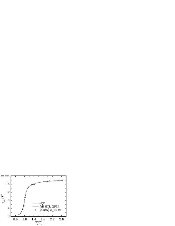
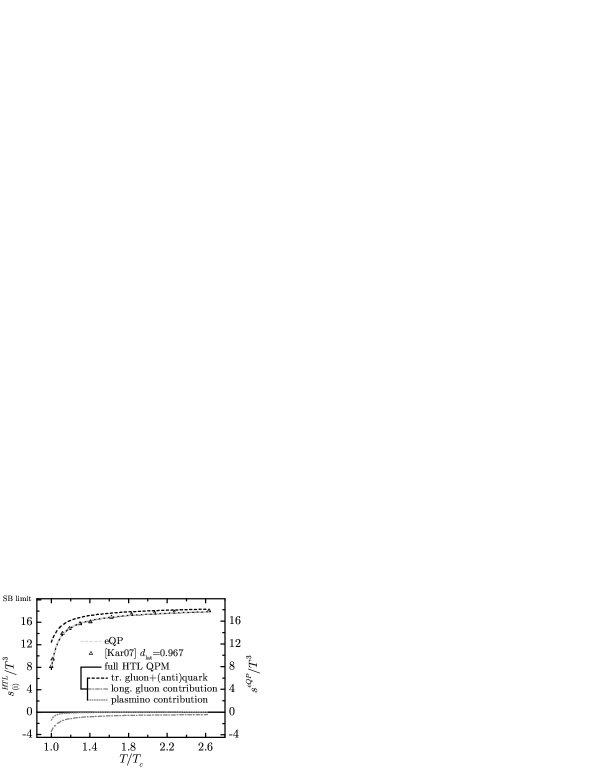
Figure 7: The scaled entropy densities $s/T^{3}$ of the full HTL QPM with quadratic IR regulator (solid black lines; $T_{s}=0.728T_{c}$ and $\lambda=6.10$) and the eQP (grey dashed lines; $T_{s}=0.752T_{c}$ and $\lambda=6.26$) adjusted to lattice data for $N_{f}=2+1$ from Kar07 with $d_{\text{lat}}=0.96$ are shown as functions of the scaled temperature $T/T_{c}$. The adjustment quality of the full HTL QPM to lattice data is indistinguishable from the eQP. The single contributions to $s^{HTL}$, including their respective LD contributions, are given in the right figure (dashed black: transversal gluons+(anti)quarks, dash-dotted: longitudinal gluons, dotted grey: (anti)plasminos).

When evaluating the individual contributions to the entropy density of the full HTL QPM we find the entropy density contributions of longitudinal gluon $s_{g,\text{L}}$ (eq. (18)) and (anti)plasminos $s_{q,\text{Pl}}$ (eq. (22)) to be negative. This is due to the fact that both represent collective phenomena of the QGP resulting in correlations not present in a noninteracting medium. As a consequence, the transverse gluon and (anti)quark entropy density contributions have to increase in comparison to the eQP in order for the sum of the partial entropy densities to describe the same lattice data as the eQP (see Figure 7, right). This not only allows for a pure quasiparticle entropy contribution much closer to the Stefan-Boltzmann limit than in the eQP but also proves to have a positive impact on the extension to nonzero chemical potential.

4.2 Solution of the flow equation

Solving the flow equation (28) with coefficients listed in Appendix A the characteristics are found to be well-behaving, as can be seen in Figure 8. Also a stronger curvature of the full HTL characteristics compared to the eQP characteristics (shown as dashed lines in the right panel) is observable.

To explain the disappearance of the ambiguities caused by crossing characteristics in the eQP we mention that the crossings appear due to the effective coupling $G^{2}$ being too large near the pseudocritical temperature Blu04 . Since the entropy density increases with decreasing mass parameters $m_{D}^{2}$ and $\hat{M}^{2}$ (which are proportional to $G^{2}T^{2}$ at $\mu=0$) the crossings would therefore disappear for a larger eQP entropy density. One way to allow for a larger eQP entropy density is to take into account collective modes. As medium effects indicate correlations between the constituents of the eQP plasma, including them causes a decrease of overall entropy density. Consequently, the eQP parameters have to change in order to still describe the same lattice data, causing the entropy density to increase. With the resulting decrease of the effective coupling $G^{2}$ the crossings partially disappear.

However, the different parametrization at $\mu=0$ alone cannot account for the complete absence of ambiguities for the full HTL model. Instead, the influence of collective modes and Landau damping on the flow equation has to be examined. We therefore calculate the characteristics of the full HTL model respectively disregarding terms stemming from these contributions. While neglecting plasmon/(anti)plasminos terms from the coefficients $a_{T}$, $a_{\mu}$ and $b$ (see Appendix A) but keeping the Landau damping contributions leads to deformed characteristics meeting $T=0$ at smaller $\mu$ and no crossings appear. Hence, it is neither the plasmon nor the plasmino term which accounts for the vanishing crossings. However, neglecting the Landau damping terms immediately leads to crossing characteristics. Therefore, both collective excitations (in order to obtain a reasonably small coupling $G^{2}$) and Landau damping (in order to ultimately remove the crossings) are necessary to obtain a flow equation with unique solutions. Using this flow equation, it is possible to extrapolate the equation of state from lattice QCD at $\mu=0$ towards $T=0$.

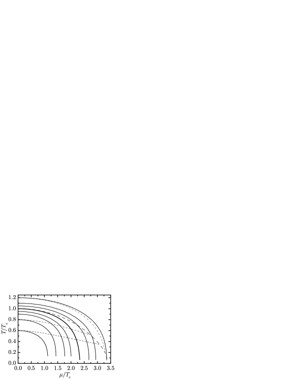
Figure 8: The solid curves in both graphs are several characteristics of the full HTL flow equation for $2+1$ quark flavors using parameters from the adjustment of the full HTL QPM to lattice data from Kar07 shown in Figure 7. The characteristic curve emerging from $T_{c}$ is depicted as bold solid line. All crossings have disappeared (left panel). For a comparison, the right panel shows the characteristics of the eQP flow equation using the parameters of the eQP adjustment to the same lattice QCD data (dashed curves).

5 Conclusion

The mapping of a previous quasiparticle model (eQP) into the $T$-$\mu$ plane was plagued by crossing characteristics. It is shown here for the 2+1 flavor case that, if using the full HTL model, these crossings disappear. Collective modes (longitudinal gluon and (anti)quark hole excitations, i.e. plasmons and (anti)plasminos respectively) as well as Landau damping of the collisionless quasiparticle plasma, both neglected hitherto in the eQP, need to be taken into account to avoid the ambiguities.

With the problem of crossing characteristics solved, one can proceed to derive an equation of state, following from the full HTL QPM, especially for the cold and dense quark-gluon plasma of interest in future heavy ion collision experiments or for the simulation of possible quark stars.

Appendix A Coefficients of the flow equation

For the reader’s convenience and to extend the results in Rom04 to $N_{f}=2+1$ flavors the full HTL flow equation is presented. To calculate the Maxwell relation, the derivatives $\partial s_{g}/\partial\mu=A_{g}\partial m_{D}^{2}/\partial\mu$, $(\partial s_{q}/\partial\mu)_{impl.}=A_{q}\partial\hat{M}^{2}/\partial\mu$, $(\partial s_{s}/\partial\mu)_{impl.}=A_{s}\partial\hat{M}^{2}/\partial\mu$ and $(\partial n_{q}/\partial T)_{impl.}=A_{n}\partial\hat{M}^{2}/\partial T$ are necessary. The explicit derivatives cancel within the Maxwell relation due to Schwarz’s Theorem. We find

$$A_{g} = \frac{d_{g}}{2\pi^{3}m_{D}^{2}}\int\limits_{0}^{\infty}\mathrm{d}k\,k^{2}\Bigg{(}\int\limits_{0}^{k}\mathrm{d}\omega\left[\frac{\partial n_{\text{B}}}{\partial T}\frac{4(\omega^{2}-k^{2})\text{Im}^{3}\Pi_{\text{T}}}{(\text{Re}^{2}D_{\text{T}}^{-1}\!+\!\text{Im}^{2}\Pi_{\text{T}})^{2}}\!-\!\frac{\partial n_{\text{B}}}{\partial T}\frac{2k^{2}\text{Im}^{3}\Pi_{\text{L}}}{(\text{Re}^{2}D_{\text{L}}^{-1}\!+\!\text{Im}^{2}\Pi_{\text{L}})^{2}}\right]$$

$$\quad\quad\quad\quad\quad\quad\quad\quad-\,\,\pi\,\frac{\omega_{\text{T},k}(\omega_{\text{T},k}^{2}-k^{2})^{2}}{|(\omega_{\text{T},k}^{2}\!-\!k^{2})^{2}\!-\!m_{D}^{2}\omega_{\text{T},k}^{2}|}\left.\frac{\partial n_{\text{B}}}{\partial T}\right|_{\omega_{\text{T},k}}\!\!\!\!\!\!\!\!-\,\pi\,\frac{\omega_{\text{L},k}(\omega_{\text{L},k}^{2}-k^{2})}{|\omega_{\text{L},k}^{2}\!-\!k^{2}\!-\!m_{D}^{2}|}\left.\frac{\partial n_{\text{B}}}{\partial T}\right|_{\omega_{\text{L},k}}\Bigg{)}$$

$$A_{q} = \frac{d_{q}}{2\pi^{3}\hat{M}^{2}}\int\limits_{0}^{\infty}\mathrm{d}k\,k^{2}\Bigg{(}\int\limits_{-k}^{k}\mathrm{d}\omega\left[{\cal N}_{T}\frac{2(\omega-k)\text{Im}^{3}\Sigma_{+}}{(\text{Re}^{2}S_{+}^{-1}\!+\!\text{Im}^{2}\Sigma_{+})^{2}}\right]$$

$$\quad\quad\quad\quad\quad\quad\quad\,\,\,\,-\pi\frac{\omega_{\text{TL},k}^{2}\!\!-k^{2}}{2\hat{M}^{2}}(\omega_{\text{TL},k}-k)\left.{\cal N}_{T}\right|_{\omega_{\text{TL},k}}-\pi\frac{\omega_{\text{Pl},k}^{2}\!\!-k^{2}}{2\hat{M}^{2}}(\omega_{\text{Pl},k}+k)\left.{\cal N}_{T}\right|_{\omega_{\text{Pl},k}}\Bigg{)}$$

$$A_{n} = \frac{d_{q}}{2\pi^{3}\hat{M}^{2}}\int\limits_{0}^{\infty}\mathrm{d}k\,k^{2}\Bigg{(}\int\limits_{-k}^{k}\mathrm{d}\omega\left[{\cal N}_{\mu}\frac{2(\omega-k)\text{Im}^{3}\Sigma_{+}}{(\text{Re}^{2}S_{+}^{-1}\!+\!\text{Im}^{2}\Sigma_{+})^{2}}\right]$$ (31)

$$\quad\quad\quad\quad\quad\quad\quad\,\,\,\,-\pi\frac{\omega_{\text{TL},k}^{2}\!\!-k^{2}}{2\hat{M}^{2}}(\omega_{\text{TL},k}-k)\left.{\cal N}_{\mu}\right|_{\omega_{\text{TL},k}}-\pi\frac{\omega_{\text{Pl},k}^{2}\!\!-k^{2}}{2\hat{M}^{2}}(\omega_{\text{Pl},k}+k)\left.{\cal N}_{\mu}\right|_{\omega_{\text{Pl},k}}\Bigg{)}$$

with abbreviations ${\cal N}_{T}:=\partial/\partial T(n_{\text{F}}+n_{\text{F}}^{A})$ and ${\cal N}_{\mu}:=\partial/\partial\mu(n_{\text{F}}+n_{\text{F}}^{A})$. The derivative of the strange quark entropy density with respect to the temperature equals the light quark expression at vanishing chemical potential with $A_{s}=A_{q}(\mu=0)$ and $\partial\hat{M}_{s}^{2}/\partial\mu=(\partial\hat{M}^{2}/\partial\mu)|_{\mu=0}$. Imposing the Maxwell relation $\partial s/\partial\mu|_{T}=\partial n/\partial T|_{\mu}$ and employing the prefactors in eq. (7) the coefficients of the flow equation (28) are given by

$$a_{T} = -\frac{N_{c}^{2}-1}{16N_{c}}\left(T^{2}+\frac{\mu^{2}}{\pi^{2}}\right)A_{n},$$ (32)

$$a_{\mu} = \frac{1}{6}\left(\left[2N_{c}+N_{q}+N_{s}\right]T^{2}+\frac{N_{c}N_{q}}{\pi^{2}}\mu^{2}\right)A_{g}$$

$$\quad\quad\quad\quad\quad\quad\,\,\,+\frac{N_{c}^{2}-1}{16N_{c}}\left(T^{2}+\frac{\mu^{2}}{\pi^{2}}\right)A_{q}+\frac{N_{c}^{2}-1}{16N_{c}}T^{2}A_{s},$$

$$b = \frac{N_{c}^{2}-1}{8N_{c}}TG^{2}A_{n}-\frac{N_{c}N_{q}}{3\pi^{2}}\mu\,G^{2}A_{g}-\frac{N_{c}^{2}-1}{8N_{c}\pi^{2}}\mu\,G^{2}A_{q}.$$ (34)

These expressions correct a few typos in Rom04 (see eqs. (B.1)-(B.5) therein).

References

- (1) J. Kapusta, B. Müller, J. Rafelski, Quark-Gluon Plasma: Theoretical Foundations (Elsevier, 2003), ISBN 0444511105
- (2) I. Arsene et al. (BRAHMS), Nucl. Phys. A 757, 1 (2005), nucl-ex/0410020
- (3) B.B. Back et al. (PHOBOS), Nucl. Phys. A 757, 28 (2005), nucl-ex/0410022
- (4) J. Adams et al. (STAR), Nucl. Phys. A 757, 102 (2005), nucl-ex/0501009
- (5) K. Adcox et al. (PHENIX), Nucl. Phys. A 757, 184 (2005), nucl-ex/0410003
- (6) P. Arnold, C. Zhai, Phys. Rev. D 51(4), 1906 (1995), hep-ph/9410360
- (7) C. Zhai, B. Kastening, Phys. Rev. D 52(12), 7232 (1995), hep-ph/9507380
- (8) K. Kajantie, M. Laine, K. Rummukainen, Y. Schröder, Phys. Rev. D 67(10), 105008 (2003), hep-ph/0211321
- (9) A. Vuorinen, Phys. Rev. D 67(7), 074032 (2003), hep-ph/0212283
- (10) A. Vuorinen, Phys. Rev. D 68(5), 054017 (2003), hep-ph/0305183
- (11) A. Ipp, A. Rebhan, A. Vuorinen, Phys. Rev. D 69(7), 077901 (2004), hep-ph/0311200
- (12) J.P. Blaizot, E. Iancu, QCD Perspectives on Hot and Dense Matter (Springer, 2002)
- (13) F. Karsch, A. Patkos, P. Petreczky, Phys. Lett. B 401, 69 (1997), hep-ph/9702376
- (14) J.O. Andersen, E. Braaten, M. Strickland, Phys. Rev. D 61(1), 014017 (1999), hep-ph/9902327
- (15) J.P. Blaizot, E. Iancu, A. Rebhan, Phys. Rev. D 63(6), 065003 (2001), hep-ph/0005003
- (16) A. Peshier, B. Kämpfer, O.P. Pavlenko, G. Soff, Phys. Lett. B 337, 235 (1994)
- (17) P. Lévai, U. Heinz, Phys. Rev. C 57(4), 1879 (1998), hep-ph/9710463
- (18) A. Peshier, B. Kämpfer, G. Soff, Phys. Rev. D 66(9), 094003 (2002), hep-ph/0206229
- (19) J. Letessier, J. Rafelski, Phys. Rev. C 67(3), 031902 (2003), hep-ph/0301099
- (20) M.A. Thaler, R.A. Schneider, W. Weise, Phys. Rev. C 69(3), 035210 (2004), hep-ph/0310251
- (21) B. Kämpfer, M. Bluhm, R. Schulze, D. Seipt, U. Heinz, Nucl. Phys. A 774, 757 (2006), hep-ph/0509146
- (22) M. Bluhm, B. Kämpfer, R. Schulze, D. Seipt, Acta Phys. Hung. A 27, 397 (2006), hep-ph/0608052
- (23) M. Bluhm, B. Kämpfer, R. Schulze, D. Seipt, Eur. Phys. J. C 49, 205 (2007), hep-ph/0608053
- (24) M. Bluhm, B. Kämpfer, R. Schulze, D. Seipt, U. Heinz, Phys. Rev. C 76, 034901 (2007), hep-ph/0705.0397
- (25) E. Braaten, R.D. Pisarski, Phys. Rev. Lett. 64(12), 1338 (1990)
- (26) A. Peshier, J. Phys. G 31(4), 371 (2005), hep-ph/0409270
- (27) A. Rebhan, P. Romatschke, Phys. Rev. D 68(2), 025022 (2003), hep-ph/0304294
- (28) F. Karsch (2007), hep-ph/0701210
- (29) J.M. Luttinger, J.C. Ward, Phys. Rev. 118(5), 1417 (1960)
- (30) G. Baym, Phys. Rev. 127(4), 1391 (1962)
- (31) J.M. Cornwall, R. Jackiw, E. Tomboulis, Phys. Rev. D 10(8), 2428 (1974)
- (32) D.H. Rischke, Prog. Part. Nucl. Phys. 52, 197 (2004), nucl-th/0305030
- (33) M.L. Bellac, Thermal Field Theory (Cambridge University Press, 1996), ISBN 0521654777
- (34) J.I. Kapusta, Finite-Temperature Field Theory (Cambridge University Press, 1989)
- (35) K. Yagi, T. Hatsuda, Y. Miake, Finite-Temperature Field Theory (Cambridge University Press, 2005), ISBN 0521561086
- (36) L.S. Brown, Quantum Field Theory (Cambridge University Press, 1992), ISBN 0521469465
- (37) R.J. Rivers, Path integral methods in quantum field theory, 1st edn. (Cambridge University Press, 1988), ISBN 0521368707
- (38) A. Peshier, K. Schertler, M.H. Thoma, Ann. Phys. 266, 162 (1998), hep-ph/9708434, http://dx.doi.org/10.1006/aphy.1997.5781
- (39) G.M. Carneiro, C.J. Pethick, Phys. Rev. B 11(3), 1106 (1975)
- (40) B. Vanderheyden, G. Baym, J. Stat. Phys. 93(3), 843 (1998)
- (41) A. Peshier, Phys. Rev. D 63(10), 105004 (2001), hep-ph/0011250
- (42) M.I. Gorenstein, S.N. Yang, Phys. Rev. D 52(9), 5206 (1995)
- (43) W.M. Yao et al. (PDG), J. Phys. G 33, 1 (2006), http://pdg.lbl.gov
- (44) M. Bluhm, B. Kämpfer, G. Soff (2004), hep-ph/0402252
- (45) F. Karsch, E. Laermann, A. Peikert, Phys. Lett. B 478, 447 (2000), hep-lat/0002003
- (46) A. Peshier, B. Kämpfer, G. Soff, Phys. Rev. C 61(4), 045203 (2000), hep-ph/9911474
- (47) R.D. Pisarski, Phys. Rev. D 47(12), 5589 (1993)
- (48) P. Romatschke, Ph.D. thesis, Technical University Vienna (2004), hep-ph/0312152
- (49) M. Bluhm, B. Kämpfer, G. Soff, Phys. Lett. B 620, 131 (2005), hep-ph/0411106
- (50) M. Bluhm, Master’s thesis, Technical University Dresden (2004)