Rate determining factors in protein model structures

Abstract

Previous research has shown a strong correlation of protein folding rates to the native state geometry, yet a complete explanation for this dependence is still lacking. Here we study the rate-geometry relationship with a simple statistical physics model, and focus on two classes of model geometries, representing ideal parallel and antiparallel structures. We find that the logarithm of the rate shows an almost perfect linear correlation with the ”absolute contact order”, but the slope depends on the particular class considered. We discuss these findings in the light of experimental results.

In the last decade many results have been published on the relationship between kinetic and structural features of protein folding, after the seminal work by Plaxco, Simons and Baker Plaxco revealed a simple linear relationship between the logarithm of the folding rate and the relative contact order (CO) for a set of two-state proteins. CO is defined as the sum of the sequence distances $|j-i|$ of any residue pair $(i,j)$ in contact in the native structure (with a ”contact” being defined according to a cutoff distance), divided by the total number of contacts and number of residues. A similar good correlation was obtained by Jackson Jackson , considering the absolute contact order (ACO, equal to CO times the number of residues) and using a slightly extended protein set. Galzitskaya et al. in GalFinkProt2003 showed that length, rather than CO, is relevant in three-state proteins. The role of the length is also considered in Thir95 ; Cieplak ; Thir2004 ; MunozJACS , while the logarithm of the relative contact order, together with CO and ACO, was considered in Grantcharova , and a combination of CO and length in Koga . The rates have been also related to linear combinations of the length and its logarithm Makarov , long range order (LRO), total contact distance Zhou , fraction of short range contacts Miller , cliquishness Micheletti , effective contact order Dixit . Plotkin and coworkers Plotkin discussed the correlation with heterogeneities in contact distance and energy, while the absolute contact order, and its length dependence, was reconsidered in Ivankov . On the basis of the cited (and certainly not exhaustive) set of investigations it is difficult to reach a definite conclusion about which measures of native state properties are most relevant to determine the folding rate. Indeed, while experimental rates show a clear correlation with the structural parameters proposed in the above literature, they are always distributed with a relevant spread around the theoretical curve, that remains to be accounted for. On- and off-lattice theoretical modelling jewpandeplaxco2003 ; kayachan2003 suggest that adding cooperativity and/or local preferential conformations to Gō like models improves the correlation of the rates with CO, also inducing spread in the rate distribution. But also the high heterogeneity of the distribution of the sequence-distance of the contacts in protein structures could be responsible for the rate spread Plotkin . For the above reasons, it is very important to try to address this issue with model structures, in the framework of a simple model with few parameters. We focus on two classes of structures, the ideal analogues of real parallel and antiparallel secondary structures ($\alpha$–helices and $\beta$–sheets): our aim is to find a set of rules that may be later used to rationalize the relationship between real protein geometries and rates.

We resort to the Wako–Saitô–Muñoz–Eaton (WSME) model, which allows an exact solution for the equilibrium thermodynamics and a very accurate semi–analytical approach to the kinetics. At difference with other native-centric models, WSME is intrinsically cooperative and accounts for the local preferences of the main-chain. The model has already been shown to give good results in the determination of rates of real proteins ME3 ; HenryEaton , their temperature dependence ZP-PRL , the effect of mutations ZP-Prep and mechanical unfolding rates IPZ . The WSME model was introduced in the end of the ’70s WS1 ; WS2 and then forgotten for roughly 20 years, when it was indepentently reproposed by Muñoz, Eaton and coworkers ME1 ; ME2 ; ME3 ; HenryEaton . Several studies followed Amos1 ; Amos2 ; ItohSasai1 ; ItohSasai2 ; ItohSasai3 ; AbeWako ; BP ; P ; ZP-PRL ; ZP-JSTAT ; IPZ also with applications in a very different subfield of physics TD1 ; TD2 ; TD3 . WSME is a Gō–like model Go , i.e. it is ”native-centric”, relying on the knowledge of the native state of a protein to describe its equilibrium and kinetics. Its binary degrees of freedom are related to the values of the dihedral angles at the peptide bonds ME2 , classified into just two states: ordered (native) and disordered (unfolded). Since the latter state allows a much larger number of microscopic realizations than the former, an entropic cost is given to the ordering of a peptide bond.

The model is described by the effective free energy:

$$H=\sum_{i=1}^{N-1}\sum_{j=i+1}^{N}\epsilon_{i,j}\Delta_{i,j}\prod_{k=i}^{j}m_{k}-RT\sum_{k=1}^{N}q_{k}(1-m_{k}),$$ (1)

where $N$ is the number of peptide bonds in the molecule, $R$ the ideal gas constant and $T$ the absolute temperature. $m_{k}\in\{0,1\}$ is the binary variable which tells whether the $k$–th bond, i.e. the one between residues $k$ and $k+1$, is in the disordered (0) or ordered (1) state, and $q_{k}$ is the corresponding ordering entropic cost. The product ${\prod_{k=i}^{j}}m_{k}$ takes value 1 if and only if all the peptide bonds from $i$ to $j$ are in the native state, thereby realizing the assumed interaction. The contact matrix with elements $\Delta_{i,j}\in\{0,1\}$ tells which peptide bonds are at close distance in the native state; non–native interactions are disregarded. The contact map beween peptide bonds, $\Delta_{i,j}$ is derived from the standard one between residues, $\Delta_{i,j}^{r}$, as $\Delta_{i,j}=\Delta_{i,j+1}^{r}$, thus assigning the (residue $i$)-(residue $j$) contact to peptide bonds $i$ and $(j-1)$. $\Delta_{i,j}^{r}$ is usually calculated according to some cutoff distance residues $i$ and $j$ in the native state; here we deal with ideal secondary structures, and will impose $\Delta_{i,j}^{r}$ accordingly. Contact energy will be taken as $\epsilon_{i,j}=-\epsilon$ throughout the paper, unless differently stated. Without loss of generality, we can set $\epsilon=1$. Also the entropic costs will be taken to be homogeneous, $q_{k}=q=2\ln 2$. Several values of these entropies have been considered in various works up to now, typically based on some fits to experimental data. Here we want to consider model structures, so the specific value is not too relevant: we take $q=2\ln 2$, comparable to the results obtained for various molecules; in the following we will discuss the $q$-dependence of our results. Notice that, once fixed $\epsilon$ and $q$, the only source of heterogeneity comes from the contact matrix, i.e., from the geometry of the native state.

We define the denaturation temperature $T_{m}$ asking that the average fraction $m$ of ordered bonds is halfway between its values $m_{0}=1$ (at T=0) and $m_{\infty}=\frac{1}{N}\sum_{k=1}^{N}(1+e^{q_{k}})^{-1}$ at infinite temperature. In the following, for each structure considered, we will always work at the corresponding $T_{m}$. Exact evaluation WS1 ; WS2 of thermodynamic quantities will be performed as in BP ; P .

The kinetic evolution of the model is described through a discrete–time master equation, $p_{t+1}(m)=\sum_{m^{\prime}}W(m^{\prime}\to m)p_{t}(m)$, for the probability distribution $p_{t}(m)$ at time $t$, where $m=\{m_{k},\,k=1,\ldots N\}$ denotes the state of the system. The transition matrix $W$ is specified by a single bond flip Metropolis rule, as in ZP-PRL ; ZP-JSTAT . The kinetics will be studied by means of the local equilibrium approach ZP-PRL ; ZP-JSTAT , where the equilibration rate $k$ can be computed as the largest eigenvalue of a matrix of rank $N(N+1)/2$. It has been shown in ZP-PRL ; ZP-JSTAT that this approach turns out to be very accurate when compared to exact or Monte Carlo results, and the rate so obtained is an upper bound of the exact one. Notably, this approach allows us to evaluate directly relaxation rates, which are the experimentally accessible quantities (at difference with folding and unfolding rates), without choosing a reaction coordinate.

We apply the model first to parallel structures (see Supplementary Material, Fig. 1), where the sequence distance of any interacting pair of residues is constant. This class includes $\alpha$–helices and parallel $\beta$–sheets. The first structural indicator we consider is the ACO, defined as

$${\rm ACO}=N_{c}^{-1}\displaystyle{\sum_{1\leq i<j\leq N}}\Delta_{i,j}(j-i+1),$$ (2)

where $N_{c}=\sum_{1\leq i<j\leq N}\Delta_{i,j}$ is the total number of contacts, and we add 1 to the usual $j-i$, since our contact matrix is defined with reference to peptide bonds, and the number of the latter involved in a contact is the corresponding number of residues minus one.

In Fig. 1 we report the natural logarithm of the equilibration rate at $T_{m}$ for several parallel structures, defined as parallel $\beta$–sheets with $s$ strands and $r$ residues per strand, where consecutive strands are separated by loops of $l$ residues not involved in any contact. In such a structure the number of peptide bonds is $N=s(r+l)-l-1$ and ACO $=r+l$; contact matrix elements are $\Delta_{i,j}=1$ if $j=i+l+r-1$ and $\Delta_{i,j}=0$ otherwise. The $\alpha$–helix corresponds to the case $l=0$, ACO $=r=4$. For every $(s,r)$ pair we consider values of $l$ from 0 up to 8 in order to vary the ACO. The effect of dilution is also considered (for $s=4$, $r=6$ only), where this regular structure is perturbed by removing contacts with probability $1-p$. The value of $p$, when not otherwise specified, is 1.

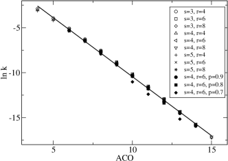
Figure 1: Logarithm of equilibration rate vs. absolute contact order for parallel structures. Symbols explained in text.

We see that all the results fall almost perfectly on the same straight line. A joint linear fit including all data yields $\ln k=2.6633-1.3113$ ACO, with correlation coefficient -0.998. Considering different values for the entropic costs would not change the overall behaviour but only the slope. For instance, $q=2$ yields a slope -1.73.

This result means that, according to this model, the ACO is of fundamental importance, while the rate cannot depend in a relevant way on other measures like the CO or the chain length, since each ACO value corresponds to several values of CO and total length. LRO, total contact distance, the fraction of short range contacts, and heterogeneity in contact distance are not applicable here, since all contacts present the same sequence distance. Even the introduction of contact-energy heterogeneities does not affects the rate: considering $s=4$, $r=7$ and $l=0$ and 4, and taking $\epsilon_{i,j}$ uniformly distributed in $[-\epsilon-\Delta\epsilon,-\epsilon+\Delta\epsilon]$, with $\Delta\epsilon\in[0,\epsilon]$, we found that the variation of $\ln k$ was compatible with the spread in Fig. 1: less than 0.02 in absolute value for $l=0$ ($\ln k\simeq-5.45$ in the uniform case), and less than 0.6 for $l=4$ ($\ln k\simeq-10.39$ in the uniform case). These figures hardly change if we consider the interactions as product of charges associated to residues, as in Tiana2004 , and take random charges, or if we consider a correlated disorder, e.g. strenghtening the contacts of a group of three consecutive residues, leaving the others unchanged. In view of the above result it is worth checking whether this almost perfect linear behaviour still holds for structures which maintain some regularity, but where the contact distance is not constant. We therefore turn to antiparallel structures, and extend the results reported in ZP-PRL for a four–stranded antiparallel $\beta$–sheet, considering sheets with $s$ strands and $r$ residues per strand; in the case $s=2$ we have a simple hairpin (see Supplementary Material, Fig. 2). Turns corresponds to peptide bonds $kr$; contacts are established between bonds $i$ and $j=2kr-i$, with $(k-1)r+1\leq i\leq kr-1$ and $k=1,\cdots,s-1$ labelling the turns; the total number of peptide bonds is $N=sr-1$. This represents the most connected case: every residue but two (in the first and last turn) has at least one contact. The contact distance varies from 3 to $2r-1$ in steps of 2, and hence ACO $=r+1$.

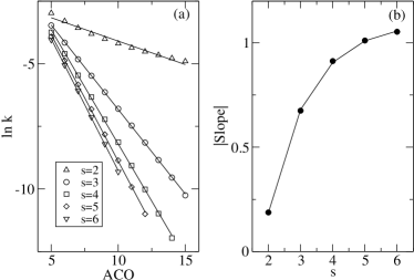
Figure 2: (a) Logarithm of equilibration rate vs. absolute contact order for antiparallel structures at the denaturation temperature $T_{m}$. Symbols explained in text. (b) Absolute value of the slope in (a) as a function of $s$.

In Fig. 2(a) we report the natural logarithm of the equilibration rate at $T_{m}$ as a function of ACO for several $(s,r)$ values. It is clearly seen that the almost perfect linear correlation is now valid only at fixed strand number $s$ (again, slopes would be larger for a larger entropic cost $q$). The absolute value of the slope increases with $s$ and appears to tend to a constant for large $s$. Indeed, a fit to an exponential function is made in panel (b) and is almost perfect ($|{\rm Slope}|=1.21-3.5\exp(-0.62s)$, estimated variance is 0.00017, correlation coefficient is 0.9996).

The limiting value of the slope is slightly smaller than that obtained for parallel structures, whence we have that, at fixed ACO$\gtrsim 4$, the hairpin is the fastest structure, then the other antiparallel structures come, in order of increasing $s$, and finally we have the parallel structures.

The exponential dependence of the logarithm of the rate on $s$ is quite puzzling: to understand such a behavior, we study the folding mechanism, as revealed by the probabilities of native ”strings” $S_{i,j}$, i.e., of configurations where peptide bonds $i$ and $j$ are unfolded, while all those in between them are native. Assuming that the relaxation rate can be related to the height of the highest barrier along the folding pathway, the analysis reveals that the latter is represented by the folding of one hairpin, or more precisely of all the residues between peptide bond $u=(k-1)r$ and $v=(k+1)r+1$, being $u$ and $v$ unfolded, for any $k$ between 1 and $(s-1)$. The probability of such a configuration can be estimated as $p(S_{u,v})=\exp(\beta_{m}\epsilon(r-1)-2rq)/Z_{u,v}$, where $\beta_{m}=1/(RT_{m})$. $Z_{u,v}$ is the partition function restricted to the region between $u$ and $v$. It can be estimated as

$$Z_{u,v} = A^{2r-1}+Ae^{\beta_{m}\epsilon(r-1)-(2r-1)q}$$ (3)

$$+ (2e^{-q}+1)\sum_{j=0}^{r-2}A^{2(r-j)-3}e^{\beta_{m}\epsilon j-(2j+1)q},$$

where $A=(1+\exp(-q))$. If our system can be considered a two-state folder we have that the relaxation rate $k=k_{f}+k_{u}$ is the sum of the folding and unfolding rates; the latter will be identical at $T=T_{m}$ and, assuming an Arrhenius scheme, they will be proportional to the folding probability $p(S_{u,v})$. So, if the above assumptions hold and we have identified the correct barrier, we will find the same behavior for $\ln p(S_{u,v})$ as for $\ln k$. Notice that the expression of $p(S_{u,v})$ contains clearly the ACO, since $r$=ACO-1, while the only quantity depending on $s$ is the value of $\beta_{m}$: one finds indeed that the exponential dependence of $\ln k$ on $s$ is related to the dependence of $\beta_{m}$ on s and ACO. Taking this into account in the expression of $p(S_{u,v})$ yields a dependence on ACO which is completely analogous to that reported in Fig.  2, where again $\ln p(S_{u,v})$ can be fitted by straight lines whose slopes follow the law: $|{\rm Slope}|=1.40-5.1\exp(-0.70s)$, (estimated variance: 0.0012, correlation coefficient: 0.9980) reasonably close to the value obtained for the rates.

The above result is very interesting, because it proves that an Arrhenius framework can still be applied in this case, despite the free-energy profiles may present more than one minimum and barrier. But even more, these results establish a quantitative connection between the rate and the number of strands through the stability, stating that as the number of strands of the system increases, the $T_{m}$ increases asymptotically, implying a global increase of the stability, while the equilibration rate decreases. Notice that the dependence of the rate on $s$ found in the model is consistent with the reported observation of a $L^{\alpha}$ - dependence Ivankov : indeed if we fit the rate to the number of residues $L=sr$ we find for the antiparallel structures $\ln k=-0.73\times L^{0.64}$, which is not far from the experimental exponent reported in Ivankov ($\alpha=0.70$) and from $\alpha=0.61$ coming from off-lattice simulations Koga . However, an accurate comparison of the dependence of rates on length should take into account the frequency of the different structures in real proteins, which is out of the scope of the present work.

To conclude, let us review the main findings: resorting to a simple statistical model, we have performed a detailed analysis of the dependence of the relaxation rate on some structural indicators, known to correlate with protein folding times. To elucidate the role and the interplay of the different factors, we have studied ideal helical, parallel and antiparallel secondary structures, of different length and number of strands. Our results confirm the absolute contact order ACO as the main structural determinant of the rates, but suggest different folding mechanisms for parallel and antiparallel structures: the latter, which fold faster than the former at equal ACO, show a dependence on the number of strands which we can relate to the dependence of the denaturation temperature on the ACO and number of strands. We also find that the dependence of the rate on the length of the protein is consistent with the power-law reported in Ivankov for real proteins, despite the fact our ideal structures lack the structural and energetic heterogeneity of the latter.

P. B. acknowledges support from Spanish Education and Science Ministry (FIS2004-05073, FIS2006-12781).

References

- (1) K. W. Plaxco, K. T. Simons and D. Baker, J. Mol. Biol. 277, 985 (1998).
- (2) S. E. Jackson, Fold. Des. 3, R81 (1998).
- (3) O. V. Galzitskaya,S. O. Garbuzynskiy, D. N. Ivankov, and A. V. Finkelstein, Proteins: Struct. Funct. Genet. 51, 162 (2003).
- (4) D. Thirumalai, J. Phys. I (France) 5, 1457 (1995).
- (5) M. Cieplak and T.X. Hoang, Biophys. J. 84, 475 (2003).
- (6) M. S. Li, D. K. Klimov, andD. Thirumalai, Polymer 45, 573 (2004).
- (7) A. N. Naganathan and V. Muñoz, J. Am. Chem. Soc. 127, 480 (2005).
- (8) V. Grantcharova, E. J. Alm, D. Baker and A. L. Horwich, Curr. Opin. Struct. Biol. 11, 70 (2001).
- (9) N. Koga and S. Takada, J. Mol. Biol. 313, 171 (2001).
- (10) D.E. Makarov, C.A. Keller, K.W. Plaxco and H. Metiu, Proc. Natl. Acad. Sci. U.S.A. 99, 3535 (2002).
- (11) H. Zhou and Y. Zhou, Biophys. J. 82, 458 (2002).
- (12) E.J. Miller, K.F. Fischer and S. Marqusee, Proc. Natl. Acad. Sci. U.S.A. 99, 10359 (2002).
- (13) C. Micheletti, Proteins: Struct. Funct. Genet. 51, 74 (2003).
- (14) P.D. Dixit and T.R. Weikl, Proteins: Struct. Funct. Bioinf. 64, 193 (2006).
- (15) B. Ötzop, M.R. Ejtehadi and S.S. Plotkin, Phys. Rev. Lett. 93, 208105 (2004).
- (16) D. N. Ivankov, S. O. Garbuzynskiy, E. Alm, K. W. Plaxco,D. Baker, and A. V. Finkelstein, Protein Sci. 12, 2057 (2003).
- (17) A. I. Jewett,V. S. Pande, and K. W. Plaxco, J. Mol. Biol. 326, 247 (2003).
- (18) H. Kaya and H. S. Chan, Proteins: Struct. Funct. Genet.,52, 524 (2003).
- (19) V. Muñoz and W.A. Eaton, Proc. Natl. Acad. Sci. U.S.A. 96, 11311 (1999).
- (20) E.R. Henry, W.A. Eaton, Chem. Phys. 307, 163 (2004).
- (21) M. Zamparo and A. Pelizzola, Phys. Rev. Lett. 97, 068106 (2006).
- (22) A. Pelizzola and M. Zamparo, in preparation.
- (23) A. Imparato, A. Pelizzola and M. Zamparo, Phys. Rev. Lett. 98, 148102 (2007).
- (24) H. Wako and N. Saitô, J. Phys. Soc. Jpn 44, 1931 (1978).
- (25) H. Wako and N. Saitô, J. Phys. Soc. Jpn 44, 1939 (1978).
- (26) V. Muñoz, P.A. Thompson, J. Hofrichter and W.A. Eaton, Nature 390, 196 (1997).
- (27) V. Muñoz, E.R. Henry, J. Hofrichter and W.A. Eaton, Proc. Natl. Acad. Sci. U.S.A. 95, 5872 (1998).
- (28) A. Flammini, J.R. Banavar and A. Maritan, Europhys. Lett. 58, 623 (2002).
- (29) I. Chang, M. Cieplak, J.R. Banavar and A. Maritan, Protein Sci. 13, 2446 (2004).
- (30) K. Itoh and M. Sasai, Proc. Natl. Acad. Sci. U.S.A. 101, 14736 (2004).
- (31) K. Itoh and M. Sasai, Chem. Phys. 307, 121 (2004).
- (32) K. Itoh and M. Sasai, Proc. Natl. Acad. Sci. U.S.A. 103, 7298 (2006).
- (33) H. Abe and H. Wako, Phys. Rev. E 74, 011913 (2006).
- (34) P. Bruscolini and A. Pelizzola, Phys. Rev. Lett. 88, 258101 (2002).
- (35) A. Pelizzola, J. Stat. Mech., P11010 (2005).
- (36) M. Zamparo and A. Pelizzola, J. Stat. Mech., P12009 (2006).
- (37) V. I. Tokar and H. Dreyssé, Phys. Rev. E 68, 011601 (2003).
- (38) V. I. Tokar and H. Dreyssé, J. Phys. Cond. Matter 16, S2203 (2004).
- (39) V. I. Tokar and H. Dreyssé, Phys. Rev. E 71, 031604 (2005).
- (40) Y. Udea, H. Taketomi, N. Gō, Biopolymers 17, 1531 (1978).
- (41) G. Tiana, F. Simona, G. M. S. De Mori, R. A. Broglia and G. Colombo, Prot. Sci. 13, 113 (2004).