Hard X-ray Variability of AGN

Abstract

Aims. Active Galactic Nuclei are known to be variable throughout the electromagnetic spectrum. An energy domain poorly studied in this respect is the hard X-ray range above 20 keV.

Methods. The first 9 months of the Swift/BAT all-sky survey are used to study the 14 – 195 keV variability of the 44 brightest AGN. The sources have been selected due to their detection significance of $>10\sigma$. We tested the variability using a maximum likelihood estimator and by analysing the structure function.

Results. Probing different time scales, it appears that the absorbed AGN are more variable than the unabsorbed ones. The same applies for the comparison of Seyfert 2 and Seyfert 1 objects. As expected the blazars show stronger variability. 15% of the non-blazar AGN show variability of $>20\%$ compared to the average flux on time scales of 20 days, and 30% show at least $10\%$ flux variation. All the non-blazar AGN which show strong variability are low-luminosity objects with $L_{(14-195\,\rm keV)}<10^{44}\rm\,erg\,s^{-1}$

Conclusions. Concerning the variability pattern, there is a tendency of unabsorbed or type 1 galaxies being less variable than the absorbed or type 2 objects at hardest X-rays. A more solid anti-correlation is found between variability and luminosity, which has been previously observed in soft X-rays, in the UV, and in the optical domain.

1 Introduction

Active Galactic Nuclei (AGN) are the most prominent persistent X-ray sources in the extragalactic sky. X-ray observations provide a powerful tool in order to investigate the physical conditions in the central engine of AGN. The emission in this energy band is thought to originate close to the supermassive black hole, providing insights into the geometry and the state of the matter. The flux and spectral variability of the sources in the hard X-rays reflect the size and physical state of the regions involved in the emission processes (see Uttley & McHardy 2004 for a brief review).

Data of EXOSAT showed early on that the variability of AGN in the 0.1 - 10 keV range on short time scales appears to be red-noise in nature (McHardy & Czerny (1987)). The corresponding power spectral density functions (PSDs) can be described by a power law with index -1 to -2. The data also showed an inverse correlation between the amplitude of variability in day-long AGN X-ray light curves and the X-ray luminosity of AGN (Barr & Mushotzky (1986)), although Narrow Line Seyfert 1s apparently do not follow this correlation (Turner et al. (1999)). RXTE/PCA allows us to study AGN variability in the 2–20 keV range on long time scales. This revealed that although the variability amplitudes of AGN with different luminosities are very different on short time-scales, they are similar on long time-scales (Markowitz & Edelson (2001)) of about a month. RXTE data also showed that the PSDs of AGN show a break at long time-scales according to their black hole mass (e.g. Edelson & Nandra 1999).

Grupe et al. (2001) analysed ROSAT (0.1 – 2.4 keV) data of AGN and showed that the sources with steeper spectra exhibit stronger variability than those with a hard spectrum. Bauer et al. (2004) showed for 136 AGN observed by Chandra within 2 Msec in the Chandra Deep Field South that $\sim 60\%$ show signs of variability. For the brighter sources with better photon statistics even $80-90\%$ showed variability in the $0.5-8\rm\,keV$ energy range.

The similarity of the variability in different types of AGN suggests that the underlying physical mechanism is the same. This does not apply for the blazars, for which the common model is that we look into a highly relativistic jet. Explanations for the variability in Seyfert galaxies include a flare/spot model in which the X-ray emission is generated both in hot magnetic loops above an accretion disk and in bright spots created under the loops by strong irradiation (Czerny et al. (2004)), unstable accretion disks (King (2004)), and variable obscuration (e.g. Risaliti et al. 2002). A still open question is the role of long term variability at energies above 20 keV. Observations of AGN have been performed by several missions like CGRO/OSSE and BeppoSAX/PDS. But long-term coverage with base lines longer than weeks is up to now only available from the data of CGRO/BATSE, which had no imaging capabilities.

As the Burst Alert Telescope (BAT, Barthelmy et al. 2005) on-board Swift (Gehrels et al. (2004)) is sensitive in the 14-195 keV energy range, it preferentially detects those ROSAT AGN with hard spectra, and one expects to see a lower variability in Swift/BAT detected AGN than measurable in average e.g. by Grupe et al. (2001) for the ROSAT data.

In this paper we use the data of the first 9 months of the Swift/BAT all-sky survey to study variability of the 40 brightest AGN. Data analysis is described in Section 2. Two methods are applied to determine the intrinsic variability. Firstly, a maximum likelihood estimator (Almaini et al. (2000)) to determine the strength of variability is used. This approach is similar to determining the ’excess variance’ (Nandra et al. (1997)) but allows for individual measurement errors. Secondly, we apply the structure function (Simonetti et al. (1985)) in order to find significant variability. The results are discussed in Section 3 and conclusions are presented in Section 4.

2 Data analysis

2.1 Swift/BAT detected AGN

The Burst Alert Telescope (BAT, Barthelmy et al. 2005) is a large field of view ($\sim 1.5\rm\,sr$) coded mask aperture hard X-ray telescope. The BAT camera is a CdZnTe array of 0.5 m² with 32768 detectors, which are sensitive in the 14–195 keV energy range. Although BAT is designed to find Gamma-ray bursts which are then followed-up by the narrow field instruments of Swift, the almost random distribution of detected GRBs in the sky leads to an effective all-sky survey in the hard X-rays. The effective exposure during the first 9 months varies over the sky from 600 to 2500 ksec. As shown by Markwardt et al. (2005), who also explain the survey analysis, one expects no false detection of sources above a significance threshold of $5.5\sigma$.

Within the first 9 months, 243 sources were detected with a significance higher than $5.5\sigma$. Among those sources, 103 are either known AGN or have been shown to be AGN through follow-up observations of new detections. A detailed analysis of the AGN population seen by Swift/BAT will be given by Tueller et al. (2007). In order to study variability, we restricted our analysis to objects which show an overall significance of $>10\sigma$, resulting in 44 sources. The list of objects, sorted by their name, is given in Tab. 1, together with the average 14–195 keV count rate and the variability estimator as described in the next Section. Among the objects are 11 Seyfert 1, 22 Seyfert 2, 5 Seyfert 1.5, one Seyfert 1.8, one Seyfert 1.9, and 4 blazars. The five blazars are 3C 454.3, 4C +71.07, 3C 273, and Markarian 421. In addition IGR J21247+5058 is detected, which has been identified as a radio galaxy (Masetti et al. (2004)), but which might also host a blazar core (Ricci et al. (2007)). The ten brightest sources are (according to their significance in descending order): Cen A, NGC 4151, NGC 4388, 3C 273, IC 4329A, NGC 2110, NGC 5506, MCG –05–23–016, NGC 4945, and NGC 4507. For all 44 objects information about intrinsic absorption is available from soft X-ray observations. Among the Seyfert galaxies we see 15 objects with $N_{H}>10^{23}\rm\,cm^{-2}$, and 4 with $N_{H}<10^{21}\rm\,cm^{-2}$. Examples for Swift/BAT lightcurves can be found in Beckmann et al. (2007) for the case of NGC 2992 and NGC 3081.

2.2 Maximum Likelihood Estimator of Variability

Any lightcurve consisting of $N$ flux measurements $x_{i}$ varies due to measurement errors $\sigma_{i}$. In case the object is also intrinsically variable, an additional source variance $\sigma_{Q}$ has to be considered. The challenge of any analysis of light curves of variable sources is to disentangle them in order to estimate the intrinsic variability. A common approach is to use the ’excess variance’ (Nandra et al. (1997), Vaughan et al. (2003)) as such an estimator. The sample variance is given by

$$S^{2}=\frac{1}{N-1}\,\sum_{i=1}^{N}(x_{i}-\overline{x})^{2}$$ (1)

and the excess variance is given by

$$\sigma_{XS}^{2}=S^{2}-\overline{\sigma_{i}^{2}}$$ (2)

with $\overline{\sigma_{i}^{2}}$ being the average variance of the measurements. Almaini et al. (2000) point out that the excess variance represents the best variability estimator only for identical measurement errors ($\sigma_{i}=$ constant) and otherwise a numerical approach should be used. Such an approach to estimate the strength of variability has been described by Almaini et al. and has lately been used e.g. for analysing XMM-Newton data of AGN in the Lockman Hole (Mateos et al. 2007). Assuming Gaussian statistics, for a light curve with a mean $\overline{x}$, measured errors $\sigma_{i}$ and an intrinsic $\sigma_{Q}$, the probability density for obtaining $N$ data values $x_{i}$ is given by

$$p(x_{i}|\sigma_{i},\sigma_{Q})=\prod_{i}^{N}\frac{\exp(-0.5(x_{i}-\overline{x})^{2}/(\sigma_{i}^{2}+\sigma_{Q}^{2}))}{(2\pi)^{1/2}(\sigma_{i}^{2}+\sigma_{Q}^{2})^{1/2}}$$ (3)

This is simply a product of $N$ Gaussian functions representing the probability distribution for each bin.

We may turn this around using Bayes’ theorem to obtain the probability distribution for $\sigma_{Q}$ given our measurements:

$$p(\sigma_{Q}|x_{i},\sigma_{i})=p(x_{i}|\sigma_{i},\sigma_{Q})\frac{p(\sigma_{Q})}{p(x_{i})}\propto L(\sigma_{Q}|x_{i},\sigma_{i})$$ (4)

where $L(\sigma_{Q}|x_{i},\sigma_{i})$ is the likelihood function for the parameter $\sigma_{Q}$ given the data. This general form for the likelihood function can be calculated if one assumes a Bayesian prior distribution for $\sigma_{Q}$ and $x_{i}$. In the simplest case of a uniform prior one obtains

$$L(\sigma_{Q}|x_{i},\sigma_{i})\propto p(x_{i}|\sigma_{i},\sigma_{Q})=\prod_{i}^{N}\frac{\exp(-0.5(x_{i}-\overline{x})^{2}/(\sigma_{i}^{2}+\sigma_{Q}^{2}))}{(2\pi)^{1/2}(\sigma_{i}^{2}+\sigma_{Q}^{2})^{1/2}}$$ (5)

The parameter of interest is the value of $\sigma_{Q}$, which gives an estimate for the intrinsic variation we have to add in order to obtain the given distribution of measurements.

By differentiating, the maximum-likelihood estimate for $\sigma_{Q}$ can be shown to satisfy the following, which (for a uniform prior) is mathematically identical to a least-$\chi^{2}$ solution:

$$\sum_{i=1}^{N}\frac{(x_{i}-\overline{x})^{2}-(\sigma_{i}^{2}+\sigma_{Q}^{2})}{(\sigma_{i}^{2}+\sigma_{Q}^{2})^{2}}=0$$ (6)

In the case of identical measurement errors ($\sigma_{i}=$ constant) this reduces to the excess variance described in Eq. 2 and in this case $\sigma_{Q}=\sigma_{XS}$. We applied this method to the lightcurves with different time binning (1 day, 7 days, 20 days, 40 days). $\sigma_{Q}$ is the intrinsic variability in each time bin, and it is larger for shorter time binning. As expected, the statistical error $\sigma_{i}$ is also larger for shorter time bins. But the ratio between intrinsic variability and statistical error $\sigma_{Q}/\sigma_{i}$ is smaller for shorter time bins. In order to learn something about the strength of variability, we used $S_{V}=100\%\cdot\sigma_{Q}/\overline{x}$, where $\overline{x}$ is the average count rate of the source. As a control object we use the Crab. This constant source shows an intrinsic variability of $S_{V}=2.6\%$ (1 day binning) down to $S_{V}=1.1\%$ (40 day binning). This value might be assumed to be the systematic error in the Swift/BAT data. In addition, we used lightcurves extracted at random positions in the sky. Here the $S_{V}$ value does not give a meaningful result (as the average flux is close to zero). But the fact that $\sigma_{Q}>0$ for a random position indicates that a $\sigma_{Q}$ as large as the one for a random position cannot be attributed to intrinsic variability, but might instead be caused by instrumental effects or due to the image deconvolution process. The uncorrected results are reported in Table 1. The variability estimator $S_{V}$ is given in percentage $[\%]$. Note that the variability estimator $\sigma_{Q}$ usually decreases with the length of the time bins, as does the statistical error of the measurements. The average fluxes are listed in detector counts per second. As the Crab shows a count rate of $0.045\rm\,s^{-1}$, a count rate of $10^{-4}\rm\,s^{-1}$ corresponds to a flux of $f_{14-195\rm\,keV}\simeq 6\times 10^{-11}{\rm erg}\,{\rm cm}^{-2}\,{\rm s}^{-1}$ for a Crab-like ($\Gamma=2.08$) spectrum.

Table 1: Results on variability estimator following Almaini et al. (2000). $\overline{x}$: Swift/BAT (14 – 195 keV) average count rate; $\sigma_{Q}$: intrinsic variability for 1 day binned lightcurve; $S_{V}$: variability estimator $S_{V}=100\%\cdot\sigma_{Q}/\overline{x}$

source name	$\overline{x}$	$\sigma_{Q}$ (1 day)	$S_{V}$	$S_{V}$	$S_{V}$	$S_{V}$
	[$10^{-4}$ cps]	[$10^{-4}$ cps]	(1 day)	(7 day)	(20 day)	(40 day)
3C 111	$2.24\pm 0.08$	1.17	52.2	12.4	14.7	9.6
3C 120	$2.34\pm 0.08$	0.89	37.9	36.2	12.8	12.1
3C 273	$5.05\pm 0.06$	1.51	31.1	25.2	23.9	22.1
3C 382	$1.59\pm 0.07$	1.09	68.7	33.5	15.7	–
3C 390.3	$1.76\pm 0.07$	0.92	52.4	36.0	18.9	7.4
3C 454.3	$3.44\pm 0.07$	2.28	66.8	57.2	52.3	38.2
4C +71.07	$1.22\pm 0.07$	0.82	67.5	48.4	29.6	24.3
Cen A	$13.57\pm 0.07$	2.26	16.7	12.6	12.1	7.4
Cyg A	$2.12\pm 0.06$	0.96	45.3	23.3	18.9	10.6
ESO103–035	$2.03\pm 0.09$	1.38	68.6	42.4	18.1	3.8
ESO297–018	$0.97\pm 0.07$	1.08	112.2	64.1	39.3	27.9
ESO506–027	$2.31\pm 0.07$	1.46	63.7	35.6	27.7	22.0
EXO 055620–3820.2	$1.04\pm 0.06$	1.02	101.2	63.6	16.2	21.6
GRS 1734–292	$2.33\pm 0.11$	1.29	54.7	37.8	14.9	13.0
IC4329A	$5.62\pm 0.07$	1.03	18.3	13.1	7.4	6.8
IGR J21247+5058	$2.64\pm 0.06$	1.06	40.9	27.4	24.7	20.0
MCG+08–11–011	$2.01\pm 0.09$	1.20	59.1	37.6	26.0	–
MCG–05–23–016	$3.95\pm 0.08$	1.20	30.4	21.8	15.1	8.2
MR 2251-178	$2.19\pm 0.10$	1.49	68.1	27.7	13.6	11.8
Mrk 3	$1.92\pm 0.07$	0.83	43.1	25.4	19.5	14.2
Mrk 348	$1.79\pm 0.07$	1.11	62.9	30.8	32.7	22.9
Mrk 421	$1.33\pm 0.06$	3.14	235.3	217.1	181.6	178.8
NGC 1142	$1.59\pm 0.07$	0.79	50.4	34.4	18.3	18.5
NGC 1275	$2.05\pm 0.08$	1.24	60.1	29.4	24.6	17.7
NGC 1365	$1.33\pm 0.06$	0.88	66.0	36.4	31.5	24.8
NGC 2110	$4.64\pm 0.07$	1.67	36.0	31.7	33.3	32.3
NGC 2992	$1.19\pm 0.08$	1.34	111.3	73.8	76.0	51.9
NGC 3081	$1.67\pm 0.08$	1.25	73.1	46.5	44.4	23.1
NGC 3227	$2.44\pm 0.06$	0.78	32.2	28.3	20.0	21.8
NGC 3281	$1.54\pm 0.08$	0.95	64.4	36.6	26.8	23.7
NGC 3516	$1.98\pm 0.06$	0.93	47.2	18.8	10.6	7.7
NGC 3783	$3.27\pm 0.07$	1.05	32.1	16.0	9.0	7.2
NGC 4051	$0.81\pm 0.06$	0.81	99.4	48.3	16.0	29.0
NGC 4151	$7.13\pm 0.06$	2.87	40.3	35.8	33.3	30.3
NGC 4388	$4.73\pm 0.06$	1.56	33.0	24.4	18.9	18.4
NGC 4507	$3.51\pm 0.07$	1.10	31.2	13.0	13.3	12.3
NGC 4593	$1.60\pm 0.07$	1.04	64.1	33.8	22.2	15.4
NGC 4945	$3.66\pm 0.07$	1.65	45.2	33.9	30.5	22.7
NGC 5506	$4.28\pm 0.07$	1.03	24.1	12.5	9.2	6.6
NGC 5728	$1.67\pm 0.08$	1.16	68.4	20.5	17.0	14.7
NGC 7172	$2.65\pm 0.10$	1.44	53.8	48.3	25.2	21.9
NGC 7582	$1.19\pm 0.08$	0.99	80.8	61.9	50.4	38.7
QSO B0241+622	$1.41\pm 0.07$	0.95	66.8	39.8	28.4	16.2
XSS J05054–2348	$1.07\pm 0.06$	0.99	93.8	55.8	34.1	34.2
Crab	$453.8\pm 0.10$	11.6	2.56	1.72	1.27	1.07

The sources extracted at random positions show a $\sigma_{Q}=3.6\times 10^{-5}$ on the 20 day time scale ($\sigma_{Q}=9.2\times 10^{-5}$, $5.4\times 10^{-5}$, $2.2\times 10^{-5}$, for 1, 7 and 40 day binning, respectively). Thus, in order to get corrected for systematic errors, we subtracted $3.6\times 10^{-5}$ from the $\sigma_{Q}$ of each source in the 20 day measurement and determined the $S_{Vc}$ based on this value: $S_{Vc}=100\%\,(\sigma_{Q}-3.6\times 10^{-5})/\overline{x}$. The errors on the variability estimator have been determined by Monte-Carlo simulations. The flux and error distribution of each source have been used. Under the assumption that the source fluxes and errors are following a Gaussian distribution, for each source 1000 lightcurves have been simulated. Each of these lightcurves contains the same number of data points as the original lightcurve. The data have then been fitted by the same procedure and the error has been determined based on the $1\sigma$ standard deviation of the $\sigma_{Q}$ values derived. The results are shown in Table 2. The sources have been sorted by source type and then in descending variability.

It has to be taken into account that the source type in Table 2 is based on optical observations only. The radio properties are not taken into account. 3C 111, 3C 120, 3C 382, and 3C 390.3 are not standard Seyfert 1 galaxies but broad-line radio galaxies, and Cen A and Cyg A are narrow-line radio galaxies. In the case of IGR J21247+5058 the nature of the optical galaxy is not clear yet. In all of these cases, the prominent jet of the radio galaxy might contribute to the hard X-ray emission. In addition the optical classification is often but not always correlated with the absorption measured in soft X-rays: Most, but not all, Seyfert 2 galaxies show strong absorption ($N_{H}>10^{22}\rm\,cm^{-2}$), whereas most, but not all, Seyfert 1 galaxies exhibit small hydrogen column densities ($N_{H}<10^{22}\rm\,cm^{-2}$), as noted e.g. by Cappi et al. (2006).

Table 2: Results on variability estimator - corrected values and structure function. type: optical classification; $\overline{x}$: Swift/BAT (14 – 195 keV) average count rate; $N_{H}$: intrinsic absorption; $L_{X}$: luminosity (14 – 195 keV) assuming a Crab-like spectrum ($\Gamma\simeq 2.1$); $\sigma_{Q}$: intrinsic variability for 20 day binned lightcurve; $S_{Vc}$: corrected intrinsic variability; $rr_{SF}$: probability for non-correlation from structure function analysis

source name	type	$\overline{x}$	$\log N_{H}$	$\log L_{X}$	$\sigma_{Q}$ (20 day)	$S_{Vc}$	$\log rr_{SF}$
		[$10^{-4}$ cps]	$\rm[cm^{-2}]$	[erg s-1]	[$10^{-4}$ cps]	(20 day) [%]
Mrk 421	blazar	1.33	19.01	44.21	2.44	$142\pm 38$	$-10.8$
3C 454.3	blazar	3.44	20.82	47.65	1.81	$42\pm 12$	$-3.9$
3C 273	blazar	5.05	20.53	46.26	1.16	$15\pm 5$	$-2.8$
4C +71.07	blazar	1.22	21.03	48.10	0.36	$0\pm 10$	$0.0$
IGR J21247+5058	rad. gal.	2.60	21.84	44.15	0.65	$11\pm 6$	$-1.1$
QSO B0241+622	Sy1	1.41	22.25	44.58	0.40	$3\pm 9$	$-0.3$
IC4329A	Sy1	5.62	21.73	44.29	0.42	$1\pm 2$	$-3.5$
NGC 4593	Sy1	1.60	20.35	43.24	0.36	$0\pm 7$	$-3.1$
GRS 1734–292	Sy1	2.33	22.66	44.16	0.36	$0\pm 5$	$-0.7$
3C 111	Sy1	2.24	22.03	44.86	0.33	$-1\pm 7$	$-1.2$
3C 390.3	Sy1	1.76	21.03	44.88	0.33	$-2\pm 6$	$-0.2$
3C 120	Sy1	2.34	21.23	44.54	0.29	$-3\pm 10$	$-1.8$
NGC 3783	Sy1	3.27	22.55	43.62	0.26	$-3\pm 4$	$-3.6$
MR 2251-178	Sy1	2.19	20.83	45.09	0.29	$-3\pm 7$	$-0.1$
3C 382	Sy1	1.59	21.13	44.86	0.25	$-7\pm 6$	$-0.8$
EXO 055620–3820.2	Sy1	1.04	22.23	44.21	0.16	$-19\pm 9$	$-0.1$
NGC 4151	Sy1.5	7.13	22.86	43.02	2.38	$27\pm 7$	$-7.6$
MCG+08–11–011	Sy1.5	2.01	20.35	44.06	0.54	$9\pm 8$	$-0.1$
NGC 3227	Sy1.5	2.44	22.87	42.69	0.49	$5\pm 9$	$-4.2$
NGC 3516	Sy1.5	1.98	21.23	43.32	0.21	$-8\pm 7$	$-4.3$
NGC 4051	Sy1.5	0.81	20.53	41.77	0.13	$-28\pm 9$	$-1.3$
NGC 1365	Sy1.8	1.33	23.65	42.72	0.42	$5\pm 12$	$-0.8$
NGC 5506	Sy1.9	4.28	22.55	43.34	0.39	$-4\pm 3$	$-6.1$
MCG–05–23–016	Sy1.9	3.94	22.28	43.58	0.60	$6\pm 4$	$-2.2$
NGC 2992	Sy2	1.19	20.99	42.98	0.91	$45\pm 19$	$-6.6$
NGC 2110	Sy2	4.64	22.63	43.58	1.52	$25\pm 7$	$-2.9$
NGC 3081	Sy2	1.67	23.810	43.15	0.75	$23\pm 11$	$-6.2$
NGC 7582	Sy2	1.19	23.03	42.64	0.63	$23\pm 21$	$-2.2$
NGC 4945	Sy2	3.66	24.65	42.24	1.11	$21\pm 7$	$-2.8$
Mrk 348	Sy2	1.79	23.311	43.74	0.58	$12\pm 10$	$-1.9$
NGC 7172	Sy2	2.65	23.93	43.43	0.68	$12\pm 9$	$-0.3$
ESO506–027	Sy2	2.31	23.812	44.29	0.63	$12\pm 7$	$-3.9$
NGC 4388	Sy2	4.73	23.413	43.65	0.89	$11\pm 4$	$-1.5$
Cen A	Sy2	13.57	23.114	42.78	1.65	$10\pm 2$	$-2.8$
NGC 1275	Sy2	2.05	22.614	43.93	0.51	$7\pm 7$	$-1.1$
NGC 4507	Sy2	3.51	23.55	43.82	0.48	$3\pm 5$	$-0.9$
Cyg A	Sy2	2.12	23.315	44.96	0.40	$2\pm 5$	$-1.5$
NGC 3281	Sy2	1.54	24.316	43.37	0.38	$1\pm 8$	$-0.3$
Mrk 3	Sy2	1.92	24.05	43.67	0.38	$1\pm 6$	$-0.1$
XSS J05054–2348	Sy2	1.07	22.712	44.25	0.36	$0\pm 10$	$-1.1$
ESO103–035	Sy2	2.03	23.23	43.68	0.36	$0\pm 8$	$-1.7$
ESO297–018	Sy2	0.97	23.712	43.92	0.36	$0\pm 12$	$-2.4$
NGC 1142	Sy2	1.59	23.512	44.25	0.29	$-4\pm 10$	$-0.6$
NGC 5728	Sy2	1.67	23.517	43.29	0.29	$-4\pm 8$	$-5.3$

References. (1) Fossati et al. (2000); (2) Lawson & Turner (1997); (3) Tartarus database; (4) Ricci et al. (2007); (5) Lutz et al. (2004); (6) Beckmann et al. (2005); (7) Godoin et al. (2003); (8) Soldi et al. (2005), (9) Beckmann et al. (2007); (10) Bassani et al. (1999); (11) Akylas et al. (2006); (12) from Swift/XRT analysis; (13) Beckmann et al. (2004); (14) Beckmann et al. (2006); (15) Young et al. (2002); (16) Vignali & Comastri (2002); (17) Mushotzky (private communication)

Obviously, the fainter the source is, the more difficult it is to get a good measurement for the variability. Thus, one might suspect that there is a correlation between source flux and variability $S_{Vc}$. Figure 1 shows the variability estimator $S_{Vc}$ as a function of flux (14 - 195 keV in counts per second). There is no correlation between flux and variability, although all the sources for which no variability was detectable are of low flux. A Spearman rank test (Spearman (1904)) gives a correlation coefficient as low as $r_{s}=0.2$, rejecting the hypothesis that flux and variability are correlated. The estimation of variability becomes more uncertain for objects with very low fluxes. We therefore mark the three sources with the lowest flux in the figures and do not consider them when studying correlations between parameters.

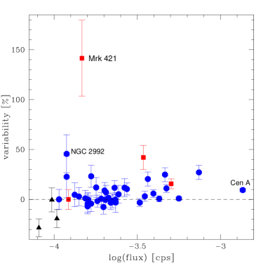
Figure 1: Variability estimator $S_{Vc}$ as a function of Swift/BAT 14–195 keV count rate. A count rate of $10^{-4}\rm\,s^{-1}$ corresponds to a flux of about $f_{14-195\rm\,keV}\simeq 6\times 10^{-11}{\rm erg}\,{\rm cm}^{-2}\,{\rm s}^{-1}$. Blazars have been marked with squares and the three objects with the lowest count rates ($<1.05\times 10^{-4}\rm\,s^{-1}$) are marked with triangles.

From Table 2 it is already apparent that none of the 11 type 1 galaxies shows significant variability, whereas of the 20 type 2 objects 50% show variability with $S_{Vc}\geq 10\%$. This effect is also apparent when comparing the variability $S_{Vc}$ with the intrinsic absorption $N_{H}$ as measured in soft X-rays (e.g. by Swift/XRT or XMM-Newton). The correlation is shown in Figure 2. Blazars have been excluded. Except for NGC 2992, none of the objects with intrinsic absorption $N_{H}<10^{22}\rm\,cm^{-2}$ shows significant variability according to the maximum likelihood estimator. NGC 2992 is also a special case because it is a Seyfert 2 galaxy with comparably low intrinsic absorption and the $N_{H}$ varies between $0.1$ and $1.0\times 10^{22}\rm\,cm^{-2}$ (Beckmann et al. 2007). Even when including NGC 2992 a Spearman rank test of $N_{H}$ versus variability gives a correlation coefficient of $r_{s}=0.31$, which corresponds to a moderate probability of correlation of $95\%$.

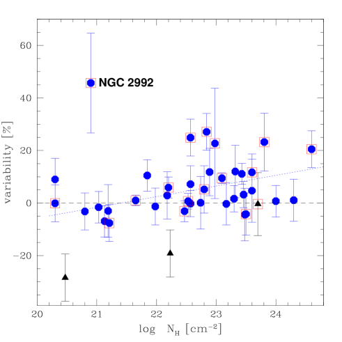
Figure 2: Variability estimator $S_{Vc}$ as a function of intrinsic absorption $N_{H}$. Blazars have been excluded and the three objects with the lowest count rates ($<1.05\times 10^{-4}\rm\,s^{-1}$) are marked with triangles. Objects enclosed by a square show a rising part of the structure function with a correlation probability of $rr_{SF}\leq 0.01$ (see Section 2.3 for details). The object with the highest $S_{Vc}$ is NGC 2992. The dotted line indicates the linear regression to the data points, excluding NGC 2992 and the three low-flux objects.

2.3 Structure Function

As an independent test for variability, we determined the structure function of the objects. Structure functions are similar to auto- and cross-correlation functions and have been introduced for analysis of radio lightcurves by Simonetti et al. (1985). Applications to other data sets have been shown, e.g. by Hughes et al. (1992), Paltani (1999), de Vries (2005), and Favre et al. (2005). The structure function is a useful and simple to use tool in order to find characteristic time scales for the variations in a source. We use the first-order structure function, which is defined as $D^{1}(\tau)=<[S(t)-S(t+\tau)]^{2}>$. Here $S(t)$ is the flux at time $t$, and $\tau$ is the time-lag, or variability time-scale. The function $D^{1}(\tau)$ can be characterized in terms of its slope: $b=d\log D^{1}/d\log\tau$. For a stationary random process the structure function is related simply to the variance $\sigma^{2}$ of the process and its autocorrelation function $\rho(\tau)$ by $D^{1}(\tau)=2\sigma^{2}[1-\rho(\tau)]$. For lags longer than the longest correlation time scale, there is an upper plateau with an amplitude equal to twice the variance of the fluctuation ($2\cdot(\sigma_{Q}^{2}+\overline{\sigma_{i}}^{2})$). For very short time lags, the structure function reaches a lower plateau which is at a level corresponding to the measurement noise ($2\cdot\overline{\sigma_{i}}^{2}$). As explained in Hughes et al. (1992), the structure function, autocorrelation function, and power spectrum density function (PSD) $P(\nu)$ are related measures of the distribution of power with time scale. If the PSD follows a power law of the form $P(\nu)\propto\nu^{-a}$, then $D^{1}(\tau)\propto\tau^{a-1}$ (Bregman et al. (1990)). For example, if $P(\nu)\propto\nu^{-1}$, then $D^{1}(\tau)\propto\tau^{0}$ (flicker noise). Flicker noise exhibits both short and long time-scale fluctuations. If $P(\nu)\propto\nu^{-2}$, then $D^{1}(\tau)\propto\tau^{1}$ (short or random walk noise). This relation is however valid only in the limit $\tau_{max}\rightarrow\infty$, $\tau_{min}\rightarrow 0$. If, on the contrary, the PSD is limited to the range $[\tau_{min},\tau_{max}]$, the relationship does not hold anymore (Paltani (1999)). This is in fact the case here, as we can probe only time scales in the range of $\tau_{min}\sim 10\rm\,days$ to $\tau_{max}\sim 100\rm\,days$. In the ideal case we can learn from the structure function of the Swift/BAT AGN about several physical properties: whether the objects show variations, what the maximum time scale of variations is, and what the type of noise is which is causing the variations. We can determine the maximum time scale $\tau_{max}$ of variability only if a plateau is reached and, in our case, if $\tau_{max}<9$ months.

Error values on the structure function have been again determined by Monte-Carlo simulation. The flux and error distribution of each source has been used. Under the assumption that the source fluxes and errors are following a Gaussian distribution, for each source 1000 lightcurves with 1 day binning have been simulated. These lightcurves have than been used to extract the structure function. The scatter in each point $D^{1}(\tau)$ is then considered when fitting a straight line to the data applying linear regression.

To test the quality of the BAT data lightcurves for determining the structure function we show in Figure 3 the one obtained for the Crab as an example for a constant source. As expected, after the structure function gets out of the noisy part at time scales shorter than $\sim 4$ days, it stays more or less constant. Thus, no variability is detected in the Crab up to time scales of the duration of the survey.

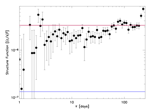
Figure 3: Structure function for Swift/BAT data of the Crab (one day binning). The upper line indicates an amplitude equal to twice the variance of the fluctuation, the lower line corresponds to the level of the average measurement noise ($2\cdot\overline{\sigma_{i}}^{2}$).

Figure 4 shows the structure function for the BAT data of NGC 4151. This source has a lower flux than the Crab, thus the noisy part of the structure function extends up to $\tau\simeq 20-40$ days. At longer time scales, the function is rising. It is not clear though whether it levels out after 150 days, which would mean there is no variability on time scales longer than 150 days. But the source is variable on timescales ranging from 3 weeks to (at least) 5 months. For comparison we checked the CGRO/BATSE Earth-occultation archive which contains light curves for 4 sources of our sample, i.e. 3C 273, Cen A, NGC 4151, and NGC 1275. Figure 5 shows the $20-70\rm\,keV$ structure function of NGC 4151 based on CGRO/BATSE data. The sampling here is worse at the time scales probed by the Swift/BAT survey, but reaches out to time scales up to $\tau\simeq 8$ years. One can see that the turnover does not appear within the probed time scale, consistent with the results we derived from the BAT data. Also for the other 3 objects the results from BATSE and BAT are consistent, showing variability for Cen A and 3C 273 over all the sampled time scales, and no variability for NGC 1275. We also checked the lightcurves for random positions in the sky. One example is shown in Figure 6.

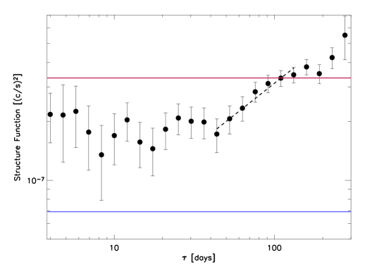
Figure 4: Structure function for Swift/BAT data of the Seyfert 1.5 galaxy NGC 4151 (one day binning). The upper and lower lines indicate $2(\sigma_{Q}^{2}+\overline{\sigma_{i}}^{2})$ and $2\overline{\sigma_{i}}^{2}$, respectively. The dashed line indicates the linear regression applied to the data, resulting in $D^{1}(\tau)\propto\tau^{0.65}$.

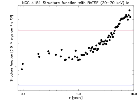
Figure 5: Structure function for CGRO/BATSE data (20 - 70 keV) of NGC 4151. The upper and lower lines indicate $2(\sigma_{Q}^{2}+\overline{\sigma_{i}}^{2})$ and $2\overline{\sigma_{i}}^{2}$, respectively.

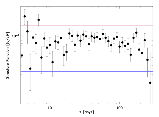
Figure 6: Structure function for Swift/BAT data of a random position in the sky (XXX J0044.1+5019). The upper and lower lines indicate $2(\sigma_{Q}^{2}+\overline{\sigma_{i}}^{2})$ and $2\overline{\sigma_{i}}^{2}$, respectively.

Based on the comparison of the structure function curves of the BAT AGN with those of the Crab and the random positions, we examined the curves of all objects of the sample presented here for rising evolution in the range $\tau=20-200\rm\,days$. Individual time limits $l_{min}$ and $l_{max}$ have been applied in order to apply a linear regression fit to the curves, taking into account the errors determined in the Monte-Carlo simulation. Therefore this method inherits a subjective element which obviously limits the usefulness of the output. On the other hand, a fixed $l_{min}$ and $l_{max}$ does not take into account the difference in significance between the sources. The $l_{max}$ applied is not necessarily the maximum time-scale of variability $\tau_{max}$, especially when $\tau_{max}>100\rm\,days$. The last column of Table 2 reports the results. $rr_{SF}$ gives the probability for a non-correlation of $\tau$ and $D^{1}(\tau)$. We consider here objects with $\log rr_{SF}\leq-2$ as variable, i.e. objects where we find a probability of $>99\%$ for correlation. The structure function of the Crab lightcurve for example results in $\log rr_{SF}=-0.6$. One can see an overall agreement with the variability estimator, although in some cases there are discrepancies, e.g. for NGC 3516 and NGC 5728, which have a rising structure function, but do not give an indication of variability in the maximum likelihood approach. In total, 16 objects show a rising structure function, and 15 objects show a variability $S_{Vc}>10\%$ in the maximum likelihood approach. 10 objects show a rising structure function and $S_{Vc}>10\%$. A Spearman rank test of the variability estimator versus the $\log rr_{SF}$ value gives a probability of $>98\%$ for correlation, and $>99.5\%$ if we ignore the objects with a negative variability estimator. Some caution has to be applied when comparing those two values: while the variability estimator measures the strength of the variability, the $\log rr_{SF}$ indicates the probability that there is indeed significant variation. A bright source can have a small but very significant variability. The fact that the variability estimator is based on 20-day binned lightcurves, while the structure functions are extracted from 1-day binned data should not affect the results strongly: because of the moderate sampling of the light curves, the structure function analysis cannot probe variability below $\sim 20\rm\,days$ in most cases.

Concerning a dependence of variability on intrinsic absorption, the structure function method confirms the tendency seen in variability estimator. As shown in Fig.2, $25\%$ of the objects with $N_{H}<10^{22}\rm\,cm^{-2}$ and $46\%$ of the objects with $N_{H}>10^{22}\rm\,cm^{-2}$ show a rising structure function. Again, this should be taken as a tendency, not as a strong correlation.

3 Discussion

Studying the correlation between absorption and variability, there is a tendency that the stronger absorbed sources are the more variable ones (Fig. 2). If the central engine in type 1 and type 2 objects is indeed similar, this is a surprising result. First, absorption should not play a major role in the spectrum at energies $>15\rm\,keV$ unless the absorption is $N_{H}\gg 10^{23}\rm\,cm^{-2}$. But most of the sources studied here show only moderate absorption with hydrogen column densities of the order of $N_{H}=10^{21}-10^{23}\rm\,cm^{-2}$. Even if absorption plays a role, the expected effect would be reverse to the observation, i.e. one would expect a damping effect of the absorption and the absorbed sources should be less variable than the unabsorbed ones. In a recent study of XMM-Newton data of AGN in the Lockman Hole by Mateos et al. (2007) it has been shown that although the fraction of variable sources is higher among type-1 than in type-2 AGN, the fraction of AGN with detected spectral variability were found to be $\sim 14\pm 8\%$ for type-1 AGN and $34\pm 14\%$ for type-2 AGN. This might indicate that the differences between type 1 and type 2 galaxies are indeed more complex than just different viewing angles resulting in a difference in the absorbing material along the line of sight. In this context, alternative and modified accretion models might be considered, such as matter accretion via clumps of matter and interaction between these clumps (Courvoisier & Türler (2005)) or star collisions in a cluster of stars orbiting around the central massive black hole (Torricelli-Ciamponi et al. (2000)).

Another explanation for the lack of variable type 1 objects in our sample could be that the correlation between absorption and variability is an indirect one, caused by two other correlations: an anti-correlation of intrinsic absorption and luminosity, and the anti-correlation of variability and luminosity. While the first dependence in the data set presented here is very weak, there is indeed a trend of lower variability for sources with higher luminosity (Fig. 7). A Spearman rank test of luminosity versus variability estimator results in a correlation coefficient of $r_{s}=-0.47$, which corresponds to a correlation probability of $>99\%$.

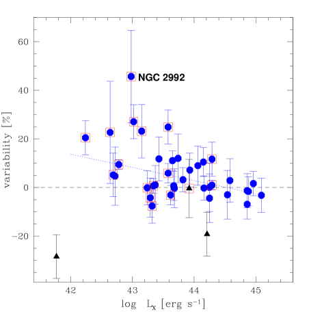
Figure 7: Variability estimator $S_{Vc}$ as a function of X-ray luminosity in the 14–195 keV band. The three objects with the lowest count rates ($<1.05\times 10^{-4}\rm\,s^{-1}$) are marked with triangles. The blazars are located outside the area covered in this plot. The dotted line indicates the linear regression to the data points.

All the sources which show a $S_{Vc}>20\%$ have luminosities of $L_{(14-195\rm\,keV)}<4\times 10^{43}\rm\,erg\,s^{-1}$, and all sources with $S_{Vc}>10\%$ have $L_{(14-195\rm\,keV)}<2\times 10^{44}\rm\,erg\,s^{-1}$. Using the results from the structure function a similar trend is seen: 76% of the objects with $L_{(14-195\rm\,keV)}<4\times 10^{43}\rm\,erg\,s^{-1}$ have a significant rising part of the structure function, whereas only 13% of the more luminous objects show this indication for variability.

The results based on the structure function have to be interpreted with caution due to the relatively small number of significant data points. Nevertheless it appears that the maximum time length $\tau_{max}$ for variability is significantly longer than in the optical and UV region. Collier & Peterson (2001) studied 4 of the objects presented here and found a $\tau_{max}$ significantly smaller in all cases for the optical and UV. The same applies for the AGN variability study performed by Favre et al. (2005) using UV data, including 7 of the objects studied here. On the contrary, de Vries et al. (2005) do not find a turn-over in optical lightcurves up to $\tau_{max}\sim 40\rm\,yr$.

The average gradient $\beta$ of the rising part of the structure functions (assuming $D^{1}(\tau)\propto\tau^{\beta}$) with $rr_{SF}<0.01$ is $\overline{\beta}=0.4\pm 0.1$ and ranging for the individual sources from $\beta=0.2$ (3C 454.3, NGC 5506, and 3C 273) to $\beta=1.0$ (ESO 506-027), consistent with measurements of the power spectrum of 11 AGN in the X-rays by EXOSAT, which resulted in $\overline{\beta}=0.55\pm 0.09$ (Lawrence & Papadakis (1993)). The average value is closer to the slope expected from disk instability models ($\beta=0.8-1.0$, Mineshige et al. (1994)), rather than to the slope of the starburst model ($\beta=1.4-1.8$, Aretxaga et al. (1997)). This result should not be overemphasized as de Vries et al. (2004) pointed out that the measurement noise does have a direct effect on the slope of the structure function. The larger the noise, the shallower the slope.

Compared to softer X-rays, the Seyfert galaxies appear to exhibit less variability than e.g. at 2–10 keV. This indicates that there is an overall tendency for an anticorrelation of variability with energy. This has been reported for some of the objects studied here e.g. for 3C 390.3 and 3C 120 (Gliozzi et al. (2002)) which show no significant variation here, and also for NGC 3227 (Uttley & McHardy 2005). In the latter article the case of NGC 5506 is also described in which this trend is reversed in the soft X-rays. This object does not show significant variability applying the maximum likelihood estimator, but shows indeed a rising structure function with $\tau_{max}\mathrel{>\kern-10.00002pt\lower 3.87495pt\hbox{$\sim$}}200$ days.

The fraction of variable objects in our study is about $30\%$ among the Seyfert type AGN according to both methods, the variability estimator and the structure function. This is a lower fraction than detected at softer X-rays. For example among the AGN in the Chandra Deep Field South 60% of the objects show variability (Bauer et al. (2004)), and XMM-Newton data of the Lockman Hole reveal a 50% fraction (Mateos et al. (2007)). Part of the lower variability detected in the Swift/BAT AGN sample might be due to the lower statistics apparent in the lightcurves when compared to the soft X-ray data. Bauer et al. (2004) pointed out that the fraction of variable sources is indeed a function of source brightness and rises up to $80-90\%$ for better photon statistics and also Mateos et al. find $>80\%$ of the AGN variable for the best quality light curves. Within our sample we are not able to confirm this trend, which might be due to the small size of the sample.

An anticorrelation of X-ray variability with luminosity in AGN has been reported before for energies $<10\rm\,keV$ (e.g. Barr & Mushotzky 1986, Lawrence & Papadakis 1993) and has been also seen in the UV range (Paltani & Courvoisier (1994)) and in the optical domain (de Vries et al. (2005)), although narrow-line Seyfert 1 galaxies apparently show the opposite behaviour (e.g. Turner et al. 1999). As only one of the objects (NGC 4051) discussed here is a NLSy1 galaxy, we detect a continuous effect from soft to hard X-rays, which indeed indicates that the dominant underlying physical process at $\sim 5\rm\,keV$ is the same as at $\sim 20\rm\,keV$. In a more recent study, Papadakis (2004) reported that this correlation is in fact based on the connection between luminosity and the mass of the central black hole $M_{BH}$. This may be explained if more luminous sources are physically larger in size, so that they are actually varying more slowly. Alternatively, they may contain more independently flaring regions and so have a genuinely lower amplitude. The observed correlation might reflect the anticorrelation of variability and black hole mass. In the case of the sample presented here, such an anticorrelation is not detectable, but it has to be pointed out that estimates for $M_{BH}$ are only available for 13 objects. In addition, the range of objects in luminosity and black hole mass might be too small in order to detect such a trend. Uttley & McHardy (2004) explained the anti-correlation of variability and $M_{BH}$ by assuming that the X-rays are presumably produced in optically thin material close to the central black hole, at similar radii (i.e. in Schwarzschild radii, $R_{S}$) in different AGN. As $R_{S}=2GM_{BH}c^{-2}$, longer time scales for the variability are expected for the more massive central engines, making the objects less variable on a monthly time scale studied here.

4 Conclusions

We presented the variability analysis of the brightest AGN seen by Swift/BAT, using two ways of analysis: a maximum-likelihood variability estimator and the structure function. Both methods show that $\sim 30\%$ of the Seyfert type AGN exhibit significant variability on the time scale of $20-150\rm\,days$. The analysis indicates that the type 1 galaxies are less variable than the type 2 type ones, and that unabsorbed sources are less variable than absorbed ones. With higher significance we detect an anti-correlation of luminosity and variability. No object with luminosity $L_{X}>5\times 10^{43}\rm\,erg\,s^{-1}$ shows strong variability. The anti-correlation might either be caused by intrinsic differences between the central engine in Seyfert 1 and Seyfert 2 galaxies, or it might be connected to the same anti-correlation seen already at softer X-rays, in the UV and in the optical band. Further investigations on this subject are necessary in order to clarify whether one can treat the AGN as an upscale version of Galactic black hole systems (e.g. Vaughan, Fabian & Iwasawa 2005).

The data presented here do not allow a final conclusion on this point. The correlations are still too weak and for too many objects it is not possible to determine the strength of the intrinsic variability. Similar studies at softer X-rays seem to indicate that with increasing statistics we will be able to detect significant variability in a larger fraction of objects. The study presented here will be repeated as soon as significantly more Swift/BAT data are available for analysis. As this study was based on 9 months of data, a ten times larger data set will be available in 2012. Eventually, the data will allow more sophisticated analysis, such as the construction of power density spectra. In addition the same analysis can be applied to INTEGRAL (Winkler et al. (2003)) IBIS/ISGRI data. Although INTEGRAL does not achieve a sky coverage as homogeneous as Swift/BAT, it allows a more detailed analysis of some AGN in specific regions, e.g. along the Galactic plane.

The combination of results from both missions, Swift and INTEGRAL, should allow us to verify whether indeed Seyfert 2 galaxies are more variable at hard X-rays than the unabsorbed Seyfert 1, and whether this points to intrinsic differences in the two AGN types.