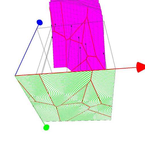
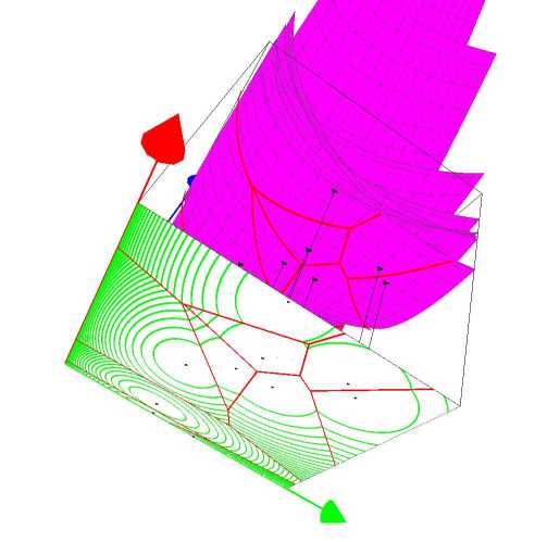
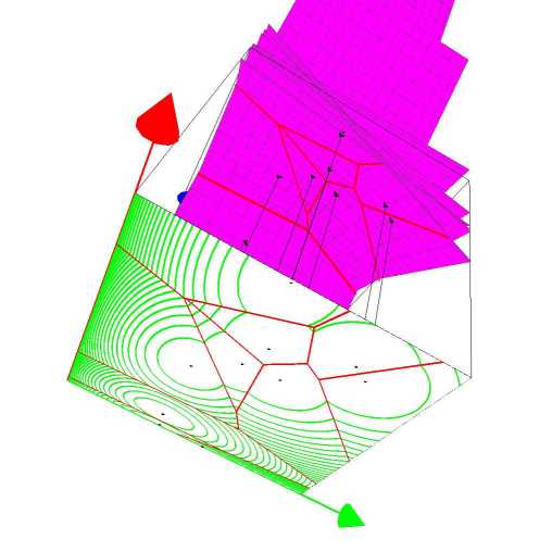
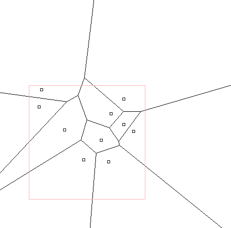
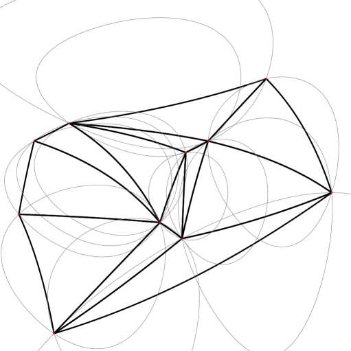
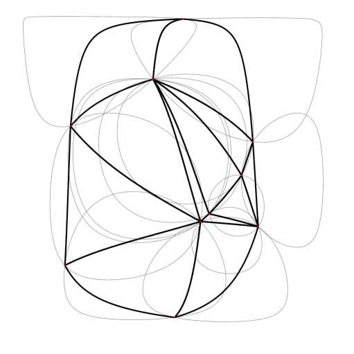
Bregman Voronoi Diagrams: Properties, Algorithms and Applicationsthanks: A preliminary version appeared in the 18th ACM-SIAM Symposium on Discrete Algorithms (SODA), pp. 746-755, 2007. Related materials are available online at http://www.csl.sony.co.jp/person/nielsen/BregmanVoronoi/ — Version for arXiv (small resolution jpg/png files).

Frank Nielsen Sony Computer Science Laboratories Inc., Fundamental Research Laboratory, Japan.    Jean-Daniel Boissonnat INRIA Sophia-Antipolis, GEOMETRICA, France.    Richard Nock Université Antilles-Guyane, CEREGMIA, France.
Abstract

The Voronoi diagram of a finite set of objects is a fundamental geometric structure that subdivides the embedding space into regions, each region consisting of the points that are closer to a given object than to the others. We may define many variants of Voronoi diagrams depending on the class of objects, the distance functions and the embedding space. In this paper, we investigate a framework for defining and building Voronoi diagrams for a broad class of distance functions called Bregman divergences. Bregman divergences include not only the traditional (squared) Euclidean distance but also various divergence measures based on entropic functions. Accordingly, Bregman Voronoi diagrams allow to define information-theoretic Voronoi diagrams in statistical parametric spaces based on the relative entropy of distributions. We define several types of Bregman diagrams, establish correspondences between those diagrams (using the Legendre transformation), and show how to compute them efficiently. We also introduce extensions of these diagrams, e.g. k𝑘k-order and k𝑘k-bag Bregman Voronoi diagrams, and introduce Bregman triangulations of a set of points and their connexion with Bregman Voronoi diagrams. We show that these triangulations capture many of the properties of the celebrated Delaunay triangulation. Finally, we give some applications of Bregman Voronoi diagrams which are of interest in the context of computational geometry and machine learning.

Categories and Subject Descriptors: I.3.5 [Computer Graphics] Computational Geometry and Object Modeling — Geometric algorithms, languages, and systems; F.2.2 [Analysis of Algorithms and Problem Complexity]: Nonnumerical Algorithms and Problems — Geometrical problems and computations; G.2.1 [Discrete Mathematics]: Combinatorics.

General Terms: Algorithms, Theory

Keywords: Computational Information Geometry, Voronoi diagram, Delaunay triangulation, Bregman divergence, Bregman ball, Legendre transformation, Quantification, Sampling, Clustering

1 Introduction and prior work

The Voronoi diagram vor(𝒮)vor𝒮\mathrm{vor}(\mathcal{S}) of a set of n𝑛n points 𝒮={𝐩1,,𝐩n}𝒮subscript𝐩1subscript𝐩𝑛\mathcal{S}=\{\mathbf{p}_{1},...,\mathbf{p}_{n}\} of the d𝑑d-dimensional Euclidean space dsuperscript𝑑\mathbb{R}^{d} is defined as the cell complex whose d𝑑d-cells are the Voronoi regions {vor(𝐩i)}i{1,..,n}\{\mathrm{vor}(\mathbf{p}_{i})\}_{i\in\{1,..,n\}} where vor(𝐩i)vorsubscript𝐩𝑖\mathrm{vor}(\mathbf{p}_{i}) is the set of points of dsuperscript𝑑\mathbb{R}^{d} closer to 𝐩isubscript𝐩𝑖\mathbf{p}_{i} than to any other point of 𝒮𝒮\mathcal{S} with respect to a distance function δ𝛿\delta:

vor(𝐩i)=def{𝐱d|δ(𝐩i,𝐱)δ(𝐩j,𝐱)𝐩j𝒮}.superscriptdefvorsubscript𝐩𝑖conditional-set𝐱superscript𝑑𝛿subscript𝐩𝑖𝐱𝛿subscript𝐩𝑗𝐱for-allsubscript𝐩𝑗𝒮\mathrm{vor}(\mathbf{p}_{i})\stackrel{{\scriptstyle\mathrm{def}}}{{=}}\{\mathbf{x}\in\mathbb{R}^{d}\ |\ \delta(\mathbf{p}_{i},\mathbf{x})\leq\delta(\mathbf{p}_{j},\mathbf{x})\ \forall\ \mathbf{p}_{j}\in\mathcal{S}\}.

Points {𝐩i}isubscriptsubscript𝐩𝑖𝑖\{\mathbf{p}_{i}\}_{i} are called the Voronoi sites or Voronoi generators. Since its inception in disguise by Descartes in the 17th century [5], Voronoi diagrams have found a broad spectrum of applications in science. Computational geometers have focused at first on Euclidean Voronoi diagrams [5] by considering the case where δ(𝐱,𝐲)𝛿𝐱𝐲\delta(\mathbf{x},\mathbf{y}) is the Euclidean distance 𝐱𝐲=i=1d(xiyi)2norm𝐱𝐲superscriptsubscript𝑖1𝑑superscriptsubscript𝑥𝑖subscript𝑦𝑖2||\mathbf{x}-\mathbf{y}||=\sqrt{\sum_{i=1}^{d}(x_{i}-y_{i})^{2}}. Voronoi diagrams have been later on defined and studied for other distance functions, most notably the L1subscript𝐿1L_{1} distance 𝐱𝐲1=i=1d|xiyi|subscriptnorm𝐱𝐲1superscriptsubscript𝑖1𝑑subscript𝑥𝑖subscript𝑦𝑖||\mathbf{x}-\mathbf{y}||_{1}=\sum_{i=1}^{d}|x_{i}-y_{i}| (Manhattan distance) and the Lsubscript𝐿L_{\infty} distance 𝐱𝐲=maxi{1,,d}|xiyi|subscriptnorm𝐱𝐲subscript𝑖1𝑑subscript𝑥𝑖subscript𝑦𝑖||\mathbf{x}-\mathbf{y}||_{\infty}=\max_{i\in\{1,...,d\}}|x_{i}-y_{i}| [10, 5]. Klein further presented an abstract framework for describing and computing the fundamental structures of abstract Voronoi diagrams [26, 11].
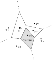
Refer to caption
Figure 1: Ordinary Euclidean Voronoi diagram of a given set 𝒮𝒮\mathcal{S} of seven sites. In the bounded Voronoi cell vor(𝐩6)vorsubscript𝐩6\mathrm{vor}(\mathbf{p}_{6}), every point 𝐩vor(𝐩6)𝐩vorsubscript𝐩6\mathbf{p}\in\mathrm{vor}(\mathbf{p}_{6}) is closer to 𝐩6subscript𝐩6\mathbf{p}_{6} than to any other site of 𝒮𝒮\mathcal{S} (with respect to the Euclidean distance). Dashed segments denote infinite edges delimiting unbounded cells.

In artificial intelligence, machine learning techniques also rely on geometric concepts for building classifiers in supervised problems (e.g., linear separators, oblique decision trees, etc.) or clustering data in unsupervised settings (e.g., k𝑘k-means, support vector clustering [2], etc.). However, the considered data sets 𝒮𝒮\mathcal{S} and their underlying spaces 𝒳𝒳\mathcal{X} are usually not metric spaces. The notion of distance between two elements of 𝒳𝒳\mathcal{X} needs to be replaced by a pseudo-distance that is not necessarily symmetric and may not satisfy the triangle inequality. Such a pseudo-distance is also referred to as distortion, (dis)similarity or divergence in the literature. For example, in parametric statistical spaces 𝒳𝒳\mathcal{X}, a vector point represent a distribution and its coordinates store the parameters of the associated distribution. A notion of “distance” between two such points is then needed to represent the divergence between the corresponding distributions.

Very few works have tackled an in-depth study of Voronoi diagrams and their applications for such a kind of statistical spaces. This is all the more important even for ordinary Voronoi diagrams as Euclidean point location of sites are usually observed in noisy environments (e.g., imprecise point measures in computer vision experiments), and “noise” is often modeled by means of Normal distributions (so-called “Gaussian noise”). To the best of our knowledge, statistical Voronoi diagrams have only been considered in a 4-page short paper of Onishi and Imai [34] which relies on Kullback-Leibler divergence of d𝑑dD multivariate normal distributions to study combinatorics of their Voronoi diagrams, and subsequently in a 2-page video paper of Sadakane et al. [40] which defines the divergence implied by a convex function and its conjugate, and present the Voronoi diagram with flavors of information geometry [1] (see also [35] and related short communications [25, 24]). Our study of Bregman Voronoi diagrams generalizes and subsumes these preliminary studies using an easier concept of divergence: Bregman divergences [12, 6] that do not rely explicitly on convex conjugates. Bregman divergences encapsulate the squared Euclidean distance and many widely used divergences, e.g. the Kullback-Leibler divergence. It should be noticed however that other divergences have been defined and studied in the context of Riemannian geometry [1]. Sacrifying for some generality, while not very restrictive in practice, allows a much simpler treatment and our study of Bregman divergences is elementary and does not rely on Riemannian geometry.

In this paper, we give a thorough treatment of Bregman Voronoi diagrams which elegantly unifies the ordinary Euclidean Voronoi diagram and statistical Voronoi diagrams. Our contributions are summarized as follows:

  • Since Bregman divergences are not symmetric, we define two types of Bregman Voronoi diagrams. One is an affine diagram with convex polyhedral cells while the other one is curved. The cells of those two diagrams are in 1-1 correspondence through the Legendre transformation. We also introduce a third-type symmetrized Bregman Voronoi diagram.

  • We present a simple way to compute the Bregman Voronoi diagram of a set of points by lifting the points in a higher dimensional space using an extra dimension. This mapping leads also to combinatorial bounds on the size of these diagrams. We also define weighted Bregman Voronoi diagrams and show that the class of these diagrams is identical to the class of affine (or power) diagrams. Special cases of weighted Bregman Voronoi diagrams are the k𝑘k-order and k𝑘k-bag Bregman Voronoi diagrams.

  • We define two triangulations of a set of points. The first one captures some of the most important properties of the well-known Delaunay triangulation. The second triangulation is called a geodesic Bregman triangulation since its edges are geodesic arcs. Differently from the first triangulation, this triangulation is the geometric dual of the first-type Bregman Voronoi diagram of its vertices.

  • We give a few applications of Bregman Voronoi diagrams which are of interest in the context of computational geometry and machine learning.

The outline of the paper is as follows: In Section 2, we define Bregman divergences and recall some of their basic properties. In Section 3, we study the geometry of Bregman spaces and characterize bisectors, balls and geodesics. Section 4 is devoted to Bregman Voronoi diagrams and Section 5 to Bregman triangulations. In Section 6, we select of few applications of interest in computational geometry and machine learning. Finally, Section 7 concludes the paper and mention further ongoing investigations.

Notations.

In the whole paper, 𝒳𝒳\mathcal{X} denotes an open convex domain of dsuperscript𝑑\mathbb{R}^{d} and F:𝒳:𝐹maps-to𝒳F:\mathcal{X}\mapsto\mathbb{R} a strictly convex and differentiable function. \mathcal{F} denotes the graph of F𝐹F, i.e. the set of points (𝐱,z)𝒳×𝐱𝑧𝒳(\mathbf{x},z)\in\mathcal{X}\times\mathbb{R} where z=F(𝐱)𝑧𝐹𝐱z=F(\mathbf{x}). We write 𝐱^^𝐱\hat{\mathbf{x}} for the point (𝐱,F(𝐱))𝐱𝐹𝐱(\mathbf{x},F(\mathbf{x}))\in\mathcal{F}. Fbold-∇𝐹{{\bm{\nabla}}F}, 2Fsuperscriptbold-∇2𝐹{{\bm{\nabla}^{2}F}} and 1Fsuperscriptbold-∇1𝐹{{\bm{\nabla}^{-1}F}} denote respectively the gradient, the Hessian and the inverse gradient of F𝐹F.

2 Bregman divergences

In this section, we recall the definition of Bregman111Lev M. Bregman historically pioneered this notion in the seminal work [12] on minimization of a convex objective function under linear constraints. See http://www.math.bgu.ac.il/serv/segel/bregman.html. We gratefully acknowledge him for sending us this historical paper. divergences and some of their main properties (§2.1). We show that the notion of Bregman divergence encapsulates the squared Euclidean distance as well as several well-known information-theoretic divergences. We introduce the notion of dual divergences (§2.2) and show how this comes in handy for symmetrizing Bregman divergences (§2.3). Finally, we prove that the Kullback-Leibler divergence of distributions that belong to the exponential family of distributions can be viewed as a Bregman divergence (§2.4).

2.1 Definition and basic properties

For any two points 𝐩𝐩\mathbf{p} and 𝐪𝐪\mathbf{q} of 𝒳d𝒳superscript𝑑\mathcal{X}\subseteq\mathbb{R}^{d}, the Bregman divergence222See Java™ applet at http://www.csl.sony.co.jp/person/nielsen/BregmanDivergence/ DF(||):𝒳D_{F}(\cdot||\cdot):\mathcal{X}\mapsto\mathbb{R} of 𝐩𝐩\mathbf{p} to 𝐪𝐪\mathbf{q} associated to a strictly convex and differentiable function F𝐹F (called the generator function of the divergence) is defined as

DF(𝐩||𝐪)=defF(𝐩)F(𝐪)F(𝐪),𝐩𝐪,D_{F}(\mathbf{p}||\mathbf{q})\stackrel{{\scriptstyle\mathrm{def}}}{{=}}F(\mathbf{p})-F(\mathbf{q})-{\langle{{{\bm{\nabla}}F}(\mathbf{q})},{\mathbf{p}-\mathbf{q}}\rangle}, (1)

where F=[Fx1Fxd]Tbold-∇𝐹superscriptdelimited-[]𝐹subscript𝑥1𝐹subscript𝑥𝑑𝑇{{\bm{\nabla}}F}=[\frac{\partial F}{\partial x_{1}}\ ...\ \frac{\partial F}{\partial x_{d}}]^{T} denotes the gradient operator, and 𝐩,𝐪𝐩𝐪{\langle{\mathbf{p}},{\mathbf{q}}\rangle} the inner (or dot) product: i=1dpiqisuperscriptsubscript𝑖1𝑑subscript𝑝𝑖subscript𝑞𝑖\sum_{i=1}^{d}p_{i}q_{i}.

Informally speaking, Bregman divergence DFsubscript𝐷𝐹D_{F} is the tail of the Taylor expansion of F𝐹F. See [16] for an axiomatic characterization of Bregman divergences as “permissible” divergences.

Lemma 1

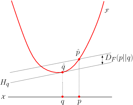
The Bregman divergence DF(𝐩||𝐪)D_{F}(\mathbf{p}||\mathbf{q}) is geometrically measured as the vertical distance between 𝐩^^𝐩\hat{\mathbf{p}} and the hyperplane H𝐪subscript𝐻𝐪H_{\mathbf{q}} tangent to \mathcal{F} at point 𝐪^^𝐪\hat{\mathbf{q}}: DF(𝐩||𝐪)=F(𝐩)H𝐪(𝐩)D_{F}(\mathbf{p}||\mathbf{q})=F(\mathbf{p})-H_{\mathbf{q}}(\mathbf{p}).

Proof: The tangent hyperplane to hypersurface :z=F(𝐱):𝑧𝐹𝐱\mathcal{F}:z=F(\mathbf{x}) at point 𝐪^^𝐪\hat{\mathbf{q}} is H𝐪:z=F(𝐪)+F(𝐪),𝐱𝐪:subscript𝐻𝐪𝑧𝐹𝐪bold-∇𝐹𝐪𝐱𝐪H_{\mathbf{q}}:z=F(\mathbf{q})+{\langle{{{\bm{\nabla}}F}(\mathbf{q})},{\mathbf{x}-\mathbf{q}}\rangle}. It follows that DF(𝐩||𝐪)=F(𝐩)H𝐪(𝐩)D_{F}(\mathbf{p}||\mathbf{q})=F(\mathbf{p})-H_{\mathbf{q}}(\mathbf{p}) (see Figure 2). \square

Refer to caption
Figure 2: Visualizing the Bregman divergence. DF(.||𝐪)D_{F}(.||\mathbf{q}) is the vertical distance between \mathcal{F} and the hyperplane tangent to \mathcal{F} at 𝐪^^𝐪\hat{\mathbf{q}}.

We now give some basic properties of Bregman divergences. The first property seems to be new. The others are well known. First, observe that, for most functions F𝐹F, the associated Bregman divergence is not symmetric, i.e. DF(𝐩||𝐪)DF(𝐪||𝐩)D_{F}(\mathbf{p}||\mathbf{q})\not=D_{F}(\mathbf{q}||\mathbf{p}) (the symbol |||| is put to emphasize this point, as is standard in information theory). The following lemma proves this claim.

Lemma 2

Let F𝐹F be properly defined for DFsubscript𝐷𝐹D_{F} to exist. Then DFsubscript𝐷𝐹D_{F} is symmetric if and only if the Hessian 2Fsuperscriptbold-∇2𝐹{{\bm{\nabla}^{2}F}} is constant on 𝒳𝒳{\mathcal{X}}.

Proof: (\Rightarrow) From Eq. 1, the symmetry DF(𝐩||𝐪)=DF(𝐪||𝐩)D_{F}(\mathbf{p}||\mathbf{q})=D_{F}(\mathbf{q}||\mathbf{p}) yields:

F(𝐩)𝐹𝐩\displaystyle F(\mathbf{p}) =\displaystyle= F(𝐪)+12𝐩𝐪,F(𝐪)+F(𝐩).𝐹𝐪12𝐩𝐪bold-∇𝐹𝐪bold-∇𝐹𝐩\displaystyle F(\mathbf{q})+\frac{1}{2}\langle\mathbf{p}-\mathbf{q},{{\bm{\nabla}}F}(\mathbf{q})+{{\bm{\nabla}}F}(\mathbf{p})\rangle\>\>. (2)

A Taylor expansion of F𝐹F around 𝐪𝐪\mathbf{q} using the Lagrange form of the remainder also yields:

F(𝐩)𝐹𝐩\displaystyle F(\mathbf{p}) =\displaystyle= F(𝐪)+𝐩𝐪,F(𝐪)+12(𝐩𝐪)T2F(𝐪)(𝐩𝐪)+16𝐩𝐪,F3(𝐫𝐩𝐪),𝐹𝐪𝐩𝐪bold-∇𝐹𝐪12superscript𝐩𝐪𝑇superscriptbold-∇2𝐹𝐪𝐩𝐪16superscript𝐩𝐪bold-∇𝐹3subscript𝐫𝐩𝐪\displaystyle F(\mathbf{q})+\langle\mathbf{p}-\mathbf{q},{{\bm{\nabla}}F}(\mathbf{q})\rangle+\frac{1}{2}(\mathbf{p}-\mathbf{q})^{T}{{\bm{\nabla}^{2}F}}(\mathbf{q})(\mathbf{p}-\mathbf{q})+\frac{1}{6}\langle\mathbf{p}-\mathbf{q},{{\bm{\nabla}}F}\rangle^{3}(\mathbf{r}_{\mathbf{p}\mathbf{q}})\>\>, (3)

with 𝐫𝐩𝐪subscript𝐫𝐩𝐪\mathbf{r}_{\mathbf{p}\mathbf{q}} on the line segment 𝐩𝐪𝐩𝐪\mathbf{p}\mathbf{q}. Equations (2) and (3) yield the following constraint:

𝐩𝐪,F(𝐩)𝐩𝐪bold-∇𝐹𝐩\displaystyle\langle\mathbf{p}-\mathbf{q},{{\bm{\nabla}}F}(\mathbf{p})\rangle =\displaystyle= 𝐩𝐪,F(𝐪)+(𝐩𝐪)T2F(𝐪)(𝐩𝐪)+13𝐩𝐪,F3(𝐫𝐩𝐪).𝐩𝐪bold-∇𝐹𝐪superscript𝐩𝐪𝑇superscriptbold-∇2𝐹𝐪𝐩𝐪13superscript𝐩𝐪bold-∇𝐹3subscript𝐫𝐩𝐪\displaystyle\langle\mathbf{p}-\mathbf{q},{{\bm{\nabla}}F}(\mathbf{q})\rangle+(\mathbf{p}-\mathbf{q})^{T}{{\bm{\nabla}^{2}F}}(\mathbf{q})(\mathbf{p}-\mathbf{q})+\frac{1}{3}\langle\mathbf{p}-\mathbf{q},{{\bm{\nabla}}F}\rangle^{3}(\mathbf{r}_{\mathbf{p}\mathbf{q}})\>\>. (4)

On the other hand, if we make the Taylor expansion of Fbold-∇𝐹{{\bm{\nabla}}F} around 𝐪𝐪\mathbf{q} and then multiply both sides by 𝐩𝐪𝐩𝐪\mathbf{p}-\mathbf{q}, we separately obtain:

𝐩𝐪,F(𝐩)𝐩𝐪bold-∇𝐹𝐩\displaystyle\langle\mathbf{p}-\mathbf{q},{{\bm{\nabla}}F}(\mathbf{p})\rangle =\displaystyle= 𝐩𝐪,F(𝐪)+(𝐩𝐪)T2F(𝐪)(𝐩𝐪)+12𝐩𝐪,F3(𝐬𝐩𝐪),𝐩𝐪bold-∇𝐹𝐪superscript𝐩𝐪𝑇superscriptbold-∇2𝐹𝐪𝐩𝐪12superscript𝐩𝐪bold-∇𝐹3subscript𝐬𝐩𝐪\displaystyle\langle\mathbf{p}-\mathbf{q},{{\bm{\nabla}}F}(\mathbf{q})\rangle+(\mathbf{p}-\mathbf{q})^{T}{{\bm{\nabla}^{2}F}}(\mathbf{q})(\mathbf{p}-\mathbf{q})+\frac{1}{2}\langle\mathbf{p}-\mathbf{q},{{\bm{\nabla}}F}\rangle^{3}(\mathbf{s}_{\mathbf{p}\mathbf{q}})\>\>,

with 𝐬𝐩𝐪subscript𝐬𝐩𝐪\mathbf{s}_{\mathbf{p}\mathbf{q}} on the line segment 𝐩𝐪𝐩𝐪\mathbf{p}\mathbf{q}. However, for this to equal Eq. (4), we must have 𝐩𝐪,F3(𝐫𝐩𝐪)=(3/2)𝐩𝐪,F3(𝐬𝐩𝐪)superscript𝐩𝐪bold-∇𝐹3subscript𝐫𝐩𝐪32superscript𝐩𝐪bold-∇𝐹3subscript𝐬𝐩𝐪\langle\mathbf{p}-\mathbf{q},{{\bm{\nabla}}F}\rangle^{3}(\mathbf{r}_{\mathbf{p}\mathbf{q}})=(3/2)\langle\mathbf{p}-\mathbf{q},{{\bm{\nabla}}F}\rangle^{3}(\mathbf{s}_{\mathbf{p}\mathbf{q}}) for each 𝐩𝐩\mathbf{p} and 𝐪𝐪\mathbf{q} in 𝒳𝒳{\mathcal{X}}. If we pick 𝐩𝐩\mathbf{p} and 𝐪𝐪\mathbf{q} very close to each other, this equality cannot be true, except when the third differentials are all zero on 𝐫𝐩𝐪subscript𝐫𝐩𝐪\mathbf{r}_{\mathbf{p}\mathbf{q}} and 𝐬𝐩𝐪subscript𝐬𝐩𝐪\mathbf{s}_{\mathbf{p}\mathbf{q}}. Repeating this argument over each subset of 𝒳𝒳\mathcal{X} having non zero measure, we obtain that the third differentials of F𝐹F must be zero everywhere but on subsets of 𝒳𝒳\mathcal{X} with zero measure, which implies that the second differentials (the Hessian of F𝐹F, 2Fsuperscriptbold-∇2𝐹{{\bm{\nabla}^{2}F}}) are constant everywhere on 𝒳𝒳\mathcal{X}.

(\Leftarrow) Assume the hessian 2Fsuperscriptbold-∇2𝐹{{\bm{\nabla}^{2}F}} is constant on 𝒳𝒳\mathcal{X}. In this case, because F𝐹F is strictly convex, the Hessian 2Fsuperscriptbold-∇2𝐹{{\bm{\nabla}^{2}F}} is positive definite, and we can factor it as 2F=𝐏1𝐃𝐏superscriptbold-∇2𝐹superscript𝐏1𝐃𝐏{{\bm{\nabla}^{2}F}}=\mathbf{P}^{-1}\mathbf{D}\mathbf{P} where 𝐃𝐃\mathbf{D} is a diagonal matrix and 𝐏𝐏\mathbf{P} a unitary rotation matrix. Reasoning in the basis of 𝒳𝒳{\mathcal{X}} formed by 𝐏𝐏\mathbf{P}, each element 𝐱𝐱\mathbf{x} is mapped to 𝐏𝐱𝐏𝐱\mathbf{P}\mathbf{x}, and we have F(𝐱)=idixi2𝐹𝐱subscript𝑖subscript𝑑𝑖subscriptsuperscript𝑥2𝑖F(\mathbf{x})=\sum_{i}{d_{i}x^{2}_{i}}, where the disubscript𝑑𝑖d_{i}’s are the diagonal coefficients of 𝐃𝐃\mathbf{D}. The symmetry of DFsubscript𝐷𝐹D_{F} is then immediate (i.e., DFsubscript𝐷𝐹D_{F} is a generalized quadratic distance). \square

Property 1 (Non-negativity)

The strict convexity of generator function F𝐹F implies that, for any 𝐩𝐩\mathbf{p} and 𝐪𝐪\mathbf{q} in 𝒳𝒳\mathcal{X}, DF(𝐩||𝐪)0D_{F}(\mathbf{p}||\mathbf{q})\geq 0, with DF(𝐩||𝐪)=0D_{F}(\mathbf{p}||\mathbf{q})=0 if and only if 𝐩=𝐪𝐩𝐪\mathbf{p}=\mathbf{q}.

Property 2 (Convexity)

Function DF(𝐩||𝐪)D_{F}(\mathbf{p}||\mathbf{q}) is convex in its first argument 𝐩𝐩\mathbf{p} but not necessarily in its second argument 𝐪𝐪\mathbf{q}.

Bregman divergences can easily be constructed from simpler ones. For instance, multivariate Bregman divergences DFsubscript𝐷𝐹D_{F} can be created from univariate generator functions coordinate-wise as F(𝐱)=i=1dfi(xi)𝐹𝐱superscriptsubscript𝑖1𝑑subscript𝑓𝑖subscript𝑥𝑖F(\mathbf{x})=\sum_{i=1}^{d}f_{i}(x_{i}) with F=[df1dx1dfddxd]Tbold-∇𝐹superscriptdelimited-[]dsubscript𝑓1dsubscript𝑥1dsubscript𝑓𝑑dsubscript𝑥𝑑𝑇{{\bm{\nabla}}F}=[\frac{\mathrm{d}f_{1}}{\mathrm{d}x_{1}}\ ...\ \frac{\mathrm{d}f_{d}}{\mathrm{d}x_{d}}]^{T}.

Because positive linear combinations of strictly convex and differentiable functions are strictly convex and differentiable functions, new generator functions (and corresponding Bregman divergences) can also be built as positive linear combinations of elementary generator functions. This is an important property as it allows to handle mixed data sets of heterogenous types in a unified framework.

Property 3 (Linearity)

Bregman divergence is a linear operator, i.e., for any two strictly convex and differentiable functions F1subscript𝐹1F_{1} and F2subscript𝐹2F_{2} defined on 𝒳𝒳\mathcal{X} and for any λ0𝜆0\lambda\geq 0:

DF1+λF2(𝐩||𝐪)=DF1(𝐩||𝐪)+λDF2(𝐩||𝐪).D_{F_{1}+\lambda F_{2}}(\mathbf{p}||\mathbf{q})=D_{F_{1}}(\mathbf{p}||\mathbf{q})+\lambda D_{F_{2}}(\mathbf{p}||\mathbf{q}).
Property 4 (Invariance under linear transforms)

G(𝐱)=F(𝐱)+𝐚,𝐱+b𝐺𝐱𝐹𝐱𝐚𝐱𝑏G(\mathbf{x})=F(\mathbf{x})+{\langle{\mathbf{a}},{\mathbf{x}}\rangle}+b, with 𝐚d𝐚superscript𝑑\mathbf{a}\in\mathbb{R}^{d} and b𝑏b\in\mathbb{R}, is a strictly convex and differentiable function on 𝒳𝒳\mathcal{X}, and DG(𝐩||𝐪)=DF(𝐩||𝐪)D_{G}(\mathbf{p}||\mathbf{q})=D_{F}(\mathbf{p}||\mathbf{q}).

Examples of Bregman divergences are the squared Euclidean distance (obtained for F(𝐱)=𝐱2𝐹𝐱superscriptnorm𝐱2F(\mathbf{x})=\|\mathbf{x}\|^{2} and the generalized quadratic distance function F(𝐱)=𝐱T𝐐𝐱𝐹𝐱superscript𝐱𝑇𝐐𝐱F(\mathbf{x})=\mathbf{x}^{T}\mathbf{Q}\mathbf{x} where 𝐐𝐐\mathbf{Q} is a positive definite matrix. When 𝐐𝐐\mathbf{Q} is taken to be the inverse of the variance-covariance matrix, DFsubscript𝐷𝐹D_{F} is the Mahalanobis distance, extensively used in computer vision. More importantly, the notion of Bregman divergence encapsulates various information measures based on entropic functions such as the Kullback-Leibler divergence based on the (unnormalized) Shannon entropy, or the Itakura-Saito divergence based on Burg entropy (commonly used in sound processing). Table 1 lists the main univariate Bregman divergences.

Dom. 𝒳𝒳\mathcal{X} Function F𝐹F Gradient Inv. grad. Divergence DF(p||q)D_{F}(p||q)
\mathbb{R} Squared function Squared loss (norm)
x2superscript𝑥2x^{2} 2x2𝑥2x x2𝑥2\frac{x}{2} (pq)2superscript𝑝𝑞2(p-q)^{2}
+,αsubscript𝛼{\mathbb{R}}_{+},\alpha\in\mathbb{N} Norm-like Norm-like
α>1𝛼1\alpha>1 xαsuperscript𝑥𝛼x^{\alpha} αxα1𝛼superscript𝑥𝛼1\alpha x^{\alpha-1} (xα)1α1superscript𝑥𝛼1𝛼1(\frac{x}{\alpha})^{\frac{1}{\alpha-1}} pα+(α1)qααpqα1superscript𝑝𝛼𝛼1superscript𝑞𝛼𝛼𝑝superscript𝑞𝛼1p^{\alpha}+(\alpha-1)q^{\alpha}-\alpha pq^{\alpha-1}
+superscript\mathbb{R}^{+} Unnorm. Shannon entropy Kullback-Leibler div. (I-div.)
xlogxx𝑥𝑥𝑥x\log x-x logx𝑥\log x exp(x)𝑥\exp(x) plogpqp+q𝑝𝑝𝑞𝑝𝑞p\log\frac{p}{q}-p+q
Exponential Exponential loss
\mathbb{R} expx𝑥\exp x expx𝑥\exp x logx𝑥\log x exp(p)(pq+1)exp(q)𝑝𝑝𝑞1𝑞\exp(p)-(p-q+1)\exp(q)
+\mathbb{R}^{+}* Burg entropy Itakura-Saito divergence
logx𝑥-\log x 1x1𝑥-\frac{1}{x} 1x1𝑥-\frac{1}{x} pqlogpq1𝑝𝑞𝑝𝑞1\frac{p}{q}-\log\frac{p}{q}-1
[0,1]01[0,1] Bit entropy Logistic loss
xlogx+(1x)log(1x)𝑥𝑥1𝑥1𝑥x\log x+(1-x)\log(1-x) logx1x𝑥1𝑥\log\frac{x}{1-x} expx1+expx𝑥1𝑥\frac{\exp x}{1+\exp x} plogpq+(1p)log1p1q𝑝𝑝𝑞1𝑝1𝑝1𝑞p\log\frac{p}{q}+(1-p)\log\frac{1-p}{1-q}
Dual bit entropy Dual logistic loss
\mathbb{R} log(1+expx)1𝑥\log(1+\exp x) expx1+expx𝑥1𝑥\frac{\exp x}{1+\exp x} logx1x𝑥1𝑥\log\frac{x}{1-x} log1+expp1+expq(pq)expq1+expq1𝑝1𝑞𝑝𝑞𝑞1𝑞\log\frac{1+\exp p}{1+\exp q}-(p-q)\frac{\exp q}{1+\exp q}
[1,1]11[-1,1] Hellinger-like Hellinger-like
1x21superscript𝑥2-\sqrt{1-x^{2}} x1x2𝑥1superscript𝑥2\frac{x}{\sqrt{1-x^{2}}} x1+x2𝑥1superscript𝑥2\frac{x}{\sqrt{1+x^{2}}} 1pq1q21p21𝑝𝑞1superscript𝑞21superscript𝑝2\frac{1-pq}{\sqrt{1-q^{2}}}-\sqrt{1-p^{2}}
Table 1: Some common univariate Bregman divergences DFsubscript𝐷𝐹D_{F}.

2.2 Legendre duality

We now turn to an essential notion of convex analysis: Legendre transform that will allow us to associate to any Bregman divergence a dual Bregman divergence.

Let F𝐹F be a strictly convex and differentiable real-valued function on 𝒳𝒳\mathcal{X}. The Legendre transformation makes use of the duality relationship between points and lines to associate to F𝐹F a convex conjugate function F:d:superscript𝐹maps-tosuperscript𝑑F^{*}:\mathbb{R}^{d}\mapsto\mathbb{R} given by [38]:

F(𝐲)=sup𝐱𝒳{𝐲,𝐱F(𝐱)}.superscript𝐹𝐲subscriptsupremum𝐱𝒳𝐲𝐱𝐹𝐱F^{*}(\mathbf{y})=\sup_{\mathbf{x}\in\mathcal{X}}\{{\langle{\mathbf{y}},{\mathbf{x}}\rangle}-F(\mathbf{x})\}.

The supremum is reached at the unique point where the gradient of G(𝐱)=𝐲,𝐱F(𝐱)𝐺𝐱𝐲𝐱𝐹𝐱G(\mathbf{x})={\langle{\mathbf{y}},{\mathbf{x}}\rangle}-F(\mathbf{x}) vanishes or, equivalently, when 𝐲=F(𝐱)𝐲bold-∇𝐹𝐱\mathbf{y}={{\bm{\nabla}}F}(\mathbf{x}).

As is well-known, Fsuperscript𝐹F^{*} is strictly convex. To see this, consider the epigraph epi(F)episuperscript𝐹\mathrm{epi}(F^{*}), i.e. the set of points (𝐲,z)𝐲𝑧(\mathbf{y},z) such that F(𝐲)zsuperscript𝐹𝐲𝑧F^{*}(\mathbf{y})\leq z. Clearly, (𝐲,z)epi(F)𝐲𝑧episuperscript𝐹(\mathbf{y},z)\in\mathrm{epi}(F^{*}) iff G𝐱(𝐲)=𝐲,𝐱F(𝐱)zsubscript𝐺𝐱𝐲𝐲𝐱𝐹𝐱𝑧G_{\mathbf{x}}(\mathbf{y})={\langle{\mathbf{y}},{\mathbf{x}}\rangle}-F(\mathbf{x})\leq z for all 𝐱𝒳𝐱𝒳\mathbf{x}\in\mathcal{X}. Therefore, epi(F)=𝐱𝒳epi(G𝐱)episuperscript𝐹subscript𝐱𝒳episubscript𝐺𝐱\mathrm{epi}(F^{*})=\cap_{\mathbf{x}\in\mathcal{X}}\mathrm{epi}(G_{\mathbf{x}}). Since G𝐱(𝐲)subscript𝐺𝐱𝐲G_{\mathbf{x}}(\mathbf{y}) is an affine function, epi(G𝐱)episubscript𝐺𝐱\mathrm{epi}(G_{\mathbf{x}}) is a half-space and epi(F)episuperscript𝐹\mathrm{epi}(F^{*}) being the intersection of half-spaces is a convex set, which proves that Fsuperscript𝐹F^{*} is convex. The strict convexity follows from the fact that otherwise, F𝐹F would not be differentiable in at least one point 𝐳𝒳𝐳𝒳\mathbf{z}\in\mathcal{X}: at this point, 𝐲α,𝐳F(𝐳)𝐲α,𝐱F(𝐱),𝐱𝒳formulae-sequencesubscript𝐲𝛼𝐳𝐹𝐳subscript𝐲𝛼𝐱𝐹𝐱for-all𝐱𝒳{\langle{\mathbf{y}_{\alpha}},{\mathbf{z}}\rangle}-F(\mathbf{z})\geq{\langle{\mathbf{y}_{\alpha}},{\mathbf{x}}\rangle}-F(\mathbf{x}),\forall\mathbf{x}\in\mathcal{X}, and 𝐲α=α𝐲1+(1α)𝐲2,α[0,1]formulae-sequencesubscript𝐲𝛼𝛼subscript𝐲11𝛼subscript𝐲2for-all𝛼01\mathbf{y}_{\alpha}=\alpha\mathbf{y}_{1}+(1-\alpha)\mathbf{y}_{2},\forall\alpha\in[0,1], 𝐲1𝐲2subscript𝐲1subscript𝐲2\mathbf{y}_{1}\mathbf{y}_{2} being a segment on which Fsuperscript𝐹F^{*} is not strictly convex. Thus, 𝐲1𝐲2subscript𝐲1subscript𝐲2\mathbf{y}_{1}\mathbf{y}_{2} would be a subdifferential of F𝐹F in 𝐳𝐳\mathbf{z} contradicting the fact that F𝐹F is differentiable.

Refer to caption
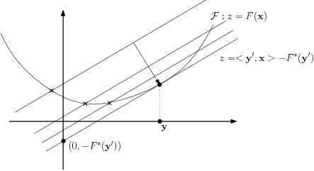
Figure 3: Legendre transformation of a strictly convex function F𝐹F: The z𝑧z-intercept (0,F(𝐲))0superscript𝐹superscript𝐲(0,-F^{*}(\mathbf{y}^{\prime})) of the tangent hyperplane H𝐲:z=𝐲,𝐱F(𝐲):subscript𝐻𝐲𝑧superscript𝐲𝐱superscript𝐹superscript𝐲H_{\mathbf{y}}:z={\langle{\mathbf{y}^{\prime}},{\mathbf{x}}\rangle}-F^{*}(\mathbf{y}^{\prime}) of \mathcal{F} at 𝐲^^𝐲\hat{\mathbf{y}} defines the value of the Legendre transform Fsuperscript𝐹F^{*} for the dual coordinate 𝐲=F(𝐲)superscript𝐲bold-∇𝐹𝐲\mathbf{y}^{\prime}={{\bm{\nabla}}F}(\mathbf{y}). Any hyperplane passing through an other point of \mathcal{F} and parallel to H𝐲subscript𝐻𝐲H_{\mathbf{y}} necessarily intersects the z𝑧z-axis above F(𝐲)superscript𝐹superscript𝐲-F^{*}(\mathbf{y}^{\prime}).

For convenience, we write 𝐱=F(𝐱)superscript𝐱bold-∇𝐹𝐱\mathbf{x}^{\prime}={{\bm{\nabla}}F}(\mathbf{x}) (omitting the F𝐹F in the 𝐱superscript𝐱\mathbf{x}^{\prime} notation as it should be clear from the context). Figure 3 gives a geometric interpretation of the Legendre transformation. Using this notation, Eq. 1 can be rewritten as

DF(𝐩||𝐪)=F(𝐩)F(𝐪)𝐪,𝐩𝐪.D_{F}(\mathbf{p}||\mathbf{q})=F(\mathbf{p})-F(\mathbf{q})-{\langle{\mathbf{q}^{\prime}},{\mathbf{p}-\mathbf{q}}\rangle}. (5)

Since F𝐹F is a strictly convex and differentiable real-valued function on 𝒳𝒳\mathcal{X}, its gradient Fbold-∇𝐹{{\bm{\nabla}}F} is well defined as well as its inverse 1Fsuperscriptbold-∇1𝐹{{\bm{\nabla}^{-1}F}}. Writing 𝒳superscript𝒳\mathcal{X}^{\prime} for the gradient space {F(𝐱)=𝐱|𝐱𝒳}conditional-setbold-∇𝐹𝐱superscript𝐱𝐱𝒳\{{{\bm{\nabla}}F}(\mathbf{x})=\mathbf{x}^{\prime}|\mathbf{x}\in\mathcal{X}\}, the convex conjugate Fsuperscript𝐹F^{*} of F𝐹F is the function: 𝒳dsuperscript𝒳superscript𝑑maps-to\mathcal{X}^{\prime}\subset\mathbb{R}^{d}\mapsto\mathbb{R} defined by

F(𝐱)=𝐱,𝐱F(𝐱).superscript𝐹superscript𝐱𝐱superscript𝐱𝐹𝐱F^{*}(\mathbf{x}^{\prime})={\langle{\mathbf{x}},{\mathbf{x}^{\prime}}\rangle}-F(\mathbf{x}). (6)

Deriving this expression, we get

F(𝐱),d𝐱=𝐱,d𝐱+𝐱,d𝐱F(𝐱),d𝐱=𝐱,d𝐱=1F(𝐱),d𝐱,bold-∇superscript𝐹superscript𝐱dsuperscript𝐱𝐱dsuperscript𝐱superscript𝐱d𝐱bold-∇𝐹𝐱d𝐱𝐱dsuperscript𝐱superscriptbold-∇1𝐹superscript𝐱dsuperscript𝐱{\langle{{{\bm{\nabla}}{F^{*}}}(\mathbf{x}^{\prime})},{\mathrm{d}\mathbf{x}^{\prime}}\rangle}={\langle{\mathbf{x}},{\mathrm{d}\mathbf{x}^{\prime}}\rangle}+{\langle{\mathbf{x}^{\prime}},{\mathrm{d}\mathbf{x}}\rangle}-{\langle{{{\bm{\nabla}}F}(\mathbf{x})},{\mathrm{d}\mathbf{x}}\rangle}={\langle{\mathbf{x}},{\mathrm{d}\mathbf{x}^{\prime}}\rangle}={\langle{{{\bm{\nabla}^{-1}F}}(\mathbf{x}^{\prime})},{\mathrm{d}\mathbf{x}^{\prime}}\rangle},

from which we deduce that F=1Fbold-∇superscript𝐹superscriptbold-∇1𝐹{{\bm{\nabla}}{F^{*}}}={{\bm{\nabla}^{-1}F}}. From Eq. 6, we also deduce (F)=Fsuperscriptsuperscript𝐹𝐹(F^{*})^{*}=F.

From the above discussion, it follows that DFsubscript𝐷superscript𝐹D_{F^{*}} is a Bregman divergence, which we call the Legendre dual divergence of DFsubscript𝐷𝐹D_{F}. We have :

Lemma 3

DF(𝐩||𝐪)=F(𝐩)+F(𝐪)𝐩,𝐪=DF(𝐪||𝐩)D_{F}(\mathbf{p}||\mathbf{q})=F(\mathbf{p})+F^{*}(\mathbf{q}^{\prime})-{\langle{\mathbf{p}},{\mathbf{q}^{\prime}}\rangle}=D_{F^{*}}(\mathbf{q}^{\prime}||\mathbf{p}^{\prime})

Proof: By Eq. 5, DF(𝐩||𝐪)=F(𝐩)F(𝐪)𝐩𝐪,𝐪D_{F}(\mathbf{p}||\mathbf{q})=F(\mathbf{p})-F(\mathbf{q})-{\langle{\mathbf{p}-\mathbf{q}},{\mathbf{q}^{\prime}}\rangle}, and, according to Eq. 6, we have F(𝐩)=𝐩,𝐩F(𝐩)𝐹𝐩superscript𝐩𝐩superscript𝐹superscript𝐩F(\mathbf{p})={\langle{\mathbf{p}^{\prime}},{\mathbf{p}}\rangle}-F^{*}(\mathbf{p}^{\prime}) and F(𝐪)=𝐪,𝐪F(𝐪)𝐹𝐪superscript𝐪𝐪superscript𝐹superscript𝐪F(\mathbf{q})={\langle{\mathbf{q}^{\prime}},{\mathbf{q}}\rangle}-F^{*}(\mathbf{q}^{\prime}). Hence, DF(𝐩||𝐪)=𝐩,𝐩F(𝐩)𝐩,𝐪+F(𝐪)=DF(𝐪||𝐩)D_{F}(\mathbf{p}||\mathbf{q})={\langle{\mathbf{p}^{\prime}},{\mathbf{p}}\rangle}-F^{*}(\mathbf{p}^{\prime})-{\langle{\mathbf{p}},{\mathbf{q}^{\prime}}\rangle}+F^{*}(\mathbf{q}^{\prime})=D_{F^{*}}(\mathbf{q}^{\prime}||\mathbf{p}^{\prime}) since 𝐩=F1F(𝐩)=F(𝐩)𝐩bold-∇superscript𝐹1bold-∇𝐹𝐩bold-∇superscript𝐹superscript𝐩\mathbf{p}={{\bm{\nabla}}F}^{-1}{{\bm{\nabla}}F}(\mathbf{p})={{\bm{\nabla}}F}^{*}(\mathbf{p}^{\prime}). \square

Observe that, when DFsubscript𝐷𝐹D_{F} is symmetric, DFsubscript𝐷superscript𝐹D_{F^{*}} is also symmetric.

The Legendre transform of the quadratic form F(𝐱)=12𝐱T𝐐𝐱𝐹𝐱12superscript𝐱𝑇𝐐𝐱F(\mathbf{x})=\frac{1}{2}\mathbf{x}^{T}\mathbf{Q}\mathbf{x}, where 𝐐𝐐\mathbf{Q} is a symmetric invertible matrix, is F(𝐲)=12𝐲T𝐐1𝐲superscript𝐹𝐲12superscript𝐲𝑇superscript𝐐1𝐲F^{*}(\mathbf{y})=\frac{1}{2}\mathbf{y}^{T}\mathbf{Q}^{-1}\mathbf{y} (corresponding divergences DFsubscript𝐷𝐹D_{F} and DFsubscript𝐷superscript𝐹D_{F^{*}} are both generalized quadratic distances).

To compute Fsuperscript𝐹F^{*}, we use the fact that F=1Fbold-∇superscript𝐹superscriptbold-∇1𝐹{{\bm{\nabla}}{F^{*}}}={{\bm{\nabla}^{-1}F}} and obtain Fsuperscript𝐹F^{*} as F=1Fsuperscript𝐹superscriptbold-∇1𝐹F^{*}=\int{{\bm{\nabla}^{-1}F}}. For example, the Hellinger-like measure is obtained by setting F(x)=1x2𝐹𝑥1superscript𝑥2F(x)=-\sqrt{1-x^{2}} (see Table 1). The inverse gradient is x1+x2𝑥1superscript𝑥2\frac{x}{\sqrt{1+x^{2}}} and the dual convex conjugate is xdx1+x2=1+x2𝑥d𝑥1superscript𝑥21superscript𝑥2\int\frac{x\mathrm{d}x}{\sqrt{1+x^{2}}}=\sqrt{1+x^{2}}. Integrating functions symbolically may be difficult or even not possible, and, in some cases, it will be required to approximate numerically the inverse gradient 1F(𝐱)superscriptbold-∇1𝐹𝐱{{\bm{\nabla}^{-1}F}}(\mathbf{x}).

Let us consider the univariate generator functions defining the divergences of Table 1. Both the squared function F(𝐱)=x2𝐹𝐱superscript𝑥2F(\mathbf{x})=x^{2} and Burg entropy F(x)=logx𝐹𝑥𝑥F(x)=-\log x are self-dual, i.e. F=F𝐹superscript𝐹F=F^{*}. This is easily seen by noticing that the gradient and inverse gradient are identical (up to some constant factor).

For the exponential function F(x)=expx𝐹𝑥𝑥F(x)=\exp x, we have F(y)=ylogyysuperscript𝐹𝑦𝑦𝑦𝑦F^{*}(y)=y\log y-y (the unnormalized Shannon entropy) and for the dual bit entropy F(x)=log(1+expx)𝐹𝑥1𝑥F(x)=\log(1+\exp x), we have F(y)=ylogy1y+log(1y)superscript𝐹𝑦𝑦𝑦1𝑦1𝑦F^{*}(y)=y\log\frac{y}{1-y}+\log(1-y), the bit entropy. Note that the bit entropy function is a particular Bregman generator satisfying F(x)=F(1x)𝐹𝑥𝐹1𝑥F(x)=F(1-x).

2.3 Symmetrized Bregman divergences

For non-symmetric d𝑑d-variate Bregman divergences DFsubscript𝐷𝐹D_{F}, we define the symmetrized divergence

SF(𝐩,𝐪)=SF(𝐪,𝐩)=12(DF(𝐩||𝐪)+DF(𝐪||𝐩))=12𝐩𝐪,𝐩𝐪.S_{F}(\mathbf{p},\mathbf{q})=S_{F}(\mathbf{q},\mathbf{p})=\frac{1}{2}\left(D_{F}(\mathbf{p}||\mathbf{q})+D_{F}(\mathbf{q}||\mathbf{p})\right)=\frac{1}{2}{\langle{\mathbf{p}-\mathbf{q}},{\mathbf{p}^{\prime}-\mathbf{q}^{\prime}}\rangle}.

An example of such a symmetrized divergence is the symmetric Kullback-Leibler divergence (SKL) widely used in computer vision and sound processing (see for example [29]).

A key observation is to note that the divergence SFsubscript𝑆𝐹S_{F} between two points of 𝒳𝒳\mathcal{X} can be measured as a divergence in 𝒳×𝒳2d𝒳superscript𝒳superscript2𝑑\mathcal{X}\times\mathcal{X}^{\prime}\subset\mathbb{R}^{2d}. More precisely, let 𝐱~=[𝐱𝐱]T~𝐱superscriptdelimited-[]𝐱superscript𝐱𝑇{\tilde{\mathbf{x}}}=[\mathbf{x}\ \mathbf{x}^{\prime}]^{T} be the 2d2𝑑2d-dimensional vector obtained by stacking the coordinates of 𝐱𝐱\mathbf{x} on top of those of 𝐱superscript𝐱\mathbf{x}^{\prime}, the gradient of F𝐹F at 𝐱𝐱\mathbf{x}. We have :

Theorem 1

SF(𝐩,𝐪)=12DF~(𝐩~||𝐪~)S_{F}(\mathbf{p},\mathbf{q})=\frac{1}{2}D_{\tilde{F}}(\tilde{\mathbf{p}}||\tilde{\mathbf{q}}) where F~(𝐱~)=F(𝐱)+F(𝐱)~𝐹~𝐱𝐹𝐱superscript𝐹superscript𝐱\tilde{F}(\tilde{\mathbf{x}})=F(\mathbf{x})+F^{*}(\mathbf{x}^{\prime}) and DF~subscript𝐷~𝐹D_{\tilde{F}} is the Bregman divergence defined over 𝒳×𝒳2d𝒳superscript𝒳superscript2𝑑\mathcal{X}\times\mathcal{X}^{\prime}\subset\mathbb{R}^{2d} for the generator function F~~𝐹\tilde{F}.

Proof: Using Lemma 3, we have

SF(𝐩,𝐪)=12(DF(𝐩||𝐪)+DF(𝐪||𝐩))=12(DF(𝐩||𝐪)+DF(𝐩||𝐪))=12DF~(𝐩~||𝐪~)S_{F}(\mathbf{p},\mathbf{q})=\frac{1}{2}\left(D_{F}(\mathbf{p}||\mathbf{q})+D_{F}(\mathbf{q}||\mathbf{p})\right)=\frac{1}{2}\left(D_{F}(\mathbf{p}||\mathbf{q})+D_{F^{*}}(\mathbf{p}^{\prime}||\mathbf{q}^{\prime})\right)=\frac{1}{2}D_{\tilde{F}}(\tilde{\mathbf{p}}||\tilde{\mathbf{q}})

\square

It should be noted that 𝐱~~𝐱\tilde{\mathbf{x}} lies on the d𝑑d-manifold 𝒳~={[𝐱𝐱]T|𝐱d}~𝒳conditional-setsuperscriptdelimited-[]𝐱superscript𝐱𝑇𝐱superscript𝑑\tilde{\mathcal{X}}=\{[\mathbf{x}\ \mathbf{x}^{\prime}]^{T}\ |\ \mathbf{x}\in\mathbb{R}^{d}\} of 2dsuperscript2𝑑\mathbb{R}^{2d}. Note also that SF(𝐩,𝐪)subscript𝑆𝐹𝐩𝐪S_{F}(\mathbf{p},\mathbf{q}) is symmetric but not a Bregman divergence in general since 𝒳~~𝒳\tilde{\mathcal{X}} may not be convex, while DF~subscript𝐷~𝐹D_{\tilde{F}} is a non symmetric Bregman divergence in 𝒳×𝒳𝒳superscript𝒳\mathcal{X}\times\mathcal{X}^{\prime}.

2.4 Exponential families

2.4.1 Parametric statistical spaces and exponential families

A statistical space 𝒳𝒳\mathcal{X} is an abstract space where coordinates of vector points 𝜽𝒳𝜽𝒳{\bm{\theta}}\in\mathcal{X} encode the parameters of statistical distributions. The dimension d=dim𝒳𝑑dimension𝒳d=\dim\mathcal{X} of the statistical space coincides with the finite number of free parameters of the distribution laws. For example, the space 𝒳={[μσ]T|(μ,σ)×+}𝒳conditional-setsuperscriptdelimited-[]𝜇𝜎𝑇𝜇𝜎subscriptsuperscript\mathcal{X}=\{[\mu\ \sigma]^{T}\ |\ (\mu,\sigma)\in\mathbb{R}\times\mathbb{R}^{+}_{*}\} of univariate normal distributions 𝒩(μ,σ)𝒩𝜇𝜎\mathcal{N}(\mu,\sigma) is a 2D parametric statistical space, extensively studied in information geometry [1] under the auspices of differential geometry. A prominent class of distribution families called the exponential families Fsubscript𝐹\mathcal{E}_{F} [1] admits the same canonical probability distribution function

p(x|𝜽)=defexp{𝜽,𝐟(x)F(𝜽)+C(x)},superscriptdef𝑝conditional𝑥𝜽𝜽𝐟𝑥𝐹𝜽𝐶𝑥p(x|{\bm{\theta}})\stackrel{{\scriptstyle\mathrm{def}}}{{=}}\exp\{{\langle{{\bm{\theta}}},{\mathbf{f}(x)}\rangle}-F({\bm{\theta}})+C(x)\}, (7)

where 𝐟(x)𝐟𝑥\mathbf{f}(x) denotes the sufficient statistics and 𝜽𝒳𝜽𝒳{\bm{\theta}}\in\mathcal{X} represents the natural parameters. Space 𝒳𝒳\mathcal{X} is thus called the natural parameter space and, since logxp(x|𝜽)dx=log1=0subscript𝑥𝑝conditional𝑥𝜽differential-d𝑥10\log\int_{x}p(x|{\bm{\theta}})\mathrm{d}x=\log 1=0, we have F(𝜽)=logxexp{𝜽,𝐟(𝐱)+C(x)}dx𝐹𝜽subscript𝑥𝜽𝐟𝐱𝐶𝑥differential-d𝑥F({\bm{\theta}})=\log\int_{x}\exp\{{\langle{{\bm{\theta}}},{\mathbf{f}(\mathbf{x})}\rangle}+C(x)\}\mathrm{d}x. F𝐹F is called the cumulant function or the log-partition function. F𝐹F fully characterizes the exponential family Fsubscript𝐹\mathcal{E}_{F} while term C(x)𝐶𝑥C(x) ensures density normalization. (That is, p(x|𝜽)𝑝conditional𝑥𝜽p(x|{\bm{\theta}}) is indeed a probability density function satisfying xp(x|𝜽)dx=1subscript𝑥𝑝conditional𝑥𝜽differential-d𝑥1\int_{x}p(x|{\bm{\theta}})\mathrm{d}x=1.)

Exponential familyCanonical probability density function:exp{𝜽,𝐟(x)F(𝜽)+C(x)}NaturalSufficientCumulant functionF(𝜽)Dens. Norm.parameters𝜽statistics𝐟(x)C(x)Bernouilli (q) (Tossing coin with Pr(heads)=q and Pr(tails)=1qlogq1qxlog(1+expθ)0 Multinomial (q1,,qd+1) (Extend Bernouilli with Pr(xi)=qi and iqi=1)θi=logqi1j=1dqifi(𝐱)=xilog(1+i=1dexpθi)0Beta β(θ1,θ2) (Bernouilli conjugate prior) [θ1θ2]T[logxlog(1x)]TlogB(θ1+1,θ2+1)0F(𝜽)=logΓ(θ1+1)Γ(θ2+1)Γ(θ1+θ22)(withΓ(x)=0tx1exp(t)dt)=(x1)Γ(x1))Univariate Normal 𝒩(μ,σ2)[μσ212σ2]T[xx2]Tθ124θ2+12log(πθ2)0Multivariate Normal 𝒩(𝝁,𝚺) [𝚺1𝝁12𝚺1][𝐱𝐱𝐱T]12𝝁T𝚺1𝝁+12logdet(2π𝚺)0Rayleigh (σ2) (used in ultrasound imageries)12σ2x2log12θlogxLaplacian (θ) (used in radioactivity decay) θxlogθ0Poisson 𝒫(λ) (counting process) logλxexpθlogx!Gamma γ(θ1,θ2) (waiting times in Poisson processes)[θ1θ2]T[logxx]TlogΓ(θ1+1)+(θ2+1)log(θ2)0Dirichlet 𝒟(𝜶) (varying proportion model 𝐱=1, conjugate prior of Multinomial)θi=αi1fi(𝐱)=logxilogΓ(iθi+d)iΓ(θi+1)0\begin{array}[]{|l|l|l|l|}\hline\cr\vrule\lx@intercol\hfil\mbox{\large Exponential family}\hfil\lx@intercol\vrule\lx@intercol\\ \vrule\lx@intercol\hfil\mbox{Canonical probability density function:}\exp\{{\langle{{\bm{\theta}}},{\mathbf{f}(x)}\rangle}-F({\bm{\theta}})+C(x)\}\hfil\lx@intercol\vrule\lx@intercol\\ \hline\cr\hline\cr\hline\cr\mbox{Natural}&\mbox{Sufficient}&\mbox{Cumulant function}\ F({\bm{\theta}})&\mbox{Dens. Norm.}\\ \mbox{parameters}\ {\bm{\theta}}&\mbox{statistics}\ \mathbf{f}(x)&&C(x)\\ \hline\cr\hline\cr\vrule\lx@intercol\hfil\mbox{Bernouilli $\mathcal{B}(q)$ (Tossing coin with $\Pr(\mathrm{heads})=q$ and $\Pr(\mathrm{tails})=1-q$) }\hfil\lx@intercol\vrule\lx@intercol\\ \hline\cr\log\frac{q}{1-q}&x&\log(1+\exp\theta)&0\\ \hline\cr\hline\cr\vrule\lx@intercol\hfil\mbox{ Multinomial $\mathcal{M}(q_{1},...,q_{d+1})$ (Extend Bernouilli with $\Pr(x_{i})=q_{i}$ and $\sum_{i}q_{i}=1$)}\hfil\lx@intercol\vrule\lx@intercol\\ \hline\cr\theta_{i}=\log\frac{q_{i}}{1-\sum_{j=1}^{d}q_{i}}&f_{i}(\mathbf{x})=x_{i}&\log(1+\sum_{i=1}^{d}\exp\theta_{i})&0\\ \hline\cr\vrule\lx@intercol\hfil\mbox{Beta $\beta(\theta_{1},\theta_{2})$ (Bernouilli conjugate prior) }\hfil\lx@intercol\vrule\lx@intercol\\ \hline\cr[\theta_{1}\ \theta_{2}]^{T}&[\log x\ \log(1-x)]^{T}&\log B(\theta_{1}+1,\theta_{2}+1)&0\\ \hline\cr\vrule\lx@intercol\hfil F({\bm{\theta}})=\log\frac{\Gamma(\theta_{1}+1)\Gamma(\theta_{2}+1)}{\Gamma(\theta_{1}+\theta_{2}-2)}\hfil\lx@intercol\vrule\lx@intercol\\ \vrule\lx@intercol\hfil(\mbox{with}\ \Gamma(x)=\int_{0}^{\infty}t^{x-1}\exp(-t)\mathrm{d}t)=(x-1)\Gamma(x-1))\hfil\lx@intercol\vrule\lx@intercol\\ \hline\cr\hline\cr\vrule\lx@intercol\hfil\mbox{Univariate Normal $\mathcal{N}(\mu,\sigma^{2})$}\hfil\lx@intercol\vrule\lx@intercol\\ \hline\cr[\frac{\mu}{\sigma^{2}}\ \frac{-1}{2\sigma^{2}}]^{T}&[x\ x^{2}]^{T}&-\frac{\theta_{1}^{2}}{4\theta_{2}}+\frac{1}{2}\log(-\frac{\pi}{\theta_{2}})&0\\ \hline\cr\hline\cr\vrule\lx@intercol\hfil\mbox{Multivariate Normal $\mathcal{N}({\bm{\mu}},{\bm{\Sigma}})$ }\hfil\lx@intercol\vrule\lx@intercol\\ \hline\cr[{\bm{\Sigma}}^{-1}{\bm{\mu}}\ -\frac{1}{2}{\bm{\Sigma}}^{-1}]&[\mathbf{x}\ \mathbf{x}\mathbf{x}^{T}]&\frac{1}{2}{\bm{\mu}}^{T}{\bm{\Sigma}}^{-1}{\bm{\mu}}+\frac{1}{2}\log\det(2\pi{\bm{\Sigma}})&0\\ \hline\cr\hline\cr\vrule\lx@intercol\hfil\mbox{Rayleigh $\mathcal{R}(\sigma^{2})$ (used in ultrasound imageries)}\hfil\lx@intercol\vrule\lx@intercol\\ \hline\cr-\frac{1}{2\sigma^{2}}&x^{2}&\log-\frac{1}{2\theta}&\log x\\ \hline\cr\hline\cr\vrule\lx@intercol\hfil\mbox{Laplacian $\mathcal{L}(\theta)$ (used in radioactivity decay) }\hfil\lx@intercol\vrule\lx@intercol\\ \hline\cr\theta&-x&-\log\theta&0\\ \hline\cr\hline\cr\vrule\lx@intercol\hfil\mbox{Poisson $\mathcal{P}(\lambda)$ (counting process) }\hfil\lx@intercol\vrule\lx@intercol\\ \hline\cr\log\lambda&x&\exp\theta&-\log x!\\ \hline\cr\hline\cr\vrule\lx@intercol\hfil\mbox{Gamma $\gamma(\theta_{1},\theta_{2})$ (waiting times in Poisson processes)}\hfil\lx@intercol\vrule\lx@intercol\\ \hline\cr[\theta_{1}\ \theta_{2}]^{T}&[\log x\ x]^{T}&\log\Gamma(\theta_{1}+1)+(\theta_{2}+1)\log(-\theta_{2})&0\\ \hline\cr\hline\cr\vrule\lx@intercol\hfil\mbox{Dirichlet $\mathcal{D}({\bm{\alpha}})$ (varying proportion model $||\mathbf{x}||=1$, conjugate prior of Multinomial)}\hfil\lx@intercol\vrule\lx@intercol\\ \hline\cr\theta_{i}=\alpha_{i}-1&f_{i}(\mathbf{x})=\log x_{i}&\log\Gamma(\sum_{i}\theta_{i}+d)-\sum_{i}\Gamma(\theta_{i}+1)&0\\ \hline\cr\end{array}
Table 2: Canonical decompositions of usual exponential families.

When the components of the sufficient statistics are affinely independent, this canonical representation is said to be minimal, and the family Fsubscript𝐹\mathcal{E}_{F} is called a full exponential family of order d=dim𝒳𝑑dimension𝒳d=\dim\mathcal{X}. Moreover, we consider regular exponential families Fsubscript𝐹\mathcal{E}_{F} that have their support domains topologically open. Regular exponential families include many famous distribution laws such as Bernoulli (multinomial), Normal (univariate, multivariate and rectified), Poisson, Laplacian, negative binomial, Rayleigh, Wishart, Dirichlet, and Gamma distributions. Table 2 summarizes the various relevant parts of the canonical decompositions of some of these usual statistical distributions. Observe that the product of any two distributions of the same exponential family is another exponential family distribution that may not have anymore a nice parametric form (except for products of normal distribution pdfs that yield again normal distribution pdfs). Thus exponential families provide a unified treatment framework of common distributions. Note, however, that the uniform distribution does not belong to the exponential families.

2.4.2 Kullback-Leibler divergence of exponential families

In such statistical spaces 𝒳𝒳\mathcal{X}, a basic primitive is to measure the distortion between any two distributions. The Kullback-Leibler divergence (also called relative entropy or information divergence, I𝐼I-divergence) is a standard information-theoretic measure between two statistical distributions d1subscript𝑑1d_{1} and d2subscript𝑑2d_{2} defined as KL(d1||d2)=defxd1(x)logd1(x)d2(x)dx\mathrm{KL}(d_{1}||d_{2})\stackrel{{\scriptstyle\mathrm{def}}}{{=}}\int_{x}d_{1}(x)\log\frac{d_{1}(x)}{d_{2}(x)}\mathrm{d}x. This statistical measure is not symmetric nor does the triangle inequality holds.

The link with Bregman divergences comes from the remarkable property that the Kullback-Leibler divergence of any two distributions of the same exponential family with respective natural parameters 𝜽psubscript𝜽𝑝{\bm{\theta}}_{p} and 𝜽qsubscript𝜽𝑞{\bm{\theta}}_{q} is obtained from the Bregman divergence induced by the cumulant function of that family by swapping arguments. By a slight abuse of notations, we denote by KL(𝜽p||𝜽q)\mathrm{KL}({\bm{\theta}}_{p}||{\bm{\theta}}_{q}) the oriented Kullback-Leibler divergence between the probability density functions defined by the respective natural parameters, i.e. KL(𝜽p||𝜽q)=defxp(x|𝜽p)logp(x|𝜽p)p(x|𝜽q)dx\mathrm{KL}({\bm{\theta}}_{p}||{\bm{\theta}}_{q})\stackrel{{\scriptstyle\mathrm{def}}}{{=}}\int_{x}p(x|{\bm{\theta}}_{p})\log\frac{p(x|{\bm{\theta}}_{p})}{p(x|{\bm{\theta}}_{q})}\mathrm{d}x. The following theorem is the extension to the continuous case of a result mentioned in  [6].

Theorem 2

The Kullback-Leibler divergence of any two distributions of the same exponential family with natural parameters 𝛉psubscript𝛉𝑝{\bm{\theta}}_{p} and 𝛉qsubscript𝛉𝑞{\bm{\theta}}_{q} is obtained from the Bregman divergence induced by the cumulant function F𝐹F as: KL(𝛉p||𝛉q)=DF(𝛉q||𝛉p)\mathrm{KL}({\bm{\theta}}_{p}||{\bm{\theta}}_{q})=D_{F}({\bm{\theta}}_{q}||{\bm{\theta}}_{p}).

Before proving the theorem, we note that

F(𝜽)=[x𝐟(x)exp{𝜽,𝐟(x)F(𝜽)+C(x)}dx].bold-∇𝐹𝜽delimited-[]subscript𝑥𝐟𝑥𝜽𝐟𝑥𝐹𝜽𝐶𝑥differential-d𝑥\bm{\nabla}F({\bm{\theta}})=\left[\int_{x}\mathbf{f}(x)\exp\{{\langle{{\bm{\theta}}},{\mathbf{f}(x)}\rangle}-F({\bm{\theta}})+C(x)\}\mathrm{d}x\right]. (8)

The coordinates of 𝝁=defF(𝜽)=[x𝐟(𝐱)p(x|𝜽)dx]=E𝜽(𝐟(𝐱))superscriptdef𝝁bold-∇𝐹𝜽delimited-[]subscript𝑥𝐟𝐱𝑝conditional𝑥𝜽differential-d𝑥subscript𝐸𝜽𝐟𝐱{\bm{\mu}}\stackrel{{\scriptstyle\mathrm{def}}}{{=}}\bm{\nabla}F({\bm{\theta}})=[\int_{x}\mathbf{f}(\mathbf{x})p(x|{\bm{\theta}})\mathrm{d}x]=E_{{\bm{\theta}}}(\mathbf{f}(\mathbf{x})) are called the expectation parameters. As an example, consider the univariate normal distribution 𝒩(μ,σ)𝒩𝜇𝜎\mathcal{N}(\mu,\sigma) with sufficient statistics [xx2]Tsuperscriptdelimited-[]𝑥superscript𝑥2𝑇[x\ x^{2}]^{T} (see Table 2). The expectation parameters are 𝝁=F(𝜽)=[μμ2+σ2]T𝝁subscriptbold-∇𝐹𝜽superscriptdelimited-[]𝜇superscript𝜇2superscript𝜎2𝑇{\bm{\mu}}=\bm{\nabla}_{F}({\bm{\theta}})=[\mu\ \mu^{2}+\sigma^{2}]^{T}, where μ=xxp(x|𝜽)dx𝜇subscript𝑥𝑥𝑝conditional𝑥𝜽differential-d𝑥\mu=\int_{x}x\,p(x|{\bm{\theta}})\mathrm{d}x and μ2+σ2=xx2p(x|𝜽)dxsuperscript𝜇2superscript𝜎2subscript𝑥superscript𝑥2𝑝conditional𝑥𝜽differential-d𝑥\mu^{2}+\sigma^{2}=\int_{x}x^{2}p(x|{\bm{\theta}})\mathrm{d}x.

We now prove the theorem.

Proof:

KL(𝜽p||𝜽q)\displaystyle\mathrm{KL}({\bm{\theta}}_{p}||{\bm{\theta}}_{q}) =\displaystyle= xp(x|𝜽p)logp(x|𝜽p)p(x|𝜽q)dxsubscript𝑥𝑝conditional𝑥subscript𝜽𝑝𝑝conditional𝑥subscript𝜽𝑝𝑝conditional𝑥subscript𝜽𝑞d𝑥\displaystyle\int_{x}p(x|{\bm{\theta}}_{p})\log\frac{p(x|{\bm{\theta}}_{p})}{p(x|{\bm{\theta}}_{q})}\mathrm{d}x
=\displaystyle= xp(x|𝜽p)(F(𝜽q)F(𝜽p)+𝜽p𝜽q,𝐟(x))dxsubscript𝑥𝑝conditional𝑥subscript𝜽𝑝𝐹subscript𝜽𝑞𝐹subscript𝜽𝑝subscript𝜽𝑝subscript𝜽𝑞𝐟𝑥differential-d𝑥\displaystyle\int_{x}p(x|{\bm{\theta}}_{p})(F({\bm{\theta}}_{q})-F({\bm{\theta}}_{p})+{\langle{{\bm{\theta}}_{p}-{\bm{\theta}}_{q}},{\mathbf{f}(x)}\rangle})\mathrm{d}x
=\displaystyle= xp(x|𝜽p)(DF(𝜽q||𝜽p)+𝜽q𝜽p,F(𝜽p)+𝜽p𝜽q,𝐟(x))dx\displaystyle\int_{x}p(x|{\bm{\theta}}_{p})\left(D_{F}({\bm{\theta}}_{q}||{\bm{\theta}}_{p})+{\langle{{\bm{\theta}}_{{q}}-{\bm{\theta}}_{{p}}},{{{\bm{\nabla}}F}({\bm{\theta}}_{p})}\rangle}+{\langle{{\bm{\theta}}_{p}-{\bm{\theta}}_{q}},{\mathbf{f}(x)}\rangle}\right)\mathrm{d}x
=\displaystyle= DF(𝜽q||𝜽p)+xp(x|𝜽p)𝜽q𝜽p,F(𝜽p)𝐟(x))dx\displaystyle D_{F}({\bm{\theta}}_{q}||{\bm{\theta}}_{p})+\int_{x}p(x|{\bm{\theta}}_{p}){\langle{{\bm{\theta}}_{q}-{\bm{\theta}}_{p}},{{{\bm{\nabla}}F}({\bm{\theta}}_{p})-\mathbf{f}(x)}\rangle})\mathrm{d}x
=\displaystyle= DF(𝜽q||𝜽p)xp(x|𝜽p)𝜽q𝜽p,𝐟(x)dx+𝜽q𝜽p,F(𝜽p)\displaystyle D_{F}({\bm{\theta}}_{q}||{\bm{\theta}}_{p})-\int_{x}p(x|{\bm{\theta}}_{p}){\langle{{\bm{\theta}}_{q}-{\bm{\theta}}_{p}},{\mathbf{f}(x)}\rangle}\mathrm{d}x+{\langle{{\bm{\theta}}_{q}-{\bm{\theta}}_{p}},{{{\bm{\nabla}}F}({\bm{\theta}}_{p})}\rangle}
=(Eq.8)superscriptformulae-sequenceEq8\displaystyle\stackrel{{\scriptstyle({\rm Eq.}~{}\ref{eq-expo-grad})}}{{=}} DF(𝜽q||𝜽p)\displaystyle D_{F}({\bm{\theta}}_{q}||{\bm{\theta}}_{p})

\square

2.4.3 Dual parameterizations and dual divergences

The notion of dual Bregman divergences introduced earlier and dual parameterizations extend naturally to statistical spaces. Since, 𝝁=F(𝜽)𝝁bold-∇𝐹𝜽{\bm{\mu}}=\bm{\nabla}F({\bm{\theta}}) (Eq. 8), the convex conjugate of F(𝜽)𝐹𝜽F({\bm{\theta}}) is F(𝝁)=𝜽,𝝁F(𝜽)superscript𝐹𝝁𝜽𝝁𝐹𝜽F^{*}({\bm{\mu}})={\langle{{\bm{\theta}}},{{\bm{\mu}}}\rangle}-F({\bm{\theta}}) (Eq. 6). From Lemma 3, we then deduce the following theorem.

Theorem 3

DF(𝜽p||𝜽q)=DF(𝝁q||𝝁p)D_{F}({\bm{\theta}}_{p}||{\bm{\theta}}_{q})=D_{F^{*}}({\bm{\mu}}_{q}||{\bm{\mu}}_{p}) where Fsuperscript𝐹F^{*} denote the convex conjugate of F𝐹F.

Table 3 presents some examples of dual parameterizations of exponential families (i.e., the natural 𝜽𝜽{\bm{\theta}}-parameters and expectation 𝝁𝝁{\bm{\mu}}-parameters and dual Legendre cumulant functions), and describe the corresponding Bregman divergences induced by the Kullback-Leibler divergences.

Bernouilli dual divergences: Logistic loss/binary relative entropyF(θ)=log(1+expθ)DF(θ||θ)=log1+expθ1+expθ(θθ)expθ1+expθf(θ)=expθ1+expθ=μF(μ)=μlogμ+(1μ)log(1μ)DF(μ||μ)=μlogμμ+(1μ)log1μ1μf(μ)=logμ1μ=θPoisson dual divergences: Exponential loss/Unnormalized Shannon entropyF(θ)=expθDF(θ||θ)=expθexpθ(θθ)expθf(θ)=expθ=μF(μ)=μlogμμDF(μ||μ)=μlogμμ+μμf(μ)=logμ=θ\begin{array}[]{|l|l|l|}\hline\cr\vrule\lx@intercol\hfil\mbox{Bernouilli dual divergences: Logistic loss/binary relative entropy}\hfil\lx@intercol\vrule\lx@intercol\\ \hline\cr F(\theta)=\log(1+\exp\theta)&D_{F}(\theta||\theta^{\prime})=\log\frac{1+\exp\theta}{1+\exp\theta^{\prime}}-(\theta-\theta^{\prime})\frac{\exp\theta^{\prime}}{1+\exp\theta^{\prime}}&f(\theta)=\frac{\exp\theta}{1+\exp\theta}=\mu\\ \hline\cr F^{*}(\mu)=\mu\log\mu+(1-\mu)\log(1-\mu)&D_{F^{*}}(\mu^{\prime}||\mu)=\mu^{\prime}\log\frac{\mu^{\prime}}{\mu}+(1-\mu)\log\frac{1-\mu^{\prime}}{1-\mu}&f^{*}(\mu)=\log\frac{\mu}{1-\mu}=\theta\\ \hline\cr\hline\cr\vrule\lx@intercol\hfil\mbox{Poisson dual divergences: Exponential loss/Unnormalized Shannon entropy}\hfil\lx@intercol\vrule\lx@intercol\\ \hline\cr F(\theta)=\exp\theta&D_{F}(\theta||\theta^{\prime})=\exp\theta-\exp\theta^{\prime}-(\theta-\theta^{\prime})\exp\theta^{\prime}&f(\theta)=\exp\theta=\mu\\ \hline\cr F^{*}(\mu)=\mu\log\mu-\mu&D_{F^{*}}(\mu^{\prime}||\mu)=\mu^{\prime}\log\frac{\mu^{\prime}}{\mu}+\mu-\mu^{\prime}&f^{*}(\mu)=\log\mu=\theta\\ \hline\cr\end{array}
Table 3: Examples of dual parameterizations of exponential families and their corresponding Kullback-Leibler (Bregman) divergences for the Bernoulli and Poisson distributions.

Finally, we would like to point out that Banerjee et al. [6] have shown that there is a bijection between the regular exponential families and a subset of the Bregman divergences called regular Bregman divergences.

3 Elements of Bregman geometry

In this section, we discuss several basic geometric properties that will be useful when studying Bregman Voronoi diagrams. Specifically, we characterize Bregman bisectors, Bregman balls and Bregman geodesics. Since Bregman divergences are not symmetric, we describe several types of Bregman bisectors in §3.1. We subsequently characterize Bregman balls by using a lifting transform that extends a construction well-known in the Euclidean case (§3.2). Finally, we characterize geodesics and show an orthogonality property between bisectors and geodesics in §3.3.

3.1 Bregman bisectors

Since Bregman divergences are not symmetric, we can define several types of bisectors. The Bregman bisector of the first type is defined as

HF(𝐩,𝐪)={𝐱𝒳|DF(𝐱||𝐩)=DF(𝐱||𝐪)}.H_{F}({\mathbf{p}},{\mathbf{q}})=\{\mathbf{x}\in\mathcal{X}\ |\ D_{F}(\mathbf{x}||\mathbf{p})=D_{F}(\mathbf{x}||\mathbf{q})\}.

Similarly, we define the Bregman bisector of the second type as

HF(𝐩,𝐪)={𝐱𝒳|DF(𝐩||𝐱)=DF(𝐪||𝐱)}.H^{\prime}_{F}({\mathbf{p}},{\mathbf{q}})=\{\mathbf{x}\in\mathcal{X}\ |\ D_{F}(\mathbf{p}||\mathbf{x})=D_{F}(\mathbf{q}||\mathbf{x})\}.

These bisectors are identical when the divergence is symmetric. However, in general, they are distinct, the bisectors of the first type being linear while the bisectors of the second type are potentially curved (but always linear in the gradient space, hence the notation). More precisely, we have the following lemma

Lemma 4

The Bregman bisector of the first type HF(𝐩,𝐪)subscript𝐻𝐹𝐩𝐪H_{F}(\mathbf{p},\mathbf{q}) is the hyperplane of equation:

HF(𝐩,𝐪):𝐱,𝐩𝐪+F(𝐩)𝐩,𝐩F(𝐪)+𝐪,𝐪=0:subscript𝐻𝐹𝐩𝐪𝐱superscript𝐩superscript𝐪𝐹𝐩𝐩superscript𝐩𝐹𝐪𝐪superscript𝐪0H_{F}({\mathbf{p}},{\mathbf{q}}):{\langle{\mathbf{x}},{\mathbf{p}^{\prime}-\mathbf{q}^{\prime}}\rangle}+F(\mathbf{p})-{\langle{\mathbf{p}},{\mathbf{p}^{\prime}}\rangle}-F(\mathbf{q})+{\langle{\mathbf{q}},{\mathbf{q}^{\prime}}\rangle}=0\

The Bregman bisector of the second type HF(𝐩,𝐪)subscriptsuperscript𝐻𝐹𝐩𝐪H^{\prime}_{F}(\mathbf{p},\mathbf{q}) is the hypersurface of equation

HF(𝐩,𝐪):𝐱,𝐪𝐩+F(𝐩)F(𝐪)=0:subscriptsuperscript𝐻𝐹𝐩𝐪superscript𝐱𝐪𝐩𝐹𝐩𝐹𝐪0H^{\prime}_{F}(\mathbf{p},\mathbf{q}):{\langle{\mathbf{x}^{\prime}},{\mathbf{q}-\mathbf{p}}\rangle}+F(\mathbf{p})-F(\mathbf{q})=0

(a hyperplane in the gradient space 𝒳superscript𝒳\mathcal{X}^{\prime}).

It should be noted that 𝐩𝐩\mathbf{p} and 𝐪𝐪\mathbf{q} lie necessarily on different sides of HF(𝐩,𝐪)subscript𝐻𝐹𝐩𝐪H_{F}(\mathbf{p},\mathbf{q}) since HF(𝐩,𝐪)(𝐩)=DF(𝐩||𝐪)<0H_{F}(\mathbf{p},\mathbf{q})(\mathbf{p})=-D_{F}(\mathbf{p}||\mathbf{q})<0 and HF(𝐩,𝐪)(𝐪)=DF(𝐪||𝐩)>0H_{F}(\mathbf{p},\mathbf{q})(\mathbf{q})=D_{F}(\mathbf{q}||\mathbf{p})>0.

From Lemma 3, we know that DF(𝐱||𝐲)=DF(𝐲||𝐱)D_{F}(\mathbf{x}||\mathbf{y})=D_{F^{*}}(\mathbf{y}^{\prime}||\mathbf{x}^{\prime}) where Fsuperscript𝐹F^{*} is the convex conjugate of F𝐹F. We therefore have

HF(𝐩,𝐪)subscript𝐻𝐹𝐩𝐪\displaystyle H_{F}({\mathbf{p}},{\mathbf{q}}) =\displaystyle= 1F(HF(𝐪,𝐩)),superscriptbold-∇1𝐹subscriptsuperscript𝐻superscript𝐹superscript𝐪superscript𝐩\displaystyle{{\bm{\nabla}^{-1}F}}(H^{\prime}_{F^{*}}({\mathbf{q}^{\prime}},{\mathbf{p}^{\prime}})),
HF(𝐩,𝐪)subscriptsuperscript𝐻𝐹𝐩𝐪\displaystyle H^{\prime}_{F}({\mathbf{p}},{\mathbf{q}}) =\displaystyle= 1F(HF(𝐪,𝐩)).superscriptbold-∇1𝐹subscript𝐻superscript𝐹superscript𝐪superscript𝐩\displaystyle{{\bm{\nabla}^{-1}F}}(H_{F^{*}}({\mathbf{q}^{\prime}},{\mathbf{p}^{\prime}})).

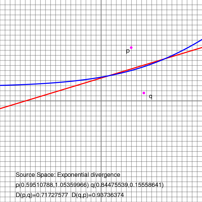
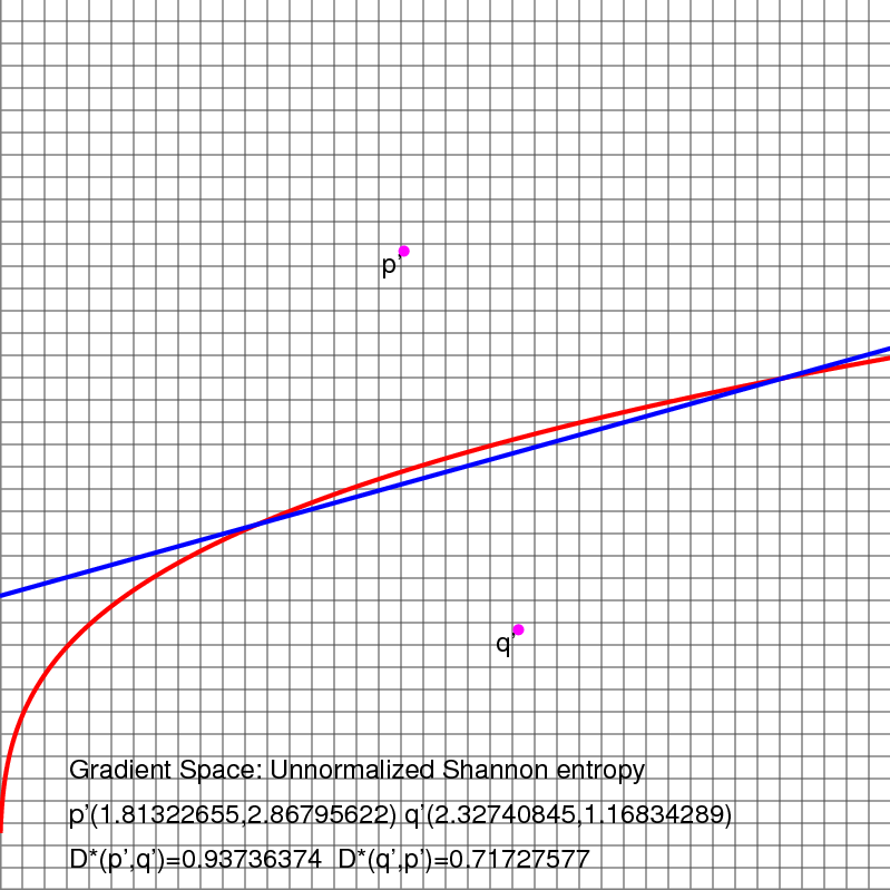
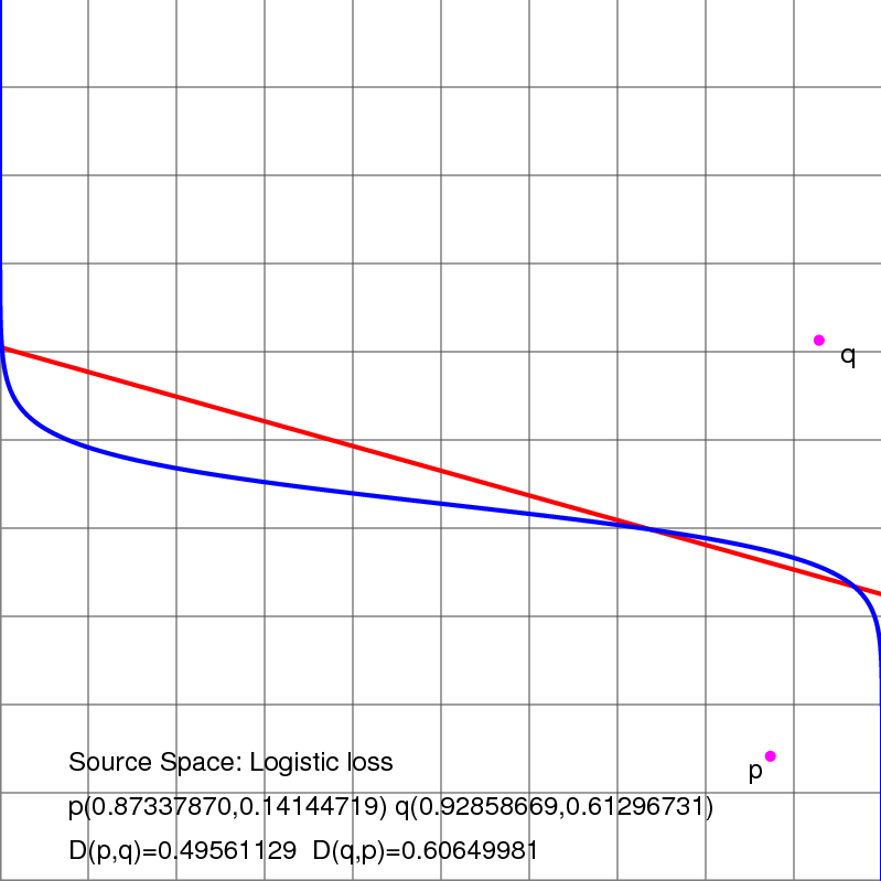
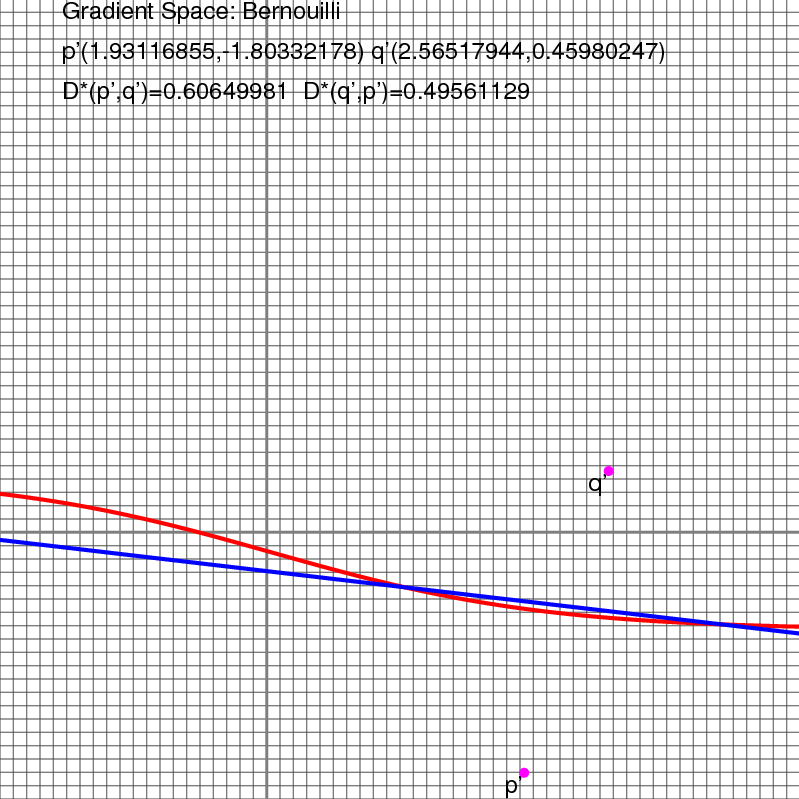
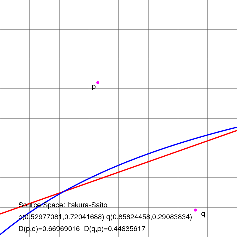
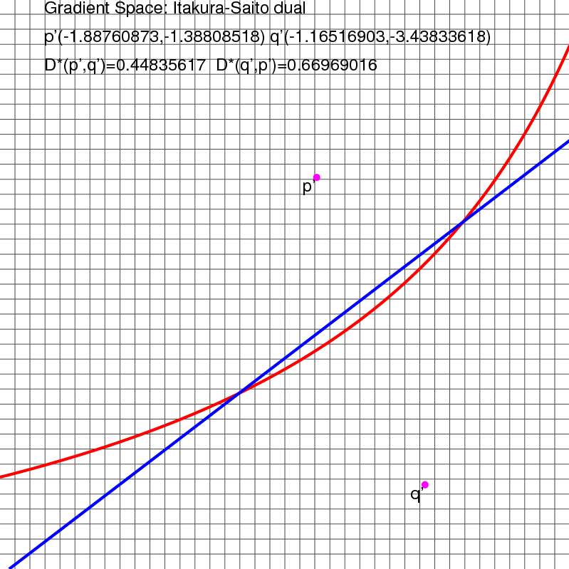
Figure 4 depicts several first-type and second-type bisectors for various pairs of primal/dual Bregman divergences.

Source space 𝒳𝒳\mathcal{X} Gradient space 𝒳superscript𝒳\mathcal{X}^{\prime}
(a) Refer to caption Refer to caption
(b) Refer to caption Refer to caption
(c) Refer to caption Refer to caption
Figure 4: Bregman bisectors: first-type linear bisector and second-type curved bisector are displayed for pairs of primal/dual Bregman divergences: (a) exponential loss/unnormalized Shannon entropy, (b) logistic loss/dual logistic loss, and (c) self-dual Itakura-Saito divergence. The grid size of 2superscript2\mathbb{R}^{2} in 𝒳𝒳\mathcal{X} and 𝒳superscript𝒳\mathcal{X}^{\prime} is ten ticks per unit. First-type (primal linear/dual curved) and second-type (primal curved/dual linear) bisectors are respectively drawn in red and blue.

The bisector HF′′(𝐩,𝐪)subscriptsuperscript𝐻′′𝐹𝐩𝐪H^{{}^{\prime\prime}}_{F}(\mathbf{p},\mathbf{q}) for the symmetrized Bregman divergence SFsubscript𝑆𝐹S_{F} is given by

HF′′(𝐩,𝐪):𝐱,𝐪𝐩+𝐱,𝐪𝐩+𝐩,𝐩𝐪,𝐪=0.:subscriptsuperscript𝐻′′𝐹𝐩𝐪𝐱superscript𝐪superscript𝐩superscript𝐱𝐪𝐩𝐩superscript𝐩𝐪superscript𝐪0H^{{}^{\prime\prime}}_{F}({\mathbf{p}},{\mathbf{q}}):{\langle{\mathbf{x}},{\mathbf{q}^{\prime}-\mathbf{p}^{\prime}}\rangle}+{\langle{\mathbf{x}^{\prime}},{\mathbf{q}-\mathbf{p}}\rangle}+{\langle{\mathbf{p}},{\mathbf{p}^{\prime}}\rangle}-{\langle{\mathbf{q}},{\mathbf{q}^{\prime}}\rangle}=0.

Such a bisector is not linear in 𝐱𝐱\mathbf{x} nor in 𝐱superscript𝐱\mathbf{x}^{\prime}. However, we can observe that the expression is linear in 𝐱~=[𝐱𝐱]T~𝐱superscriptdelimited-[]𝐱superscript𝐱𝑇\tilde{\mathbf{x}}=[\mathbf{x}\ \mathbf{x}^{\prime}]^{T}. Indeed, proceeding as we did in §2.3, we can rewrite the above equation as

HF~(𝐩~,𝐪~):[𝐱𝐱],[𝐪𝐩𝐪𝐩]+𝐩,𝐩𝐪,𝐪=0.:subscript𝐻~𝐹~𝐩~𝐪delimited-[]𝐱superscript𝐱delimited-[]superscript𝐪superscript𝐩𝐪𝐩𝐩superscript𝐩𝐪superscript𝐪0H_{\tilde{F}}(\tilde{\mathbf{p}},\tilde{\mathbf{q}}):{\left\langle{\left[\begin{array}[]{c}\mathbf{x}\\ \mathbf{x}^{\prime}\end{array}\right]},{\left[\begin{array}[]{c}\mathbf{q}^{\prime}-\mathbf{p}^{\prime}\\ \mathbf{q}-\mathbf{p}\end{array}\right]}\right\rangle}+{\langle{\mathbf{p}},{\mathbf{p}^{\prime}}\rangle}-{\langle{\mathbf{q}},{\mathbf{q}^{\prime}}\rangle}=0.

which shows that HF′′(𝐩,𝐪)subscriptsuperscript𝐻′′𝐹𝐩𝐪H^{{}^{\prime\prime}}_{F}(\mathbf{p},\mathbf{q}) is the projection on 𝒳𝒳\mathcal{X} of the intersection of the hyperplane H(𝐩~,𝐪~)𝐻~𝐩~𝐪H(\tilde{\mathbf{p}},\tilde{\mathbf{q}}) of 2dsuperscript2𝑑\mathbb{R}^{2d} with the d𝑑d-dimensional manifold 𝒳~={𝐱~=[𝐱𝐱]T|𝐱𝒳}~𝒳conditional-set~𝐱superscriptdelimited-[]𝐱superscript𝐱𝑇𝐱𝒳\tilde{\mathcal{X}}=\{{\tilde{\mathbf{x}}}=[\mathbf{x}\ \mathbf{x}^{\prime}]^{T}\ |\ \mathbf{x}\in\mathcal{X}\}.

3.2 Bregman spheres and the lifting map

We define the Bregman balls of, respectively, the first and the second types as

BF(𝐜,r)={𝐱𝒳|DF(𝐱||𝐜)r}andBF(𝐜,r)={𝐱𝒳|DF(𝐜||𝐱)r}B_{F}(\mathbf{c},r)=\{\mathbf{x}\in\mathcal{X}\ |\ D_{F}(\mathbf{x}||\mathbf{c})\leq r\}\quad{{\rm and}}\quad B_{F}^{\prime}(\mathbf{c},r)=\{\mathbf{x}\in\mathcal{X}\ |\ D_{F}(\mathbf{c}||\mathbf{x})\leq r\}

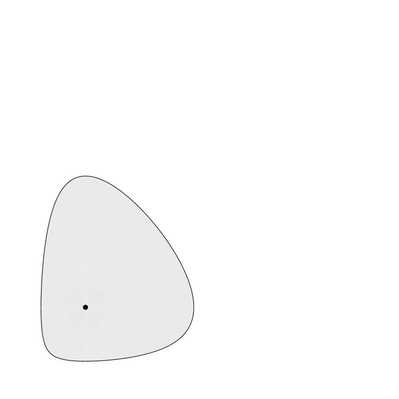
The Bregman balls of the first type are convex while this is not necessarily true for the balls of the second type as shown in Fig. 5 for the Itakura-Saito divergence (defined in Table 1). The associated bounding Bregman spheres are obtained by replacing the inequalities by equalities.
Refer to caption Refer to caption Refer to caption
(a) (b) (c)
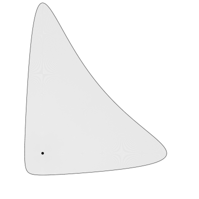
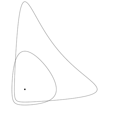
Figure 5: Bregman balls for the Itakura-Saito divergence. The (convex) ball (a) of the first type BF(𝐜,r)subscript𝐵𝐹𝐜𝑟B_{F}(\mathbf{c},r), (b) the ball of the second type BF(𝐜,r)superscriptsubscript𝐵𝐹𝐜𝑟B_{F}^{\prime}(\mathbf{c},r) with the same center and radius, (c) superposition of the two corresponding bounding spheres.

From Lemma 3, we deduce that

BF(𝐜,r)=1F(BF(𝐜,r)).superscriptsubscript𝐵𝐹𝐜𝑟superscriptbold-∇1𝐹subscript𝐵superscript𝐹superscript𝐜𝑟B_{F}^{\prime}(\mathbf{c},r)={{\bm{\nabla}^{-1}F}}(B_{F^{*}}(\mathbf{c}^{\prime},r)). (9)

Let us now examine a few properties of Bregman spheres using a lifting transformation that generalizes a similar construct for Euclidean spheres (see [10, 33]).

Let us embed the domain 𝒳𝒳\mathcal{X} in 𝒳^=𝒳×d+1^𝒳𝒳superscript𝑑1\hat{\mathcal{X}}=\mathcal{X}\times\mathbb{R}\subset\mathbb{R}^{d+1} using an extra dimension denoted by the Z𝑍Z-axis. For a point 𝐱𝒳𝐱𝒳\mathbf{x}\in\mathcal{X}, recall that 𝐱^=(𝐱,F(𝐱))^𝐱𝐱𝐹𝐱\hat{\mathbf{x}}=(\mathbf{x},F(\mathbf{x})) denotes the point obtained by lifting 𝐱𝐱\mathbf{x} onto \mathcal{F} (see Figure 1). In addition, write Proj𝒳(𝐱,z)=𝐱subscriptProj𝒳𝐱𝑧𝐱\mathrm{Proj}_{\mathcal{X}}(\mathbf{x},z)=\mathbf{x} for the projection of a point of 𝒳^^𝒳\hat{\mathcal{X}} onto 𝒳𝒳\mathcal{X}.

Let 𝐩𝒳𝐩𝒳\mathbf{p}\in\mathcal{X} and H𝐩subscript𝐻𝐩H_{\mathbf{p}} be the hyperplane tangent to \mathcal{F} at point 𝐩^^𝐩\hat{\mathbf{p}} of equation

z=H𝐩(𝐱)=𝐱𝐩,𝐩+F(𝐩),𝑧subscript𝐻𝐩𝐱𝐱𝐩superscript𝐩𝐹𝐩z=H_{\mathbf{p}}(\mathbf{x})={\langle{\mathbf{x}-\mathbf{p}},{\mathbf{p}^{\prime}}\rangle}+F(\mathbf{p}),

and let H𝐩superscriptsubscript𝐻𝐩H_{\mathbf{p}}^{\uparrow} denote the halfspace above H𝐩subscript𝐻𝐩H_{\mathbf{p}} consisting of the points 𝐱=[𝐱z]T𝒳^𝐱superscriptdelimited-[]𝐱𝑧𝑇^𝒳\mathbf{x}=[\mathbf{x}\ z]^{T}\in\hat{\mathcal{X}} such that z>H𝐩(𝐱)𝑧subscript𝐻𝐩𝐱z>H_{\mathbf{p}}(\mathbf{x}). Let σ(𝐜,r)𝜎𝐜𝑟\sigma(\mathbf{c},r) denote either the first-type or second-type Bregman sphere centered at 𝐜𝐜\mathbf{c} with radius r𝑟r (i.e., BF(𝐜,r)subscript𝐵𝐹𝐜𝑟\partial B_{F}(\mathbf{c},r) or BF(𝐜,r)superscriptsubscript𝐵𝐹𝐜𝑟\partial B_{F}^{\prime}(\mathbf{c},r)).

The lifted image σ^^𝜎\hat{\sigma} of a Bregman sphere σ𝜎\sigma is σ^={(𝐱,F(𝐱)),𝐱σ}^𝜎𝐱𝐹𝐱𝐱𝜎\hat{\sigma}=\{(\mathbf{x},F(\mathbf{x})),\mathbf{x}\in\sigma\}. We associate to a Bregman sphere σ=σ(𝐜,r)𝜎𝜎𝐜𝑟\sigma=\sigma(\mathbf{c},r) of 𝒳𝒳\mathcal{X} the hyperplane

Hσ:z=𝐱𝐜,𝐜+F(𝐜)+r,:subscript𝐻𝜎𝑧𝐱𝐜superscript𝐜𝐹𝐜𝑟H_{\sigma}:z={\langle{\mathbf{x}-\mathbf{c}},{\mathbf{c}^{\prime}}\rangle}+F(\mathbf{c})+r, (10)

parallel to H𝐜subscript𝐻𝐜H_{\mathbf{c}} and at vertical distance r𝑟r from H𝐜subscript𝐻𝐜H_{\mathbf{c}} (see Figure 6). Observe that Hσsubscript𝐻𝜎H_{\sigma} coincides with H𝐜subscript𝐻𝐜H_{\mathbf{c}} when r=0𝑟0r=0, i.e. when sphere σ𝜎\sigma is reduced to a single point.

Lemma 5

σ^^𝜎\hat{\sigma} is the intersection of \mathcal{F} with Hσsubscript𝐻𝜎H_{\sigma}. Conversely, the intersection of any hyperplane H𝐻H with \mathcal{F} projects onto 𝒳𝒳\mathcal{X} as a Bregman sphere. More precisely, if the equation of H𝐻H is z=𝐱,𝐚+b𝑧𝐱𝐚𝑏z={\langle{\mathbf{x}},{\mathbf{a}}\rangle}+b, the sphere is centered at 𝐜=1F(𝐚)𝐜superscriptbold-∇1𝐹𝐚\mathbf{c}={{\bm{\nabla}^{-1}F}}(\mathbf{a}) and its radius is 𝐚,𝐜F(𝐜)+b𝐚𝐜𝐹𝐜𝑏{\langle{\mathbf{a}},{\mathbf{c}}\rangle}-F(\mathbf{c})+b.

Proof: The first part of the lemma is a direct consequence of the fact that DF(𝐱||𝐲)D_{F}(\mathbf{x}||\mathbf{y}) is measured by the vertical distance from 𝐱^^𝐱\hat{\mathbf{x}} to H𝐲subscript𝐻𝐲H_{\mathbf{y}} (see Lemma 1). For the second part, we consider the hyperplane Hsuperscript𝐻H^{\|} parallel to H𝐻H and tangent to \mathcal{F}. From Eq. 10, we deduce 𝐚=𝐜𝐚superscript𝐜\mathbf{a}=\mathbf{c}^{\prime}. The equation of Hsuperscript𝐻H^{\|} is thus z=𝐱1F(𝐚),𝐚+F(1F(𝐚))𝑧𝐱superscriptbold-∇1𝐹𝐚𝐚𝐹superscriptbold-∇1𝐹𝐚z={\langle{\mathbf{x}-{{\bm{\nabla}^{-1}F}}(\mathbf{a})},{\mathbf{a}}\rangle}+F({{\bm{\nabla}^{-1}F}}(\mathbf{a})). It follows that the divergence from any point of σ𝜎\sigma to 𝐜𝐜\mathbf{c}, which is equal to the vertical distance between H𝐻H and Hsuperscript𝐻H^{\|}, is 1F(𝐚),𝐚F(1F(𝐚))+b=𝐚,𝐜F(𝐜)+bsuperscriptbold-∇1𝐹𝐚𝐚𝐹superscriptbold-∇1𝐹𝐚𝑏𝐚𝐜𝐹𝐜𝑏{\langle{{{\bm{\nabla}^{-1}F}}(\mathbf{a})},{\mathbf{a}}\rangle}-F({{\bm{\nabla}^{-1}F}}(\mathbf{a}))+b={\langle{\mathbf{a}},{\mathbf{c}}\rangle}-F(\mathbf{c})+b. \square

Refer to caption Refer to caption
(a) Squared Euclidean distance (b) Itakura-Saito divergence
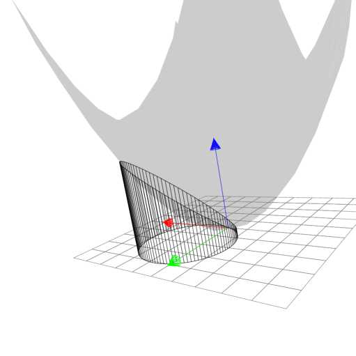
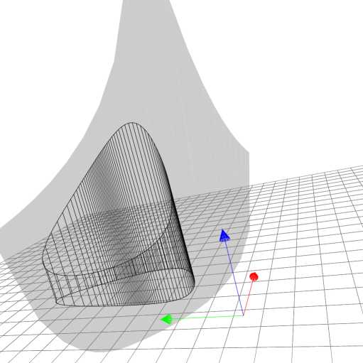
Figure 6: Two Bregman circles σ𝜎\sigma and the associated curves σ^^𝜎\hat{\sigma} obtained by lifting σ𝜎\sigma onto \mathcal{F}. The curves σ^^𝜎\hat{\sigma} are obtained as the intersection of the hyperplane Hσsubscript𝐻𝜎H_{\sigma} with the convex hypersurface \mathcal{F}. 3D illustration with (a) the squared Euclidean distance, and (b) the Itakura-Saito divergence.

Bregman spheres have been defined as manifolds of codimension 1 of dsuperscript𝑑\mathbb{R}^{d}, i.e. hyperspheres. More generally, we can define the Bregman spheres of codimension k+1𝑘1k+1 of dsuperscript𝑑\mathbb{R}^{d} as the Bregman (hyper)spheres of some affine space 𝒵d𝒵superscript𝑑\mathcal{Z}\subset\mathbb{R}^{d} of codimension k𝑘k. The next lemma shows that Bregman spheres are stable under intersection.

Lemma 6

The intersection of k𝑘k Bregman spheres σ1,,σksubscript𝜎1subscript𝜎𝑘\sigma_{1},\ldots,\sigma_{k} is a Bregman sphere σ𝜎\sigma. If the σisubscript𝜎𝑖\sigma_{i} pairwise intersect transversally, σ=i=1kσi𝜎superscriptsubscript𝑖1𝑘subscript𝜎𝑖\sigma=\cap_{i=1}^{k}\sigma_{i} is a k𝑘k-Bregman sphere.

Proof: Consider first the case of Bregman spheres of the first type. The k𝑘k hyperplanes Hσisubscript𝐻subscript𝜎𝑖H_{\sigma_{i}}, i=1,,k𝑖1𝑘i=1,\ldots,k intersect along an affine space H𝐻H of codimension k𝑘k of d+1superscript𝑑1\mathbb{R}^{d+1} that vertically projects onto G𝐺G. Let G=G×superscript𝐺𝐺G^{\updownarrow}=G\times\mathbb{R} be the vertical flat of codimension k𝑘k that contains G𝐺G (and H𝐻H) and write G=Gsubscript𝐺superscript𝐺\mathcal{F}_{G}=\mathcal{F}\cap G^{\updownarrow} and HG=HGsubscript𝐻𝐺𝐻superscript𝐺H_{G}=H\cap G^{\updownarrow}. Note that Gsubscript𝐺\mathcal{F}_{G} is the graph of the restriction of F𝐹F to G𝐺G and that HGsubscript𝐻𝐺H_{G} is a hyperplane of Gsuperscript𝐺G^{\updownarrow}. We can therefore apply Lemma 5 in Gsuperscript𝐺G^{\updownarrow}, which proves the lemma for Bregman spheres of the first type.

The case of Bregman spheres of the second type follows from the duality of Eq. 9. \square

Union and intersection of Bregman balls
Theorem 4

The union of n𝑛n Bregman balls has combinatorial complexity Θ(nd+12)Θsuperscript𝑛𝑑12\Theta(n^{\lfloor{\frac{d+1}{2}}\rfloor}) and can be computed in time Θ(nlogn+nd+12)Θ𝑛𝑛superscript𝑛𝑑12\Theta(n\log n+n^{\lfloor{\frac{d+1}{2}}\rfloor}).

Proof: To each ball, we can associate its bounding Bregman sphere σisubscript𝜎𝑖\sigma_{i} which, by Lemma 5, is the projection by Proj𝒳subscriptProj𝒳\mathrm{Proj}_{\mathcal{X}} of the intersection of \mathcal{F} with a hyperplane Hσisubscript𝐻subscript𝜎𝑖H_{\sigma_{i}}. The points of \mathcal{F} that are below Hσisubscript𝐻subscript𝜎𝑖H_{\sigma_{i}} projects onto points that are inside the Bregman ball bounded by σisubscript𝜎𝑖\sigma_{i}. Hence, the union of the balls is the projection by Proj𝒳subscriptProj𝒳\mathrm{Proj}_{\mathcal{X}} of the complement of superscript\mathcal{F}\cap\mathcal{H}^{\uparrow} where =i=1nHσisuperscriptsuperscriptsubscript𝑖1𝑛superscriptsubscript𝐻subscript𝜎𝑖\mathcal{H}^{\uparrow}=\cap_{i=1}^{n}H_{\sigma_{i}}^{\uparrow}. superscript\mathcal{H}^{\uparrow} is a convex polytope defined as the intersection of n𝑛n half-spaces. The theorem follows from McMullen’s theorem that bounds the number of faces of a polytope [31], and Chazelle’s optimal convex hull/half-space intersection algorithm [14]. The result for the balls of the second type is deduced from the result for the balls of the first type and the duality of Eq. 9. \square

Very similar arguments prove the following theorem (just replace Hσisuperscriptsubscript𝐻subscript𝜎𝑖H_{\sigma_{i}}^{\uparrow} by the complementary halfspace Hσisuperscriptsubscript𝐻subscript𝜎𝑖H_{\sigma_{i}}^{\downarrow}).

Theorem 5

The intersection of n𝑛n Bregman balls has combinatorial complexity Θ(nd+12)Θsuperscript𝑛𝑑12\Theta(n^{\lfloor{\frac{d+1}{2}}\rfloor}) and can be computed in time Θ(nlogn+nd+12)Θ𝑛𝑛superscript𝑛𝑑12\Theta(n\log n+n^{\lfloor{\frac{d+1}{2}}\rfloor}).

Circumscribing Bregman spheres.

There exists, in general, a unique Bregman sphere passing through d+1𝑑1d+1 points of dsuperscript𝑑\mathbb{R}^{d}. This is easily shown using the lifting map since, in general, there exists a unique hyperplanes of d+1superscript𝑑1\mathbb{R}^{d+1} passing through d+1𝑑1d+1 points. The claim then follows from Lemma 5.

Deciding whether a point 𝐱𝐱\mathbf{x} falls inside, on or outside a Bregman sphere σd𝜎superscript𝑑\sigma\in\mathbb{R}^{d} passing through d+1𝑑1d+1 points of 𝐩0,,𝐩dsubscript𝐩0subscript𝐩𝑑\mathbf{p}_{0},...,\mathbf{p}_{d} will be crucial for computing Bregman Voronoi diagrams and associated triangulations. The lifting map immediately implies that such a decision task reduces to determining the orientation of the simplex (𝐩^0,,𝐩^d,𝐱^)subscript^𝐩0subscript^𝐩𝑑^𝐱(\mathbf{\hat{p}}_{0},...,\mathbf{\hat{p}}_{d},\hat{\mathbf{x}}) of d+1superscript𝑑1\mathbb{R}^{d+1}, which in turn reduces to evaluating the sign of the determinant of the (d+2)×(d+2)𝑑2𝑑2(d+2)\times(d+2) matrix (see [32])

InSphere(𝐱;𝐩0,,𝐩d)=|111𝐩0𝐩d𝐱F(𝐩0)F(𝐩d)F(𝐱)|InSphere𝐱subscript𝐩0subscript𝐩𝑑111subscript𝐩0subscript𝐩𝑑𝐱𝐹subscript𝐩0𝐹subscript𝐩𝑑𝐹𝐱\texttt{InSphere}(\mathbf{x};\mathbf{p}_{0},...,\mathbf{p}_{d})=\left|\begin{array}[]{cccc}1&...&1&1\\ \mathbf{p}_{0}&...&\mathbf{p}_{d}&\mathbf{x}\\ F(\mathbf{p}_{0})&...&F(\mathbf{p}_{d})&F(\mathbf{x})\end{array}\right|

If one assumes that the determinant |11𝐩0𝐩d|11subscript𝐩0subscript𝐩𝑑\left|\begin{array}[]{ccc}1&...&1\\ \mathbf{p}_{0}&...&\mathbf{p}_{d}\end{array}\right| is non-zero, InSphere(𝐱;𝐩0,,𝐩d)InSphere𝐱subscript𝐩0subscript𝐩𝑑\texttt{InSphere}(\mathbf{x};\mathbf{p}_{0},...,\mathbf{p}_{d}) is negative, null or positive depending on whether 𝐱𝐱\mathbf{x} lies inside, on, or outside σ𝜎\sigma.

3.3 Projection, orthogonality and geodesics

We start with an easy property of Bregman divergences.

Property 5 (Three-point property)

For any triple 𝐩,𝐪𝐩𝐪\mathbf{p},\mathbf{q} and 𝐫𝐫\mathbf{r} of points of 𝒳𝒳\mathcal{X}, we have:
DF(𝐩||𝐪)+DF(𝐪||𝐫)=DF(𝐩||𝐫)+𝐩𝐪,𝐫𝐪D_{F}(\mathbf{p}||\mathbf{q})+D_{F}(\mathbf{q}||\mathbf{r})=D_{F}(\mathbf{p}||\mathbf{r})+{\langle{\mathbf{p}-\mathbf{q}},{\mathbf{r}^{\prime}-\mathbf{q}^{\prime}}\rangle}.

The following lemma characterizes the Bregman projection of a point onto a closed convex set 𝒲𝒲\mathcal{W}.

Lemma 7 (Bregman projection)

For any 𝐩𝐩\mathbf{p}, there exists a unique point 𝐱𝒲𝐱𝒲\mathbf{x}\in\mathcal{W} that minimizes DF(𝐱||𝐩)D_{F}(\mathbf{x}||\mathbf{p}). We call this point the Bregman projection of 𝐩𝐩\mathbf{p} onto 𝒲𝒲\mathcal{W} and denote it 𝐩𝒲subscript𝐩𝒲\mathbf{p}_{\mathcal{W}}.

Proof: If it is not the case, then define 𝐱𝐱\mathbf{x} and 𝐲𝐲\mathbf{y} two minimizers with DF(𝐱||𝐩)=DF(𝐲||𝐩)=lD_{F}(\mathbf{x}||\mathbf{p})=D_{F}(\mathbf{y}||\mathbf{p})=l. Since 𝒲𝒲\mathcal{W} is convex, (𝐱+𝐲)/2𝒲𝐱𝐲2𝒲(\mathbf{x}+\mathbf{y})/2\in{\mathcal{W}} and, since DFsubscript𝐷𝐹D_{F} is strictly convex in its first argument (see Section 2.1), DF((𝐱+𝐲)/2||𝐩)<DF(𝐱||𝐩)/2+DF(𝐲||𝐩)/2D_{F}((\mathbf{x}+\mathbf{y})/2||\mathbf{p})<D_{F}(\mathbf{x}||\mathbf{p})/2+D_{F}(\mathbf{y}||\mathbf{p})/2. But DF(𝐱||𝐩)/2+DF(𝐲||𝐩)/2=lD_{F}(\mathbf{x}||\mathbf{p})/2+D_{F}(\mathbf{y}||\mathbf{p})/2=l yielding a contradiction. \square

We now introduce the notion of Bregman orthogonality. We say that 𝐩𝐪𝐩𝐪\mathbf{p}\mathbf{q} is Bregman orthogonal to 𝐪𝐫𝐪𝐫\mathbf{q}\mathbf{r} iff DF(𝐩||𝐪)+DF(𝐪||𝐫)=DF(𝐩||𝐫)D_{F}(\mathbf{p}||\mathbf{q})+D_{F}(\mathbf{q}||\mathbf{r})=D_{F}(\mathbf{p}||\mathbf{r}) or equivalently (by the Three-point property), if and only if 𝐩𝐪,𝐫𝐪=0𝐩𝐪superscript𝐫superscript𝐪0{\langle{\mathbf{p}-\mathbf{q}},{\mathbf{r}^{\prime}-\mathbf{q}^{\prime}}\rangle}=0. Observe the analogy with Pythagoras’ theorem in Euclidean space (see Figure 7). Note also that the orthogonality relation is not symmetric: the fact that 𝐩𝐪𝐩𝐪\mathbf{p}\mathbf{q} is Bregman orthogonal to 𝐪𝐫𝐪𝐫\mathbf{q}\mathbf{r} does not necessarily imply that 𝐪𝐫𝐪𝐫\mathbf{q}\mathbf{r} is Bregman orthogonal to 𝐩𝐪𝐩𝐪\mathbf{p}\mathbf{q}. More generally, we say that I𝒳𝐼𝒳I\subseteq{\mathcal{X}} is Bregman orthogonal to J𝒳𝐽𝒳J\subseteq{\mathcal{X}} (IJ𝐼𝐽I\cap J\neq\emptyset) iff for any 𝐩I𝐩𝐼\mathbf{p}\in I and 𝐫J𝐫𝐽\mathbf{r}\in J, there exists a 𝐪IJ𝐪𝐼𝐽\mathbf{q}\in I\cap J such that 𝐩𝐪𝐩𝐪\mathbf{p}\mathbf{q} is Bregman orthogonal to 𝐪𝐫𝐪𝐫\mathbf{q}\mathbf{r}.

Notice that orthogonality is preserved in the gradient space. Indeed, since 𝐩𝐪,𝐫𝐪=𝐫𝐪,𝐩𝐪𝐩𝐪superscript𝐫superscript𝐪superscript𝐫superscript𝐪𝐩𝐪{\langle{\mathbf{p}-\mathbf{q}},{\mathbf{r}^{\prime}-\mathbf{q}^{\prime}}\rangle}={\langle{\mathbf{r}^{\prime}-\mathbf{q}^{\prime}},{\mathbf{p}-\mathbf{q}}\rangle}, 𝐩𝐪𝐩𝐪\mathbf{p}\mathbf{q} is Bregman orthogonal to 𝐪𝐫𝐪𝐫\mathbf{q}\mathbf{r} iff 𝐫𝐪superscript𝐫superscript𝐪\mathbf{r}^{\prime}\mathbf{q}^{\prime} is Bregman orthogonal to 𝐪𝐩superscript𝐪superscript𝐩\mathbf{q}^{\prime}\mathbf{p^{\prime}}.

Refer to caption
Figure 7: Generalized Pythagoras’ theorem for Bregman divergences: The projection 𝐩𝒲subscript𝐩𝒲\mathbf{p}_{\mathcal{W}} of point 𝐩𝐩\mathbf{p} to a convex subset 𝒲𝒳𝒲𝒳\mathcal{W}\subseteq\mathcal{X}. For convex subset 𝒲𝒲\mathcal{W}, we have DF(𝐰||𝐩)DF(𝐰||𝐩𝒲)+DF(𝐩𝒲||𝐩)D_{F}(\mathbf{w}||\mathbf{p})\geq D_{F}(\mathbf{w}||\mathbf{p}_{\mathcal{W}})+D_{F}(\mathbf{p}_{\mathcal{W}}||\mathbf{p}) (with equality for and only for affine sets 𝒲𝒲\mathcal{W}).

Let ΓF(𝐩,𝐪)subscriptΓ𝐹𝐩𝐪\Gamma_{F}(\mathbf{p},\mathbf{q}) be the image by 1Fsuperscriptbold-∇1𝐹{{\bm{\nabla}^{-1}F}} of the line segment 𝐩𝐪superscript𝐩superscript𝐪\mathbf{p}^{\prime}\mathbf{q}^{\prime}, i.e.

ΓF(𝐩,𝐪)={𝐱𝒳:𝐱=(1λ)𝐩+λ𝐪,λ[0,1]}.subscriptΓ𝐹𝐩𝐪conditional-set𝐱𝒳formulae-sequencesuperscript𝐱1𝜆superscript𝐩𝜆superscript𝐪𝜆01\Gamma_{F}(\mathbf{p},\mathbf{q})=\{\mathbf{x}\in\mathcal{X}:\mathbf{x}^{\prime}=(1-\lambda)\mathbf{p}^{\prime}+\lambda\mathbf{q}^{\prime},\lambda\in[0,1]\}.

By analogy, we rename the line segment 𝐩𝐪𝐩𝐪\mathbf{p}\mathbf{q} as

Λ(𝐩,𝐪)={𝐱𝒳:𝐱=(1λ)𝐩+λ𝐪,λ[0,1]}Λ𝐩𝐪conditional-set𝐱𝒳formulae-sequence𝐱1𝜆𝐩𝜆𝐪𝜆01\Lambda(\mathbf{p},\mathbf{q})=\{\mathbf{x}\in{\mathcal{X}}:\mathbf{x}=(1-\lambda)\mathbf{p}+\lambda\mathbf{q},\lambda\in[0,1]\}

In the Euclidean case (F(x)=12𝐱2𝐹𝑥12superscriptnorm𝐱2F(x)=\frac{1}{2}\|\mathbf{x}\|^{2}), ΓF(𝐩,𝐪)=Λ(𝐩,𝐪)subscriptΓ𝐹𝐩𝐪Λ𝐩𝐪\Gamma_{F}(\mathbf{p},\mathbf{q})=\Lambda(\mathbf{p},\mathbf{q}) is the unique geodesic path joining 𝐩𝐩\mathbf{p} to 𝐪𝐪\mathbf{q} and it is orthogonal to the bisector HF(𝐩,𝐪)subscript𝐻𝐹𝐩𝐪H_{F}(\mathbf{p},\mathbf{q}). For general Bregman divergences, we have similar properties as shown next.

Lemma 8

ΓF(𝐩,𝐪)subscriptΓ𝐹𝐩𝐪\Gamma_{F}(\mathbf{p},\mathbf{q}) is Bregman orthogonal to the Bregman bisector HF(𝐩,𝐪)subscript𝐻𝐹𝐩𝐪H_{F}(\mathbf{p},\mathbf{q}) while Λ(𝐩,𝐪)Λ𝐩𝐪\Lambda(\mathbf{p},\mathbf{q}) is Bregman orthogonal to HF(𝐩,𝐪)subscript𝐻superscript𝐹𝐩𝐪H_{F^{*}}(\mathbf{p},\mathbf{q}).

Proof: Since 𝐩𝐩\mathbf{p} and 𝐪𝐪\mathbf{q} lie on different sides of HF(𝐩,𝐪)subscript𝐻𝐹𝐩𝐪H_{F}(\mathbf{p},\mathbf{q}), ΓF(𝐩,𝐪)subscriptΓ𝐹𝐩𝐪\Gamma_{F}(\mathbf{p},\mathbf{q}) must intersect HF(𝐩,𝐪)subscript𝐻𝐹𝐩𝐪H_{F}(\mathbf{p},\mathbf{q}). Fix any distinct 𝐱Γ(𝐩,𝐪)𝐱Γ𝐩𝐪\mathbf{x}\in\Gamma(\mathbf{p},\mathbf{q}) and 𝐲HF(𝐩,𝐪)𝐲subscript𝐻𝐹𝐩𝐪\mathbf{y}\in H_{F}(\mathbf{p},\mathbf{q}), and let 𝐭Γ(𝐩,𝐪)HF(𝐩,𝐪)𝐭Γ𝐩𝐪subscript𝐻𝐹𝐩𝐪\mathbf{t}\in\Gamma(\mathbf{p},\mathbf{q})\cap H_{F}(\mathbf{p},\mathbf{q}). To prove the first part of the lemma, we need to show that 𝐲𝐭,𝐱𝐭=0𝐲𝐭superscript𝐱superscript𝐭0{\langle{\mathbf{y}-\mathbf{t}},{\mathbf{x}^{\prime}-\mathbf{t}^{\prime}}\rangle}=0.

Since 𝐭𝐭\mathbf{t} and 𝐱𝐱\mathbf{x} both belong to ΓF(𝐩,𝐪)absentsubscriptΓ𝐹𝐩𝐪\in\Gamma_{F}(\mathbf{p},\mathbf{q}), we have 𝐭𝐱=λ(𝐩𝐪)superscript𝐭superscript𝐱𝜆superscript𝐩superscript𝐪\mathbf{t}^{\prime}-\mathbf{x}^{\prime}=\lambda(\mathbf{p}^{\prime}-\mathbf{q}^{\prime}), for some λ𝜆\lambda\in\mathbb{R}, and, since 𝐲𝐲\mathbf{y} and 𝐭𝐭\mathbf{t} belong to HF(𝐩,𝐪)subscript𝐻𝐹𝐩𝐪H_{F}(\mathbf{p},\mathbf{q}), we deduce from the equation of HF(𝐩,𝐪)subscript𝐻𝐹𝐩𝐪H_{F}(\mathbf{p},\mathbf{q}) that 𝐲𝐭,𝐩𝐪=0𝐲𝐭superscript𝐩superscript𝐪0{\langle{\mathbf{y}-\mathbf{t}},{\mathbf{p}^{\prime}-\mathbf{q}^{\prime}}\rangle}=0. We conclude that 𝐲𝐭,𝐱𝐭=0𝐲𝐭superscript𝐱superscript𝐭0{\langle{\mathbf{y}-\mathbf{t}},{\mathbf{x}^{\prime}-\mathbf{t}^{\prime}}\rangle}=0, which proves that ΓF(𝐩,𝐪)subscriptΓ𝐹𝐩𝐪\Gamma_{F}(\mathbf{p},\mathbf{q}) is indeed Bregman orthogonal to HF(𝐩,𝐪)subscript𝐻𝐹𝐩𝐪H_{F}(\mathbf{p},\mathbf{q}).

The second part of the lemma is easily proved by using the fact that orthogonality is preserved in the gradient space as noted above. \square
Refer to caption
Refer to caption
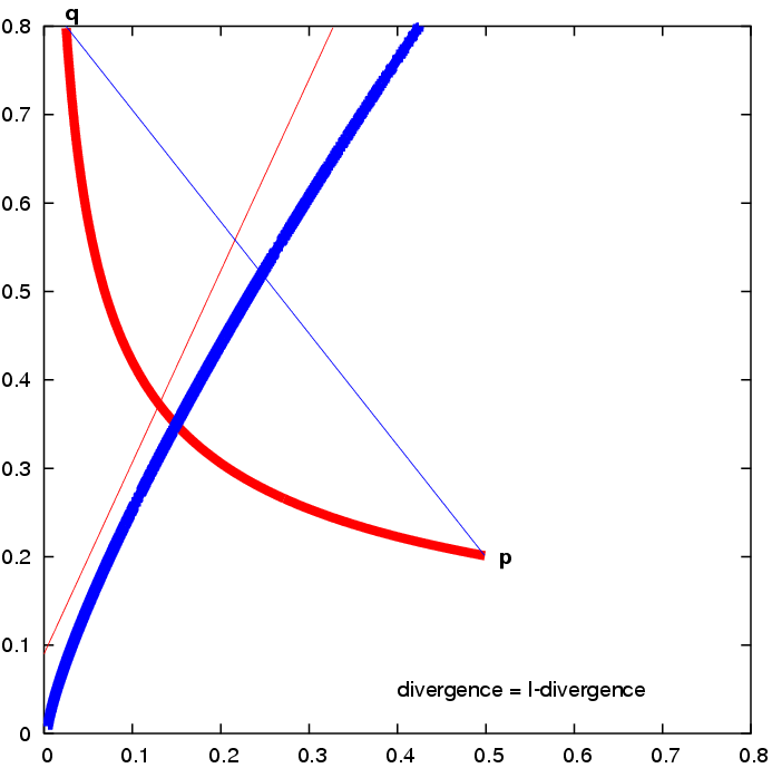
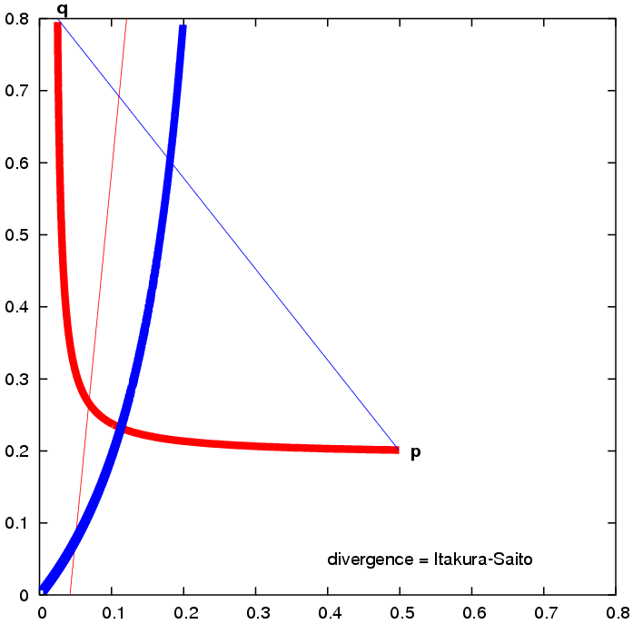
Figure 8: Bregman bisectors and their relationships with respect to Λ(𝐩,𝐪)Λ𝐩𝐪\Lambda(\mathbf{p},\mathbf{q}) (straight line segments) and ΓF(𝐩,𝐪)subscriptΓ𝐹𝐩𝐪\Gamma_{F}(\mathbf{p},\mathbf{q}) (bold curves), for the Itakura-Saito divergence (left) and I-divergence (right). Bold curves become linear in 𝒳superscript𝒳\mathcal{X}^{\prime}; colors depict the Bregman orthogonality relationships of Lemma 8.

Figure 8 shows Bregman bisectors and their relationships with respect to Λ(𝐩,𝐪)Λ𝐩𝐪\Lambda(\mathbf{p},\mathbf{q}) and ΓF(𝐩,𝐪)subscriptΓ𝐹𝐩𝐪\Gamma_{F}(\mathbf{p},\mathbf{q}).

We now focus on characterizing Bregman geodesics. First, recall that a parameterized curve 𝒞𝒞{\mathcal{C}} between two points 𝐩0subscript𝐩0\mathbf{p}_{0} and 𝐩1subscript𝐩1\mathbf{p}_{1} is defined as a set 𝒞={𝐩λ}λ=01𝒞superscriptsubscriptsubscript𝐩𝜆𝜆01{\mathcal{C}}=\{\mathbf{p}_{\lambda}\}_{\lambda=0}^{1}, which is continuous. In Riemannian geometry, geodesics are the curves that minimize the arc length with respect to the Riemannian metric [1, 27]. Since embedding 𝒳𝒳\mathcal{X} with a Bregman divergence does not yield a metric space, we define the following curve lengths:

Γ(𝒞)subscriptΓ𝒞\displaystyle\ell_{\Gamma}({\mathcal{C}}) =\displaystyle= λ=01DF(𝒑0||𝒑λ)dλ,\displaystyle\int_{\lambda=0}^{1}{D_{F}(\bm{p}_{0}||\bm{p}_{\lambda})\mathrm{d}\lambda}\>\>, (11)
Λ(𝒞)subscriptΛ𝒞\displaystyle\ell_{\Lambda}({\mathcal{C}}) =\displaystyle= λ=01DF(𝒑λ||𝒑0)dλ.\displaystyle\int_{\lambda=0}^{1}{D_{F}(\bm{p}_{\lambda}||\bm{p}_{0})\mathrm{d}\lambda}. (12)

We now characterize the dual pair of geodesics and their lengths as follows:

Lemma 9

Curve ΓF(𝐩0,𝐩1)subscriptΓ𝐹subscript𝐩0subscript𝐩1\Gamma_{F}(\mathbf{p}_{0},\mathbf{p}_{1}) (respectively straight line segment Λ(𝐩0,𝐩1)Λsubscript𝐩0subscript𝐩1\Lambda(\mathbf{p}_{0},\mathbf{p}_{1})) minimizes λ=01DF(𝐩0||𝐩λ)dλ\int_{\lambda=0}^{1}{D_{F}(\mathbf{p}_{0}||\mathbf{p}_{\lambda})\mathrm{d}\lambda} (respectively λ=01DF(𝐩λ||𝐩0)dλ\int_{\lambda=0}^{1}{D_{F}(\bm{p}_{\lambda}||\bm{p}_{0})\mathrm{d}\lambda}) over all curves 𝒞={𝐩λ}λ=01𝒞superscriptsubscriptsubscript𝐩𝜆𝜆01\mathcal{C}=\{\mathbf{p}_{\lambda}\}_{\lambda=0}^{1}.

Proof: For any curve 𝒞𝒞{\mathcal{C}} between 𝐩0subscript𝐩0\mathbf{p}_{0} and 𝐩1subscript𝐩1\mathbf{p}_{1}, we measure the ΓsubscriptΓ\ell_{\Gamma} length as Γ(𝒞)=λDF(𝐩λ||𝐩0)dλ\ell_{\Gamma}({\mathcal{C}})=\int_{\lambda}{D_{F}(\mathbf{p}_{\lambda}||\mathbf{p}_{0})\mathrm{d}\lambda}. Fix some inner point 𝐩ΓF(𝐩0,𝐩1)\{𝐩0,𝐩1}𝐩\subscriptΓ𝐹subscript𝐩0subscript𝐩1subscript𝐩0subscript𝐩1\mathbf{p}\in\Gamma_{F}(\mathbf{p}_{0},\mathbf{p}_{1})\backslash\{\mathbf{p}_{0},\mathbf{p}_{1}\}. From the three-point property (Property 5), the set of points {𝐲𝒳|DF(𝐲||𝐩0)=DF(𝐲||𝐩)+DF(𝐩||𝐩0)}\{\mathbf{y}\in\mathcal{X}\ |\ D_{F}(\mathbf{y}||\mathbf{p}_{0})=D_{F}(\mathbf{y}||\mathbf{p})+D_{F}(\mathbf{p}||\mathbf{p}_{0})\} is the hyperplane H𝐩:𝐲,𝐡=b:subscript𝐻𝐩𝐲𝐡𝑏H_{\mathbf{p}}:{\langle{\mathbf{y}},{\mathbf{h}}\rangle}=b (𝐡𝐡\mathbf{h} is a perpendicular vector to the hyperplane) which splits 𝒳𝒳\mathcal{X} into two open half-spaces H𝐩+:𝐲,𝐡>b:superscriptsubscript𝐻𝐩𝐲𝐡𝑏H_{\mathbf{p}}^{+}:{\langle{\mathbf{y}},{\mathbf{h}}\rangle}>b, and H𝐩:𝐲,𝐡<b:superscriptsubscript𝐻𝐩𝐲𝐡𝑏H_{\mathbf{p}}^{-}:{\langle{\mathbf{y}},{\mathbf{h}}\rangle}<b. Now, H𝐩subscript𝐻𝐩H_{\mathbf{p}} intersects Γ(𝐩0,𝐩1)Γsubscript𝐩0subscript𝐩1\Gamma(\mathbf{p}_{0},\mathbf{p}_{1}) since H𝐩subscript𝐻𝐩H_{\mathbf{p}} separates 𝐩0subscript𝐩0\mathbf{p}_{0} from 𝐩1subscript𝐩1\mathbf{p}_{1}. Indeed, H𝐩(𝐩0)=𝐩0𝐩,𝐩0𝐩=DF(𝐩0||𝐩)+DF(𝐩||𝐩0)>0H_{\mathbf{p}}(\mathbf{p}_{0})={\langle{\mathbf{p}_{0}-\mathbf{p}},{\mathbf{p}_{0}^{\prime}-\mathbf{p}^{\prime}}\rangle}=D_{F}(\mathbf{p}_{0}||\mathbf{p})+D_{F}(\mathbf{p}||\mathbf{p}_{0})>0 and H𝐩(𝐩1)=𝐩1𝐩,𝐩0𝐩=λ1λ𝐩1𝐩,𝐩1𝐩<0subscript𝐻𝐩subscript𝐩1subscript𝐩1𝐩superscriptsubscript𝐩0superscript𝐩𝜆1𝜆subscript𝐩1𝐩superscriptsubscript𝐩1superscript𝐩0H_{\mathbf{p}}(\mathbf{p}_{1})={\langle{\mathbf{p}_{1}-\mathbf{p}},{\mathbf{p}_{0}^{\prime}-\mathbf{p}^{\prime}}\rangle}=\frac{\lambda-1}{\lambda}{\langle{\mathbf{p}_{1}-\mathbf{p}},{\mathbf{p}_{1}^{\prime}-\mathbf{p}^{\prime}}\rangle}<0 where 𝐩=λ𝐩0+(1λ)𝐩1superscript𝐩𝜆superscriptsubscript𝐩01𝜆superscriptsubscript𝐩1\mathbf{p}^{\prime}=\lambda\mathbf{p}_{0}^{\prime}+(1-\lambda)\mathbf{p}_{1}^{\prime} (with λ]0,1[\lambda\in]0,1[). Therefore any connected path 𝒞𝒞\mathcal{C} joining 𝐩0subscript𝐩0\mathbf{p}_{0} to 𝐩1subscript𝐩1\mathbf{p}_{1} has to intersect H𝐩subscript𝐻𝐩H_{\mathbf{p}}.

To finish up, consider function f:[0,1]𝒞:𝑓01𝒞f:[0,1]\rightarrow{\mathcal{C}} with f(0)=𝐩0𝑓0subscript𝐩0f(0)=\mathbf{p}_{0}, f(1)=𝐩1𝑓1subscript𝐩1f(1)=\mathbf{p}_{1}, and f(λ)𝒞H𝐩λ𝑓𝜆𝒞subscript𝐻subscript𝐩𝜆f(\lambda)\in{\mathcal{C}}\cap H_{\mathbf{p}_{\lambda}} otherwise, where it is understood that 𝐩λsubscript𝐩𝜆\mathbf{p}_{\lambda} is hereafter a point of ΓF(𝐩0,𝐩1)subscriptΓ𝐹subscript𝐩0subscript𝐩1\Gamma_{F}(\mathbf{p}_{0},\mathbf{p}_{1}). Since f(λ)H𝐩(λ)𝑓𝜆subscript𝐻𝐩𝜆f(\lambda)\in H_{\mathbf{p}(\lambda)}, we have DF(f(λ)||𝐩0)=DF(f(λ)||𝐩λ)+DF(𝐩λ||𝐩0)DF(𝐩λ||𝐩0)D_{F}(f(\lambda)||\mathbf{p}_{0})=D_{F}(f(\lambda)||\mathbf{p}_{\lambda})+D_{F}(\mathbf{p}_{\lambda}||\mathbf{p}_{0})\geq D_{F}(\mathbf{p}_{\lambda}||\mathbf{p}_{0}), with equality if and only if f(λ)=𝐩λ𝑓𝜆subscript𝐩𝜆f(\lambda)=\mathbf{p}_{\lambda}. Thus we have

Γ(ΓF(𝐩0,𝐩1))=λ=01DF(𝐩λ||𝐩0)dλ\displaystyle\ell_{\Gamma}(\Gamma_{F}(\mathbf{p}_{0},\mathbf{p}_{1}))=\int_{\lambda=0}^{1}{D_{F}(\mathbf{p}_{\lambda}||\mathbf{p}_{0})\mathrm{d}\lambda} \displaystyle\leq λ=01DF(f(λ)||𝐩0)dλΓ(𝒞).\displaystyle\int_{\lambda=0}^{1}{D_{F}(f(\lambda)||\mathbf{p}_{0})\mathrm{d}\lambda}\leq\ell_{\Gamma}({\mathcal{C}})\>\>.

The case of Λ(𝐩0,𝐩1)Λsubscript𝐩0subscript𝐩1\Lambda(\mathbf{p}_{0},\mathbf{p}_{1}) follows similarly from Legendre convex duality.

\square

Corollary 1

Since ΓF(𝐩0,𝐩1)=ΓF(𝐩1,𝐩0)subscriptΓ𝐹subscript𝐩0subscript𝐩1subscriptΓ𝐹subscript𝐩1subscript𝐩0\Gamma_{F}(\mathbf{p}_{0},\mathbf{p}_{1})=\Gamma_{F}(\mathbf{p}_{1},\mathbf{p}_{0}) (respectively, since Λ(𝐩0,𝐩1)=Λ(𝐩1,𝐩0)Λsubscript𝐩0subscript𝐩1Λsubscript𝐩1subscript𝐩0\Lambda(\mathbf{p}_{0},\mathbf{p}_{1})=\Lambda(\mathbf{p}_{1},\mathbf{p}_{0})) we deduce that ΓF(𝐩0,𝐩1)subscriptΓ𝐹subscript𝐩0subscript𝐩1\Gamma_{F}(\mathbf{p}_{0},\mathbf{p}_{1}) minimizes also λ=01DF(𝐩1||𝐩λ)dλ\int_{\lambda=0}^{1}{D_{F}(\mathbf{p}_{1}||\mathbf{p}_{\lambda})\mathrm{d}\lambda} (respectively, minimizes also λ=01DF(𝐩λ||𝐩1)dλ\int_{\lambda=0}^{1}{D_{F}(\mathbf{p}_{\lambda}||\mathbf{p}_{1})\mathrm{d}\lambda}) over all curves 𝒞={𝐩λ}λ=01𝒞superscriptsubscriptsubscript𝐩𝜆𝜆01\mathcal{C}=\{\mathbf{p}_{\lambda}\}_{\lambda=0}^{1}.

Observe also that ΓF(𝐩,𝐪)subscriptΓ𝐹𝐩𝐪\Gamma_{F}(\mathbf{p},\mathbf{q}) is the unique geodesic path joining 𝐩𝐩\mathbf{p} to 𝐪𝐪\mathbf{q} in 𝒳𝒳\mathcal{X} for the metric image by 1Fsuperscriptbold-∇1𝐹{{\bm{\nabla}^{-1}F}} of the Euclidean metric.

Finally, we give a characterization of these geodesics in information-theoretic spaces. Recall that Banerjee et al. [6] showed that Bregman divergences are in bijection with exponential families. This was emphasized by Theorem 2 that proved that the Kullback-Leibler divergence of probability density functions of the same exponential family Fsubscript𝐹\mathcal{E}_{F} is a Bregman divergence DFsubscript𝐷𝐹D_{F} for the cumulant function F𝐹F. From this standpoint, Λ(𝐩,𝐪)Λ𝐩𝐪\Lambda(\mathbf{p},\mathbf{q}) and ΓF(𝐩,𝐪)subscriptΓ𝐹𝐩𝐪\Gamma_{F}(\mathbf{p},\mathbf{q}) minimize the total Kullback-Leibler divergence, a characteristic that we choose to call the information length of a curve. Since the Kullback-Leibler divergence is not symmetric, this justifies for the existence of two geodesics, one which appears to be linear when parameterized with the natural affine coordinate system (𝜽𝜽{\bm{\theta}}), and the other that is linear in the expectation affine coordinate system (𝝁𝝁{\bm{\mu}}). See also [1].

Corollary 2

Suppose p(.|𝛉0)p(.|\bm{\theta}_{0}) and p(.|𝛉1)p(.|\bm{\theta}_{1}) are probability density functions of the same exponential family Fsubscript𝐹{\mathcal{E}}_{F}. Then ΓF(𝛉0,𝛉1)subscriptΓ𝐹subscript𝛉0subscript𝛉1\Gamma_{F}(\bm{\theta}_{0},\bm{\theta}_{1}) (resp. Λ(𝛉0,𝛉1)Λsubscript𝛉0subscript𝛉1\Lambda(\bm{\theta}_{0},\bm{\theta}_{1})) minimizes Γ(𝒞)=λ=01KL(𝛉0||𝛉λ)dλ\ell_{\Gamma}({\mathcal{C}})=\int_{\lambda=0}^{1}\mathrm{KL}({\bm{\theta}}_{0}||{\bm{\theta}}_{\lambda})\mathrm{d}\lambda (resp. Λ(𝒞)=λ=01KL(𝛉λ||𝛉0)dλ\ell_{\Lambda}({\mathcal{C}})=\int_{\lambda=0}^{1}\mathrm{KL}({\bm{\theta}}_{\lambda}||{\bm{\theta}}_{0})\mathrm{d}\lambda) over all curves 𝒞={p(.|𝛉λ)}λ=01\mathcal{C}=\{p(.|\bm{\theta}_{\lambda})\}_{\lambda=0}^{1}.

4 Bregman Voronoi diagrams

Let 𝒮={𝐩1,,𝐩n}𝒮subscript𝐩1subscript𝐩𝑛\mathcal{S}=\{\mathbf{p}_{1},...,\mathbf{p}_{n}\} be a finite point set of 𝒳d𝒳superscript𝑑\mathcal{X}\subset\mathbb{R}^{d}. To each point 𝐩isubscript𝐩𝑖\mathbf{p}_{i} is attached a d𝑑d-variate continuous function Disubscript𝐷𝑖D_{i} defined over 𝒳𝒳\mathcal{X}. We define the lower envelope of the functions as the graph of min1inDisubscript1𝑖𝑛subscript𝐷𝑖\min_{1\leq i\leq n}D_{i} and their minimization diagram as the subdivision of 𝒳𝒳\mathcal{X} into cells such that, in each cell, argminifisubscript𝑖subscript𝑓𝑖\arg\min_{i}f_{i} is fixed.

The Euclidean Voronoi diagram is the minimization diagram for Di(𝐱)=𝐱𝐩i2subscript𝐷𝑖𝐱superscriptnorm𝐱subscript𝐩𝑖2D_{i}(\mathbf{x})=\|\mathbf{x}-\mathbf{p}_{i}\|^{2}. In this section, we introduce Bregman Voronoi diagrams as minimization diagrams of Bregman divergences (see Figure 10).

We define three types of Bregman Voronoi diagrams in §4.1. We establish a correspondence between Bregman Voronoi diagrams and polytopes in §4.2 and with power diagrams in §4.3. These correspondences lead to tight combinatorial bounds and efficient algorithms. Finally, in §4.4, we give two generalizations of Bregman Voronoi diagrams; k𝑘k-order and k𝑘k-bag diagrams.

We note 𝒮={F(𝐩i),i=1,,n}\mathcal{S}^{\prime}=\{\bm{\nabla}_{F}(\mathbf{p}_{i}),i=1,\ldots,n\} the gradient point set associated to 𝒮𝒮\mathcal{S}.

4.1 Three types of diagrams

Because Bregman divergences are not necessarily symmetric, we associate to each site 𝐩isubscript𝐩𝑖\mathbf{p}_{i} two types of distance functions, namely Di(𝐱)=DF(𝐱||𝐩i)D_{i}(\mathbf{x})=D_{F}(\mathbf{x}||\mathbf{p}_{i}) and Di(𝐱)=DF(𝐩i||𝐱)D_{i}^{\prime}(\mathbf{x})=D_{F}(\mathbf{p}_{i}||\mathbf{x}). The minimization diagram of the Disubscript𝐷𝑖D_{i}, i=1,,n𝑖1𝑛i=1,\ldots,n, is called the first-type Bregman Voronoi diagram of 𝒮𝒮\mathcal{S}, which we denote by vorF(𝒮)subscriptvor𝐹𝒮\mathrm{vor}_{F}(\mathcal{S}). The d𝑑d-dimensional cells of this diagram are in 1-1 correspondence with the sites 𝐩isubscript𝐩𝑖\mathbf{p}_{i} and the d𝑑d-dimensional cell of 𝐩isubscript𝐩𝑖\mathbf{p}_{i} is defined as

vorF(𝐩i)=def{𝐱𝒳|DF(𝐱||𝐩i)DF(𝐱||𝐩j)𝐩j𝒮.}\mathrm{vor}_{F}(\mathbf{p}_{i})\stackrel{{\scriptstyle\mathrm{def}}}{{=}}\{\mathbf{x}\in\mathcal{X}\ |\ D_{F}(\mathbf{x}||\mathbf{p}_{i})\leq D_{F}(\mathbf{x}||\mathbf{p}_{j})\ \forall\mathbf{p}_{j}\in\mathcal{S}.\}

Since the Bregman bisectors of the first-type are hyperplanes, the cells of any diagram of the first-type are convex polyhedra. Therefore, first-type Bregman Voronoi diagrams are affine diagrams [4, 5].

Similarly, the minimization diagram of the Disuperscriptsubscript𝐷𝑖D_{i}^{\prime}, i=1,,n𝑖1𝑛i=1,\ldots,n, is called the second-type Bregman Voronoi diagram of 𝒮𝒮\mathcal{S}, which we denote by vorF(𝒮)subscriptsuperscriptvor𝐹𝒮\mathrm{vor}^{\prime}_{F}(\mathcal{S}). A cell in vorF(𝒮)subscriptsuperscriptvor𝐹𝒮\mathrm{vor}^{\prime}_{F}(\mathcal{S}) is associated to each site 𝐩isubscript𝐩𝑖\mathbf{p}_{i} and is defined as above with permuted divergence arguments:

vorF(𝐩i)=def{𝐱𝒳|DF(𝐩i||𝐱)DF(𝐩j||𝐱)𝐩j𝒮.}\mathrm{vor}^{\prime}_{F}(\mathbf{p}_{i})\stackrel{{\scriptstyle\mathrm{def}}}{{=}}\{\mathbf{x}\in\mathcal{X}\ |\ D_{F}(\mathbf{p}_{i}||\mathbf{x})\leq D_{F}(\mathbf{p}_{j}||\mathbf{x})\ \forall\mathbf{p}_{j}\in\mathcal{S}.\}

In contrast with the diagrams of the first-type, the diagrams of the second type have, in general, curved faces.

Figure 9 illustrates these Bregman Voronoi diagrams for the Kullback-Leibler and the Itakura-Saito divergences. Note that the Euclidean Voronoi diagram is a Bregman Voronoi diagram since vor(𝒮)=vorF(𝒮)=vorF(𝒮)vor𝒮subscriptvor𝐹𝒮subscriptsuperscriptvor𝐹𝒮\mathrm{vor}(\mathcal{S})=\mathrm{vor}_{F}(\mathcal{S})=\mathrm{vor}^{\prime}_{F}(\mathcal{S}) for F(𝐱)=𝐱2𝐹𝐱superscriptnorm𝐱2F(\mathbf{x})=\|\mathbf{x}\|^{2}.

For asymmetric Bregman divergences DFsubscript𝐷𝐹D_{F}, we can further consider the symmetrized Bregman divergence SF=DF~subscript𝑆𝐹subscript𝐷~𝐹S_{F}=D_{\tilde{F}} and define a third-type Bregman Voronoi diagram vorF′′(𝒮)subscriptsuperscriptvor′′𝐹𝒮\mathrm{vor}^{\prime\prime}_{F}(\mathcal{S}). The cell of vorF′′(𝒮)subscriptsuperscriptvor′′𝐹𝒮\mathrm{vor}^{\prime\prime}_{F}(\mathcal{S}) associated to site 𝐩isubscript𝐩𝑖\mathbf{p}_{i} is defined as:

vorF′′(𝐩i)=def{𝐱𝒳|SF(𝐱,𝐩i)SF(𝐱,𝐩j)𝐩j𝒮.}\mathrm{vor}^{\prime\prime}_{F}(\mathbf{p}_{i})\stackrel{{\scriptstyle\mathrm{def}}}{{=}}\{\mathbf{x}\in\mathcal{X}\ |\ S_{F}(\mathbf{x},\mathbf{p}_{i})\leq S_{F}(\mathbf{x},\mathbf{p}_{j})\ \forall\mathbf{p}_{j}\in\mathcal{S}.\}
Refer to caption Refer to caption
(a) (b)
Figure 9: Three types of Bregman Voronoi diagrams for (a) the Kullback-Leibler and (b) the Itakura-Saito divergences. First-type affine Bregman Voronoi diagram (red), second-type Bregman Voronoi diagram (blue) and symmetrized Bregman Voronoi diagram (green).

From the Legendre duality between divergences, we deduce correspondences between the diagrams of the first and the second types. As usual, Fsuperscript𝐹F^{*} is the convex conjugate of F𝐹F.

Lemma 10

vorF(𝒮)=1F(vorF(𝒮))subscriptsuperscriptvor𝐹𝒮superscriptbold-∇1𝐹subscriptvorsuperscript𝐹superscript𝒮\mathrm{vor}^{\prime}_{F}(\mathcal{S})={{\bm{\nabla}^{-1}F}}(\mathrm{vor}_{F^{*}}(\mathcal{S}^{\prime})) and vorF(𝒮)=1F(vorF(𝒮))subscriptvor𝐹𝒮superscriptbold-∇1𝐹subscriptsuperscriptvorsuperscript𝐹superscript𝒮\mathrm{vor}_{F}(\mathcal{S})={{\bm{\nabla}^{-1}F}}(\mathrm{vor}^{\prime}_{F^{*}}(\mathcal{S}^{\prime})).

Proof: By Lemma 3, we have DF(𝐱||𝐲)=DF(𝐲||𝐱)D_{F}(\mathbf{x}||\mathbf{y})=D_{F^{*}}(\mathbf{y}^{\prime}||\mathbf{x}^{\prime}), which gives vorF(𝐩i)={𝐱𝒳|DF(𝐩i||𝐱)DF(𝐩j||𝐱)𝐩j𝒮}=1F(vorF(𝐩i)).\mathrm{vor}_{F}(\mathbf{p}_{i})=\{\mathbf{x}\in\mathcal{X}\ |\ D_{F^{*}}(\mathbf{p}_{i}^{\prime}||\mathbf{x}^{\prime})\leq D_{F^{*}}(\mathbf{p}_{j}^{\prime}||\mathbf{x}^{\prime})\ \forall\mathbf{p}_{j}^{\prime}\in\mathcal{S}^{\prime}\}={{\bm{\nabla}^{-1}F}}(\mathrm{vor}_{F^{*}}^{\prime}(\mathbf{p}_{i}^{\prime})). The proof of the second part follows the same path. \square

Hence, constructing the second-type curved diagram vorF(𝒮)subscriptsuperscriptvor𝐹𝒮\mathrm{vor}^{\prime}_{F}(\mathcal{S}) reduces to constructing an affine diagram in the gradient space 𝒳superscript𝒳\mathcal{X}^{\prime} (and map the cells by F1bold-∇superscript𝐹1{{\bm{\nabla}}F}^{-1}).

Let us end this section by considering the case of symmetrized Bregman divergences introduced in §2.3: SF(𝐩,𝐪)=DF~(𝐩~||𝐪~)=DF~(𝐪~||𝐩~)S_{F}(\mathbf{p},\mathbf{q})=D_{\tilde{F}}(\tilde{\mathbf{p}}||\tilde{\mathbf{q}})=D_{\tilde{F}}(\tilde{\mathbf{q}}||\tilde{\mathbf{p}}) where F~~𝐹\tilde{F} is a 2d2𝑑2d-variate function and 𝐱~=[𝐱𝐱]T~𝐱superscriptdelimited-[]𝐱superscript𝐱𝑇\tilde{\mathbf{x}}=[\mathbf{x}\ \mathbf{x}^{\prime}]^{T}. As already noted in §2.3, 𝐱~~𝐱\tilde{\mathbf{x}} lies on the d𝑑d-manifold 𝒳~={[𝐱𝐱]T|𝐱d}~𝒳conditional-setsuperscriptdelimited-[]𝐱superscript𝐱𝑇𝐱superscript𝑑\tilde{\mathcal{X}}=\{[\mathbf{x}\ \mathbf{x}^{\prime}]^{T}\ |\ \mathbf{x}\in\mathbb{R}^{d}\}. It follows that the symmetrized Voronoi diagram vorF′′(𝒮)subscriptsuperscriptvor′′𝐹𝒮\mathrm{vor}^{\prime\prime}_{F}(\mathcal{S}) is the projection of the restriction to 𝒳~~𝒳\tilde{\mathcal{X}} of the affine diagram vorF~(𝒮~)subscriptvor~𝐹~𝒮\mathrm{vor}_{\tilde{F}}(\tilde{\mathcal{S}}) of 2dsuperscript2𝑑\mathbb{R}^{2d} where 𝒮~={𝐩~i,𝐩i𝒮}~𝒮subscript~𝐩𝑖subscript𝐩𝑖𝒮\tilde{\mathcal{S}}=\{\tilde{\mathbf{p}}_{i},\mathbf{p}_{i}\in\mathcal{S}\}. Hence, computing the symmetrized Voronoi diagram of 𝒮𝒮\mathcal{S} reduces to:

  1. 1.

    computing the first-type Bregman Voronoi diagram vorF~(𝒮~)subscriptvor~𝐹~𝒮\mathrm{vor}_{\tilde{F}}(\tilde{\mathcal{S}}) of 2dsuperscript2𝑑\mathbb{R}^{2d},

  2. 2.

    intersecting the cells of this diagram with the manifold 𝒳~~𝒳\tilde{\mathcal{X}}, and

  3. 3.

    projecting all points of vorF~(𝒮~)𝒳~subscriptvor~𝐹~𝒮~𝒳\mathrm{vor}_{\tilde{F}}(\tilde{\mathcal{S}})\cap\tilde{\mathcal{X}} to 𝒳𝒳\mathcal{X} by simply dropping the last d𝑑d coordinates.

4.2 Bregman Voronoi diagrams from polytopes

Let H𝐩isubscript𝐻subscript𝐩𝑖H_{\mathbf{p}_{i}}, i=1,,n𝑖1𝑛i=1,\ldots,n, denote the hyperplanes of 𝒳^^𝒳\hat{\mathcal{X}} defined in §3.2. For any 𝐱𝒳𝐱𝒳\mathbf{x}\in\mathcal{X}, we have following Lemma 1

DF(𝐱||𝐩i)DF(𝐱||𝐩j)H𝐩i(𝐱)H𝐩j(𝐱).D_{F}(\mathbf{x}||\mathbf{p}_{i})\leq D_{F}(\mathbf{x}||\mathbf{p}_{j})\Longleftrightarrow H_{\mathbf{p}_{i}}(\mathbf{x})\geq H_{\mathbf{p}_{j}}(\mathbf{x}).

The first-type Bregman Voronoi diagram of 𝒮𝒮\mathcal{S} is therefore the maximization diagram of the n𝑛n linear functions H𝐩i(𝐱)subscript𝐻subscript𝐩𝑖𝐱H_{\mathbf{p}_{i}}(\mathbf{x}) whose graphs are the hyperplanes H𝐩isubscript𝐻subscript𝐩𝑖H_{\mathbf{p}_{i}} (see Figure 10). Equivalently, we have

Theorem 6

The first-type Bregman Voronoi diagram vorF(𝒮)subscriptvor𝐹𝒮\mathrm{vor}_{F}(\mathcal{S}) is obtained by projecting by Proj𝒳subscriptProj𝒳\mathrm{Proj}_{\mathcal{X}} the faces of the (d+1)𝑑1(d+1)-dimensional convex polyhedron =iH𝐩isubscript𝑖superscriptsubscript𝐻subscript𝐩𝑖\mathcal{H}=\cap_{i}H_{\mathbf{p}_{i}}^{\uparrow} of 𝒳+superscript𝒳\mathcal{X}^{+} onto 𝒳𝒳\mathcal{X}.

Squared Euclidean distance
Refer to caption Refer to caption
(a) (b)
Kullback-Leibler divergence
Refer to caption Refer to caption
(c) (d)
Figure 10: Voronoi diagrams as minimization diagrams. The first row shows minimization diagrams for the Euclidean distance and the second row shows minimization diagrams for the Kullback-Leibler divergence. In the first column, the functions are the non-linear functions Di(𝐱)subscript𝐷𝑖𝐱D_{i}(\mathbf{x}) and, in the second column, the functions are the linear functions H𝐩i(𝐱)subscript𝐻subscript𝐩𝑖𝐱H_{\mathbf{p}_{i}}(\mathbf{x}), both leading to the same minimization diagrams. Isolines are shown in green.

From McMullen’s upperbound theorem [31] and Chazelle’s optimal half-space intersection algorithm [14], we know that the intersection of n𝑛n halfspaces of dsuperscript𝑑\mathbb{R}^{d} has complexity Θ(nd2)Θsuperscript𝑛𝑑2\Theta(n^{\lfloor{\frac{d}{2}}\rfloor}) and can be computed in optimal-time Θ(nlogn+nd2)Θ𝑛𝑛superscript𝑛𝑑2\Theta(n\log n+n^{\lfloor{\frac{d}{2}}\rfloor}) for any fixed dimension d𝑑d. From Theorem 6 and Lemma 10, we then deduce the following theorem.

Theorem 7

The Bregman Voronoi diagrams of type 1 or 2 of a set of n𝑛n d𝑑d-dimensional points have complexity Θ(nd+12)Θsuperscript𝑛𝑑12\Theta(n^{\lfloor{\frac{d+1}{2}}\rfloor}) and can be computed in optimal time Θ(nlogn+nd+12)Θ𝑛𝑛superscript𝑛𝑑12\Theta(n\log n+n^{\lfloor{\frac{d+1}{2}}\rfloor}). The third-type Bregman Voronoi diagram for the symmetrized Bregman divergence of a set of n𝑛n d𝑑d-dimensional points has complexity O(nd)𝑂superscript𝑛𝑑O(n^{d}) and can be obtained in time O(nd)𝑂superscript𝑛𝑑O(n^{d}).

Apart from Chazelle’s algorithm, several other algorithms are known for constructing the intersection of a finite number of halfplanes, especially in the 2- and 3-dimensional cases. See [10, 5] for further references.

4.3 Bregman Voronoi diagrams from power diagrams

The power distance of a point 𝐱𝐱\mathbf{x} to a Euclidean ball B=B(𝐩,r)𝐵𝐵𝐩𝑟B=B(\mathbf{p},r) is defined as 𝐩𝐱2r2superscriptnorm𝐩𝐱2superscript𝑟2||\mathbf{p}-\mathbf{x}||^{2}-r^{2}. Given n𝑛n balls Bi=B(𝐩i,ri)subscript𝐵𝑖𝐵subscript𝐩𝑖subscript𝑟𝑖B_{i}=B(\mathbf{p}_{i},r_{i}), i=1,,n𝑖1𝑛i=1,\ldots,n, the power diagram (or Laguerre diagram) of the Bisubscript𝐵𝑖B_{i} is defined as the minimization diagram of the corresponding n𝑛n functions Di(𝐱)=𝐩i𝐱2r2subscript𝐷𝑖𝐱superscriptnormsubscript𝐩𝑖𝐱2superscript𝑟2D_{i}(\mathbf{x})=||\mathbf{p}_{i}-\mathbf{x}||^{2}-r^{2}. The power bisector of any two balls B(𝐩i,ri)𝐵subscript𝐩𝑖subscript𝑟𝑖B(\mathbf{p}_{i},r_{i}) and B(𝐩j,rj)𝐵subscript𝐩𝑗subscript𝑟𝑗B(\mathbf{p}_{j},r_{j}) is the radical hyperplane of equation 2𝐱,𝐩j𝐩i+𝐩i2𝐪j2+rj2ri2=02𝐱subscript𝐩𝑗subscript𝐩𝑖superscriptnormsubscript𝐩𝑖2superscriptnormsubscript𝐪𝑗2superscriptsubscript𝑟𝑗2superscriptsubscript𝑟𝑖202{\langle{\mathbf{x}},{\mathbf{p}_{j}-\mathbf{p}_{i}}\rangle}+||\mathbf{p}_{i}||^{2}-||\mathbf{q}_{j}||^{2}+r_{j}^{2}-r_{i}^{2}=0. Thus power diagrams are affine diagrams. In fact, as shown by Aurenhammer [3, 10], any affine diagram is identical to the power diagram of a set of corresponding balls. In general, some balls may have an empty cell in their power diagram.

Since Bregman Voronoi diagrams of the first type are affine diagrams, Bregman Voronoi diagrams are power diagrams [3, 10] in disguise. The following theorem makes precise the correspondence between Bregman Voronoi diagrams and power diagrams (see Figure 11).

Theorem 8

The first-type Bregman Voronoi diagram of n𝑛n sites is identical to the power diagram of the n𝑛n Euclidean spheres of equations

𝐱𝐩i,𝐱𝐩i=𝐩i,𝐩i+2(F(𝐩i)𝐩i,𝐩i),i=1,,n.formulae-sequence𝐱superscriptsubscript𝐩𝑖𝐱superscriptsubscript𝐩𝑖superscriptsubscript𝐩𝑖superscriptsubscript𝐩𝑖2𝐹subscript𝐩𝑖subscript𝐩𝑖superscriptsubscript𝐩𝑖𝑖1𝑛{\langle{\mathbf{x}-\mathbf{p}_{i}^{\prime}},{\mathbf{x}-\mathbf{p}_{i}^{\prime}}\rangle}={\langle{\mathbf{p}_{i}^{\prime}},{\mathbf{p}_{i}^{\prime}}\rangle}+2(F(\mathbf{p}_{i})-{\langle{\mathbf{p}_{i}},{\mathbf{p}_{i}^{\prime}}\rangle}),\;i=1,\ldots,n.

Proof: We have

DF(𝐱||𝐩i)DF(𝐱||𝐩j)\displaystyle D_{F}(\mathbf{x}||\mathbf{p}_{i})\leq D_{F}(\mathbf{x}||\mathbf{p}_{j})
F(𝐩i)𝐱𝐩i,𝐩iF(𝐩j)𝐱𝐩j,𝐩jabsent𝐹subscript𝐩𝑖𝐱subscript𝐩𝑖superscriptsubscript𝐩𝑖𝐹subscript𝐩𝑗𝐱subscript𝐩𝑗superscriptsubscript𝐩𝑗\displaystyle\Longleftrightarrow-F(\mathbf{p}_{i})-{\langle{\mathbf{x}-\mathbf{p}_{i}},{\mathbf{p}_{i}^{\prime}}\rangle}\leq-F(\mathbf{p}_{j})-{\langle{\mathbf{x}-\mathbf{p}_{j}},{\mathbf{p}_{j}^{\prime}}\rangle}

Multiplying twice the last inequality, and adding 𝐱,𝐱𝐱𝐱{\langle{\mathbf{x}},{\mathbf{x}}\rangle} to both sides yields

𝐱,𝐱2𝐱,𝐩i2F(𝐩i)+2𝐩i,𝐩i𝐱,𝐱2𝐱,𝐩j2F(𝐩j)+2𝐩j,𝐩j𝐱𝐱2𝐱superscriptsubscript𝐩𝑖2𝐹subscript𝐩𝑖2subscript𝐩𝑖subscriptsuperscript𝐩𝑖𝐱𝐱2𝐱superscriptsubscript𝐩𝑗2𝐹subscript𝐩𝑗2subscript𝐩𝑗subscriptsuperscript𝐩𝑗\displaystyle{\langle{\mathbf{x}},{\mathbf{x}}\rangle}-2{\langle{\mathbf{x}},{\mathbf{p}_{i}^{\prime}}\rangle}-2F(\mathbf{p}_{i})+2{\langle{\mathbf{p}_{i}},{\mathbf{p}^{\prime}_{i}}\rangle}\leq{\langle{\mathbf{x}},{\mathbf{x}}\rangle}-2{\langle{\mathbf{x}},{\mathbf{p}_{j}^{\prime}}\rangle}-2F(\mathbf{p}_{j})+2{\langle{\mathbf{p}_{j}},{\mathbf{p}^{\prime}_{j}}\rangle}
𝐱𝐩i,𝐱𝐩iri2𝐱𝐩j,𝐱𝐩jrj2,absent𝐱subscriptsuperscript𝐩𝑖𝐱subscriptsuperscript𝐩𝑖superscriptsubscript𝑟𝑖2𝐱subscriptsuperscript𝐩𝑗𝐱subscriptsuperscript𝐩𝑗superscriptsubscript𝑟𝑗2\displaystyle\Longleftrightarrow{\langle{\mathbf{x}-\mathbf{p}^{\prime}_{i}},{\mathbf{x}-\mathbf{p}^{\prime}_{i}}\rangle}-r_{i}^{2}\leq{\langle{\mathbf{x}-\mathbf{p}^{\prime}_{j}},{\mathbf{x}-\mathbf{p}^{\prime}_{j}}\rangle}-r_{j}^{2},

where ri2=𝐩i,𝐩i+2(F(𝐩i)𝐩i,𝐩i)superscriptsubscript𝑟𝑖2superscriptsubscript𝐩𝑖superscriptsubscript𝐩𝑖2𝐹subscript𝐩𝑖subscript𝐩𝑖superscriptsubscript𝐩𝑖r_{i}^{2}={\langle{\mathbf{p}_{i}^{\prime}},{\mathbf{p}_{i}^{\prime}}\rangle}+2(F(\mathbf{p}_{i})-{\langle{\mathbf{p}_{i}},{\mathbf{p}_{i}^{\prime}}\rangle}) and rj2=𝐩j,𝐩j+2(F(𝐩j)𝐩j,𝐩j)superscriptsubscript𝑟𝑗2superscriptsubscript𝐩𝑗superscriptsubscript𝐩𝑗2𝐹subscript𝐩𝑗subscript𝐩𝑗superscriptsubscript𝐩𝑗r_{j}^{2}={\langle{\mathbf{p}_{j}^{\prime}},{\mathbf{p}_{j}^{\prime}}\rangle}+2(F(\mathbf{p}_{j})-{\langle{\mathbf{p}_{j}},{\mathbf{p}_{j}^{\prime}}\rangle}). The last inequality means that the power of 𝐱𝐱\mathbf{x} with respect to the Euclidean (possibly imaginary) ball B(𝐩i,ri)𝐵subscriptsuperscript𝐩𝑖subscript𝑟𝑖B(\mathbf{p}^{\prime}_{i},r_{i}) is no more than the power of 𝐱𝐱\mathbf{x} with respect to the Euclidean (possibly imaginary) ball B(𝐩j,rj)𝐵subscriptsuperscript𝐩𝑗subscript𝑟𝑗B(\mathbf{p}^{\prime}_{j},r_{j}). \square

As already noted, for F(𝐱)=12𝐱2𝐹𝐱12superscriptnorm𝐱2F(\mathbf{x})=\frac{1}{2}\|\mathbf{x}\|^{2}, vorF(𝒮)subscriptvor𝐹𝒮\mathrm{vor}_{F}(\mathcal{S}) is the Euclidean Voronoi diagram of 𝒮𝒮\mathcal{S}. Accordingly, the theorem says that the centers of the spheres are the 𝐩isubscript𝐩𝑖\mathbf{p}_{i} and ri2=0superscriptsubscript𝑟𝑖20r_{i}^{2}=0 since 𝐩i=𝐩isuperscriptsubscript𝐩𝑖subscript𝐩𝑖\mathbf{p}_{i}^{\prime}=\mathbf{p}_{i}. Figure 11 displays affine Bregman Voronoi diagrams333See Java™ applet at http://www.csl.sony.co.jp/person/nielsen/BVDapplet/ and their equivalent power diagrams for the squared Euclidean, Kullback-Leibler and exponential divergences.

Note that although the affine Bregman Voronoi diagram obtained by scaling the divergence DFsubscript𝐷𝐹D_{F} by a factor λ>0𝜆0\lambda>0 does not change, the equivalent power diagrams are not strictus senso identical since the centers of corresponding Euclidean balls and radii are mapped differently. See the example of the squared Euclidean distance depicted in Figure 11(a). Since Power diagrams are well defined “everywhere”, this equivalence relationship provides a natural way to extend the scope of definition of Bregman Voronoi diagrams from 𝒳d𝒳superscript𝑑\mathcal{X}\subset\mathbb{R}^{d} to the full space dsuperscript𝑑\mathbb{R}^{d}. (That is, Bregman Voronoi diagrams are power diagrams restricted to 𝒳𝒳\mathcal{X}.)

To check that associated balls may be potentially imaginary, consider for example, the Kullback-Leibler divergence. The Bregman generator function is F(𝐱)=ixilogxi𝐹𝐱subscript𝑖subscript𝑥𝑖subscript𝑥𝑖F(\mathbf{x})=\sum_{i}x_{i}\log x_{i} and the gradient is F(𝐱)=[logx1logxd]Tbold-∇𝐹𝐱superscriptdelimited-[]subscript𝑥1subscript𝑥𝑑𝑇{{\bm{\nabla}}F}(\mathbf{x})=[\log x_{1}\ ...\ \log x_{d}]^{T}. A point 𝐩=[p1pd]T𝒳𝐩superscriptdelimited-[]subscript𝑝1subscript𝑝𝑑𝑇𝒳\mathbf{p}=[p_{1}\ ...\ p_{d}]^{T}\in\mathcal{X} maps to a Euclidean ball of center 𝐩=[logp1logpd]Tsuperscript𝐩superscriptdelimited-[]subscript𝑝1subscript𝑝𝑑𝑇\mathbf{p}^{\prime}=[\log p_{1}\ ...\ \log p_{d}]^{T} with radius r𝐩2=i(log2pi2pi)superscriptsubscript𝑟𝐩2subscript𝑖superscript2subscript𝑝𝑖2subscript𝑝𝑖r_{\mathbf{p}}^{2}=\sum_{i}(\log^{2}p_{i}-2p_{i}). Thus for points 𝐩𝐩\mathbf{p} with coordinates pi>12logpi2subscript𝑝𝑖12superscriptsubscript𝑝𝑖2p_{i}>\frac{1}{2}\log p_{i}^{2} for i{1,,d}𝑖1𝑑i\in\{1,...,d\}, the squared radius r𝐩2superscriptsubscript𝑟𝐩2r_{\mathbf{p}}^{2} is negative, yielding an imaginary ball. See Figure 11(b).

It is also to be observed that not all power diagrams are Bregman Voronoi diagrams. Indeed, in power diagrams, some balls may have empty cells while each site has necessarily a non empty cell in a Bregman Voronoi diagram (See Figure 11 and Section 4.4 for a further discussion at this point).

Since there exist fast algorithms for constructing power diagrams [36], Theorem 8 provides an efficient way to construct Bregman Voronoi diagrams.

Affine Bregman Voronoi diagram Equivalent Power diagram
Refer to caption Refer to caption
(a) Squared Euclidean distance (F(𝐱)=𝐱2𝐹𝐱superscriptnorm𝐱2F(\mathbf{x})=||\mathbf{x}||^{2})
Refer to caption Refer to caption
(b) Kullback-Leibler divergence (F(𝐱)=ixilogxi𝐹𝐱subscript𝑖subscript𝑥𝑖subscript𝑥𝑖F(\mathbf{x})=\sum_{i}x_{i}\log x_{i})
Refer to caption Refer to caption
(c) Exponential loss divergence (F(𝐱)=iexpxi𝐹𝐱subscript𝑖subscript𝑥𝑖F(\mathbf{x})=\sum_{i}\exp x_{i})
Figure 11: Affine Bregman Voronoi diagrams (left column) can be computed as power diagrams (right column). Illustrations for the squared Euclidean distance (a), Kullback-Leibler divergence (b), and exponential divergence (c). Circles are drawn either in grey to denote positive radii, or in red to emphasize imaginary radii. Observe that although some cells of the power diagrams may be empty, all cells of the affine Bregman Voronoi diagram are necessarily non-empty.

4.4 Generalized Bregman divergences and their Voronoi diagrams

Weighted Bregman Voronoi diagrams

Let us associate to each site 𝐩isubscript𝐩𝑖\mathbf{p}_{i} a weight wisubscript𝑤𝑖w_{i}\in\mathbb{R}. We define the weighted divergence between two weighted points as WDF(𝐩i||𝐩j)=defDF(𝐩i||𝐩j)+wiwjW\!D_{F}(\mathbf{p}_{i}||\mathbf{p}_{j})\stackrel{{\scriptstyle\mathrm{def}}}{{=}}D_{F}(\mathbf{p}_{i}||\mathbf{p}_{j})+w_{i}-w_{j}. We can define bisectors and weighted Bregman Voronoi diagrams in very much the same way as for non weighted divergences. The Bregman Voronoi region associated to the weighted point (𝐩i,wi)subscript𝐩𝑖subscript𝑤𝑖(\mathbf{p}_{i},w_{i}) is defined as

vorF(𝐩i,wi)={𝐱𝒳|DF(𝐱||𝐩i)+wiDF(𝐱||𝐩j)+wj𝐩j𝒮}.\mathrm{vor}_{F}(\mathbf{p}_{i},w_{i})=\{\mathbf{x}\in\mathcal{X}\ |\ D_{F}(\mathbf{x}||\mathbf{p}_{i})+w_{i}\leq D_{F}(\mathbf{x}||\mathbf{p}_{j})+w_{j}\ \forall\mathbf{p}_{j}\in\mathcal{S}\}.

Observe that the bisectors of the first-type diagrams are still hyperplanes and that the diagram can be obtained as the projection of a convex polyhedron or as the power diagram of a finite set of balls. The only difference with respect to the construction of Section 4.2 is the fact that now the hyperplanes H𝐩isubscript𝐻subscript𝐩𝑖H_{\mathbf{p}_{i}} are no longer tangent to \mathcal{F} since they are shifted by a z𝑧z-displacement of length wisubscript𝑤𝑖w_{i}. Hence Theorem 7 extends to weighted Bregman Voronoi diagrams.

Theorem 9

The weighted Bregman Voronoi diagrams of type 1 or 2 of a set of n𝑛n d𝑑d-dimensional points have complexity Θ(nd+12)Θsuperscript𝑛𝑑12\Theta(n^{\lfloor{\frac{d+1}{2}}\rfloor}) and can be computed in optimal time Θ(nlogn+nd+12)Θ𝑛𝑛superscript𝑛𝑑12\Theta(n\log n+n^{\lfloor{\frac{d+1}{2}}\rfloor}).

k𝑘k-order Bregman Voronoi diagrams

We define the k𝑘k-order Bregman Voronoi diagram of n𝑛n punctual sites of 𝒳𝒳\mathcal{X} as the subdivision of 𝒳𝒳\mathcal{X} into cells such that each cell is associated to a subset 𝒯𝒮𝒯𝒮\mathcal{T}\subset\mathcal{S} of k𝑘k sites and consists of the points of 𝒳𝒳\mathcal{X} whose divergence to any site in 𝒯𝒯\mathcal{T} is less than the divergence to the sites not in 𝒯𝒯\mathcal{T}. Similarly to the case of higher-order Euclidean Voronoi diagrams, we have:

Theorem 10

The k𝑘k-order Bregman Voronoi diagram of n𝑛n d𝑑d-dimensional points is a weighted Bregman Voronoi diagram.

Proof: Let 𝒮1,𝒮2,subscript𝒮1subscript𝒮2\mathcal{S}_{1},\mathcal{S}_{2},\ldots denote the subsets of k𝑘k points of 𝒮𝒮\mathcal{S} and write

Di(𝐱)subscript𝐷𝑖𝐱\displaystyle D_{i}(\mathbf{x}) =\displaystyle= 1k𝐩j𝒮iDF(𝐱||𝐩j)\displaystyle\frac{1}{k}\;\sum_{\mathbf{p}_{j}\in\mathcal{S}_{i}}D_{F}(\mathbf{x}||\mathbf{p}_{j})
=\displaystyle= F(𝐱)1k𝐩j𝒮iF(𝐩j)+1k𝐩j𝒮i𝐱𝐩j,𝐩j𝐹𝐱1𝑘subscriptsubscript𝐩𝑗subscript𝒮𝑖𝐹subscript𝐩𝑗1𝑘subscriptsubscript𝐩𝑗subscript𝒮𝑖𝐱subscript𝐩𝑗superscriptsubscript𝐩𝑗\displaystyle F(\mathbf{x})-\frac{1}{k}\;\sum_{\mathbf{p}_{j}\in\mathcal{S}_{i}}F(\mathbf{p}_{j})+\frac{1}{k}\;\sum_{\mathbf{p}_{j}\in\mathcal{S}_{i}}{\langle{\mathbf{x}-\mathbf{p}_{j}},{\mathbf{p}_{j}^{\prime}}\rangle}
=\displaystyle= F(𝐱)F(𝐜i)𝐱𝐜i,𝐜i+wi𝐹𝐱𝐹subscript𝐜𝑖𝐱subscript𝐜𝑖superscriptsubscript𝐜𝑖subscript𝑤𝑖\displaystyle F(\mathbf{x})-F(\mathbf{c}_{i})-{\langle{\mathbf{x}-\mathbf{c}_{i}},{\mathbf{c}_{i}^{\prime}}\rangle}+w_{i}
=\displaystyle= WDF(𝐱||𝐜i)\displaystyle WD_{F}(\mathbf{x}||\mathbf{c}_{i})

where 𝐜i=1F(1kjSi𝐩j)subscript𝐜𝑖superscriptbold-∇1𝐹1𝑘subscript𝑗subscript𝑆𝑖superscriptsubscript𝐩𝑗\mathbf{c}_{i}={{\bm{\nabla}^{-1}F}}\left(\frac{1}{k}\;\sum_{j\in S_{i}}\mathbf{p}_{j}^{\prime}\right) and the weight associated to 𝐜isubscript𝐜𝑖\mathbf{c}_{i} is wi=F(𝐜i)𝐜i,𝐜i1kjSi(F(𝐩j)+𝐩j,𝐩j)subscript𝑤𝑖𝐹subscript𝐜𝑖subscript𝐜𝑖superscriptsubscript𝐜𝑖1𝑘subscript𝑗subscript𝑆𝑖𝐹subscript𝐩𝑗subscript𝐩𝑗superscriptsubscript𝐩𝑗w_{i}=F(\mathbf{c}_{i})-{\langle{\mathbf{c}_{i}},{\mathbf{c}_{i}^{\prime}}\rangle}-\frac{1}{k}\;\sum_{j\in S_{i}}\left(F(\mathbf{p}_{j})+{\langle{\mathbf{p}_{j}},{\mathbf{p}_{j}^{\prime}}\rangle}\right).

Hence, 𝒮isubscript𝒮𝑖\mathcal{S}_{i} is the set of the k𝑘k nearest neighbors of 𝐱𝐱\mathbf{x} iff Di(𝐱)Dj(𝐱)subscript𝐷𝑖𝐱subscript𝐷𝑗𝐱D_{i}(\mathbf{x})\leq D_{j}(\mathbf{x}) for all j𝑗j or, equivalently, iff 𝐱𝐱\mathbf{x} belongs to the cell of 𝐜isubscript𝐜𝑖\mathbf{c}_{i} in the weighted Bregman Voronoi diagram of the 𝐜isubscript𝐜𝑖\mathbf{c}_{i}. \square

k𝑘k-bag Bregman Voronoi diagrams

Let F1,,Fksubscript𝐹1subscript𝐹𝑘F_{1},...,F_{k} be k𝑘k strictly convex and differentiable functions, and 𝜶=[α1αk]T+k𝜶superscriptdelimited-[]subscript𝛼1subscript𝛼𝑘𝑇subscriptsuperscript𝑘{\bm{\alpha}}=[\alpha_{1}\ ...\ \alpha_{k}]^{T}\in\mathbb{R}^{k}_{+} a vector of positive weights. Consider the d𝑑d-variate function F𝜶=l=1kαlFlsubscript𝐹𝜶superscriptsubscript𝑙1𝑘subscript𝛼𝑙subscript𝐹𝑙F_{\bm{\alpha}}=\sum_{l=1}^{k}\alpha_{l}F_{l}. By virtue of the positive additivity property rule of Bregman basis functions (Property 3), DF𝜶subscript𝐷subscript𝐹𝜶D_{F_{{\bm{\alpha}}}} is a Bregman divergence.

Now consider a set 𝒮={𝐩1,,𝐩n}𝒮subscript𝐩1subscript𝐩𝑛\mathcal{S}=\{\mathbf{p}_{1},...,\mathbf{p}_{n}\} of n𝑛n points of dsuperscript𝑑\mathbb{R}^{d}. To each site 𝐩isubscript𝐩𝑖\mathbf{p}_{i}, we associate a weight vector 𝜶i=[αi(1)αi(k)]Tsubscript𝜶𝑖superscriptdelimited-[]superscriptsubscript𝛼𝑖1superscriptsubscript𝛼𝑖𝑘𝑇{\bm{\alpha}}_{i}=[\alpha_{i}^{(1)}\ ...\ \alpha_{i}^{(k)}]^{T} inducing a Bregman divergence DF𝜶i(𝐱||𝐩i)=defD𝜶i(𝐱||𝐩i)D_{F_{{\bm{\alpha}}_{i}}}(\mathbf{x}||\mathbf{p}_{i})\stackrel{{\scriptstyle\mathrm{def}}}{{=}}D_{{\bm{\alpha}}_{i}}(\mathbf{x}||\mathbf{p}_{i}) anchored at that site. Let us consider the first-type of k𝑘k-bag Bregman Voronoi diagram (k𝑘k-bag BVD for short). The first-type bisector KF(𝐩i,𝐩j)subscript𝐾𝐹subscript𝐩𝑖subscript𝐩𝑗K_{F}(\mathbf{p}_{i},\mathbf{p}_{j}) of two weighted points (𝐩i,𝜶i)subscript𝐩𝑖subscript𝜶𝑖(\mathbf{p}_{i},{\bm{\alpha}}_{i}) and (𝐩j,𝜶j)subscript𝐩𝑗subscript𝜶𝑗(\mathbf{p}_{j},{\bm{\alpha}}_{j}) is the locus of points 𝐱𝐱\mathbf{x} at equidivergence to 𝐩isubscript𝐩𝑖\mathbf{p}_{i} and 𝐩jsubscript𝐩𝑗\mathbf{p}_{j}. That is, KF(𝐩i,𝐩j)={𝐱𝒳|D𝜶i(𝐱||𝐩i)=D𝜶j(𝐱||𝐩j)}K_{F}(\mathbf{p}_{i},\mathbf{p}_{j})=\{\mathbf{x}\in\mathcal{X}\ |\ D_{{\bm{\alpha}}_{i}}(\mathbf{x}||\mathbf{p}_{i})=D_{{\bm{\alpha}}_{j}}(\mathbf{x}||\mathbf{p}_{j})\}. The equation of the bisector is simply obtained using the definition of Bregman divergences (Eq. 1) as

F𝜶i(𝐱)F𝜶i(𝐩i)𝐱𝐩i,F𝜶i(𝐩i)=F𝜶j(𝐱)F𝜶j(𝐩j)𝐱𝐩j,F𝜶i(𝐩j).subscript𝐹subscript𝜶𝑖𝐱subscript𝐹subscript𝜶𝑖subscript𝐩𝑖𝐱subscript𝐩𝑖bold-∇subscript𝐹subscript𝜶𝑖subscript𝐩𝑖subscript𝐹subscript𝜶𝑗𝐱subscript𝐹subscript𝜶𝑗subscript𝐩𝑗𝐱subscript𝐩𝑗bold-∇subscript𝐹subscript𝜶𝑖subscript𝐩𝑗F_{{\bm{\alpha}}_{i}}(\mathbf{x})-F_{{\bm{\alpha}}_{i}}(\mathbf{p}_{i})-{\langle{\mathbf{x}-\mathbf{p}_{i}},{{\bm{\nabla}}F_{{\bm{\alpha}}_{i}}(\mathbf{p}_{i})}\rangle}=F_{{\bm{\alpha}}_{j}}(\mathbf{x})-F_{{\bm{\alpha}}_{j}}(\mathbf{p}_{j})-{\langle{\mathbf{x}-\mathbf{p}_{j}},{{\bm{\nabla}}F_{{\bm{\alpha}}_{i}}(\mathbf{p}_{j})}\rangle}.

This yields the equation of the first-type bisector KF(𝐩i,𝐩j)subscript𝐾𝐹subscript𝐩𝑖subscript𝐩𝑗K_{F}(\mathbf{p}_{i},\mathbf{p}_{j})

l=1k(𝜶i(l)𝜶j(l))Fl(𝐱)𝐱,F𝜶j(𝐩j)F𝜶i(𝐩i)+c=0,superscriptsubscript𝑙1𝑘superscriptsubscript𝜶𝑖𝑙superscriptsubscript𝜶𝑗𝑙subscript𝐹𝑙𝐱𝐱bold-∇subscript𝐹subscript𝜶𝑗subscript𝐩𝑗bold-∇subscript𝐹subscript𝜶𝑖subscript𝐩𝑖𝑐0\sum_{l=1}^{k}({\bm{\alpha}}_{i}^{(l)}-{\bm{\alpha}}_{j}^{(l)})F_{l}(\mathbf{x})-{\langle{\mathbf{x}},{{\bm{\nabla}}F_{{\bm{\alpha}}_{j}}(\mathbf{p}_{j})-{\bm{\nabla}}F_{{\bm{\alpha}}_{i}}(\mathbf{p}_{i})}\rangle}+c=0,\\ (13)

where c𝑐c is a constant depending on weighted sites (𝐩i,𝜶i)subscript𝐩𝑖subscript𝜶𝑖(\mathbf{p}_{i},{\bm{\alpha}}_{i}) and (𝐩j,𝜶j)subscript𝐩𝑗subscript𝜶𝑗(\mathbf{p}_{j},{\bm{\alpha}}_{j}). Note that the equation of the first-type k𝑘k-bag BVD bisector is linear if and only if 𝜶i=𝜶jsubscript𝜶𝑖subscript𝜶𝑗{\bm{\alpha}}_{i}={\bm{\alpha}}_{j} (i.e., the case of standard BVDs).

Let us consider the linearization lifting 𝐱𝐱^=[𝐱F1(𝐱)Fk(𝐱)]Tmaps-to𝐱^𝐱superscriptdelimited-[]𝐱subscript𝐹1𝐱subscript𝐹𝑘𝐱𝑇\mathbf{x}\mapsto\hat{\mathbf{x}}=[\mathbf{x}\ F_{1}(\mathbf{x})\ ...\ F_{k}(\mathbf{x})]^{T} that maps a point 𝐱d𝐱superscript𝑑\mathbf{x}\in\mathbb{R}^{d} into a point 𝐱^^𝐱\hat{\mathbf{x}} in d+ksuperscript𝑑𝑘\mathbb{R}^{d+k}. Then Eq. 13 becomes linear, namely 𝐱^,𝐚+c=0^𝐱𝐚𝑐0{\langle{\hat{\mathbf{x}}},{\mathbf{a}}\rangle}+c=0 with

𝐚=[F𝜶j(𝐩j)F𝜶i(𝐩i)𝜶i𝜶j]d+k.𝐚delimited-[]bold-∇subscript𝐹subscript𝜶𝑗subscript𝐩𝑗bold-∇subscript𝐹subscript𝜶𝑖subscript𝐩𝑖subscript𝜶𝑖subscript𝜶𝑗superscript𝑑𝑘\mathbf{a}=\left[\begin{array}[]{c}{\bm{\nabla}}F_{{\bm{\alpha}}_{j}}(\mathbf{p}_{j})-{\bm{\nabla}}F_{{\bm{\alpha}}_{i}}({\mathbf{p}}_{i})\\ {\bm{\alpha}}_{i}-{\bm{\alpha}}_{j}\\ \end{array}\right]\in\mathbb{R}^{d+k}.

That is, first-type bisectors of a k𝑘k-bag BVD are hyperplanes of d+ksuperscript𝑑𝑘\mathbb{R}^{d+k}. Therefore the complexity of a k𝑘k-bag Voronoi diagram is at most O(nk+d2)𝑂superscript𝑛𝑘𝑑2O(n^{\lfloor{\frac{k+d}{2}}\rfloor}), since it can be obtained as the intersection of the affine Voronoi diagram in d+ksuperscript𝑑𝑘\mathbb{R}^{d+k} with the convex d𝑑d-dimensional submanifold {𝐱^=[𝐱F1(𝐱)Fk(𝐱)]T|𝐱d}conditional-set^𝐱superscriptdelimited-[]𝐱subscript𝐹1𝐱subscript𝐹𝑘𝐱𝑇𝐱superscript𝑑\{\hat{\mathbf{x}}=[\mathbf{x}\ F_{1}(\mathbf{x})\ ...\ F_{k}(\mathbf{x})]^{T}\ |\ \mathbf{x}\in\mathbb{R}^{d}\}.

Theorem 11

The k𝑘k-bag Voronoi diagram (for k>1𝑘1k>1) on a bag of d𝑑d-variate Bregman divergences of a set of n𝑛n points of dsuperscript𝑑\mathbb{R}^{d} has combinatorial complexity O(nk+d2)𝑂superscript𝑛𝑘𝑑2O(n^{\lfloor{\frac{k+d}{2}}\rfloor}) and can be computed within the same time bound.

Further, using the Legendre transform, we define a second-type (dual) k𝑘k-bag BVD. We have F𝜶=l=1kαlFlbold-∇subscript𝐹𝜶superscriptsubscript𝑙1𝑘subscript𝛼𝑙bold-∇subscript𝐹𝑙{\bm{\nabla}}F_{{\bm{\alpha}}}=\sum_{l=1}^{k}\alpha_{l}{\bm{\nabla}}F_{l} and F𝜶=F𝜶1superscriptsubscript𝐹𝜶bold-∇superscriptsubscript𝐹𝜶1F_{{\bm{\alpha}}}^{*}=\int{\bm{\nabla}}F_{{\bm{\alpha}}}^{-1}. (Observe that F𝜶l=1kαlFlsuperscriptsubscript𝐹𝜶superscriptsubscript𝑙1𝑘subscript𝛼𝑙superscriptsubscript𝐹𝑙F_{{\bm{\alpha}}}^{*}\not=\sum_{l=1}^{k}\alpha_{l}F_{l}^{*} in general.)

k𝑘k-bag Bregman Voronoi diagrams are closely related to the anisotropic diagrams of Labelle and Shewchuk [27] that associate to each point 𝐱𝒳𝐱𝒳\mathbf{x}\in\mathcal{X} a metric tensor 𝐌𝐱subscript𝐌𝐱\mathbf{M}_{\mathbf{x}} which tells how lengths and angles should be measured from the local perspective of 𝐱𝐱\mathbf{x}. Labelle and Shewchuk relies on a deformation tensor (ideally defined everywhere) to compute the distance between any two points 𝐩𝐩\mathbf{p} and 𝐪𝐪\mathbf{q} from the perspective of 𝐱𝐱\mathbf{x} as d𝐱(𝐩,𝐪)=(𝐩𝐪)T𝐌𝐱(𝐩𝐪)subscript𝑑𝐱𝐩𝐪superscript𝐩𝐪𝑇subscript𝐌𝐱𝐩𝐪d_{\mathbf{x}}(\mathbf{p},\mathbf{q})=\sqrt{(\mathbf{p}-\mathbf{q})^{T}\mathbf{M}_{\mathbf{x}}(\mathbf{p}-\mathbf{q})}. Let d𝐱(𝐩)=d𝐱(𝐱,𝐩)subscript𝑑𝐱𝐩subscript𝑑𝐱𝐱𝐩d_{\mathbf{x}}(\mathbf{p})=d_{\mathbf{x}}(\mathbf{x},\mathbf{p}). The anisotropic Voronoi diagram, which approximates the ideal but computationally prohibitive Riemannian Voronoi diagram, is defined as the arrangement of the following anisotropic Voronoi cells:

Vor(𝐩i)={𝐱𝒳|d𝐩i(𝐱)d𝐩j(𝐱)j{1,,n}},i{1,,n}.formulae-sequenceVorsubscript𝐩𝑖conditional-set𝐱𝒳subscript𝑑subscript𝐩𝑖𝐱subscript𝑑subscript𝐩𝑗𝐱for-all𝑗1𝑛for-all𝑖1𝑛\mathrm{Vor}(\mathbf{p}_{i})=\{\mathbf{x}\in\mathcal{X}\ |\ d_{\mathbf{p}_{i}}(\mathbf{x})\leq d_{\mathbf{p}_{j}}(\mathbf{x})\ \forall j\in\{1,...,n\}\},\ \forall i\in\{1,...,n\}.

It follows that all anisotropic Voronoi cells are non-empty as it is the case for k𝑘k-bag Bregman Voronoi diagrams.

Hence, the site weights of a k𝑘k-bag Bregman Voronoi diagram sparsely define a tensor divergence that indicates how divergences should be measured locally from the respective bag of divergences. Noteworthy, our study of k𝑘k-bag Bregman Voronoi diagrams shows that the anisotropic Voronoi diagram also admits a second-type anisotropic Voronoi diagram, induced by the respective dual Legendre functions of the Bregman basis functions of the quadratic distance monomials. The Legendre dual of a quadratic distance function d𝐌(𝐩,𝐪)=(𝐩𝐪)T𝐌(𝐩𝐪)subscript𝑑𝐌𝐩𝐪superscript𝐩𝐪𝑇𝐌𝐩𝐪d_{\mathbf{M}}(\mathbf{p},\mathbf{q})=(\mathbf{p}-\mathbf{q})^{T}\mathbf{M}(\mathbf{p}-\mathbf{q}) induced by positive-definite matrix 𝐌𝐌\mathbf{M} is the quadratic distance d𝐌1subscript𝑑superscript𝐌1d_{\mathbf{M}^{-1}}. (Matrix 𝐌𝐌\mathbf{M} is itself usually obtained as the inverse of a variance-covariance matrix 𝚺𝚺\bm{\Sigma} in so-called Mahalanobis distances.)

5 Bregman triangulations

Consider the Euclidean Voronoi diagram vor(𝒮)vor𝒮\mathrm{vor}(\mathcal{S}) of a finite set 𝒮𝒮\mathcal{S} of points of dsuperscript𝑑\mathbb{R}^{d} (called sites). Let f𝑓f be a face of vor(𝒮)vor𝒮\mathrm{vor}(\mathcal{S}) that is the intersection of k𝑘k d𝑑d-cells of vor(𝒮)vor𝒮\mathrm{vor}(\mathcal{S}). We associate to f𝑓f a dual face fsuperscript𝑓f^{*}, namely the convex hull of the sites associated to the subset of cells. If no subset of d+2𝑑2d+2 sites lie on a same sphere, the set of dual faces (of dimensions 0 to d𝑑d) constitutes a triangulation embedded in dsuperscript𝑑\mathbb{R}^{d} whose vertices are the sites. This triangulation is called the Delaunay triangulation of 𝒮𝒮\mathcal{S}, noted del(𝒮)del𝒮\mathrm{del}(\mathcal{S}). The correspondence defined above between the faces of vor(𝒮)vor𝒮\mathrm{vor}(\mathcal{S}) and those of del(𝒮)del𝒮\mathrm{del}(\mathcal{S}) is a bijection that satisfies: fggf𝑓𝑔superscript𝑔superscript𝑓f\subset g\Rightarrow g^{*}\subset f^{*}. We say that del(𝒮)del𝒮\mathrm{del}(\mathcal{S}) is the geometric dual of vor(𝒮)vor𝒮\mathrm{vor}(\mathcal{S}). See Figure 12.

Refer to caption
Figure 12: Ordinary Voronoi diagram (red) and geometric dual Delaunay triangulation (blue).

A similar construct is known also for power diagrams. Consider the power diagram of a finite set of balls of dsuperscript𝑑\mathbb{R}^{d}. In the same way as for Euclidean Voronoi diagrams, we can associate a triangulation dual to the power diagram of the balls. This triangulation is called the regular triangulation of the balls. The vertices of this triangulation are the centers of the balls whose cell is non empty.

We derive two triangulations from Bregman Voronoi diagrams. One has straight edges and captures some important properties of the Delaunay triangulation. However, it is not always the geometric dual of the corresponding Bregman Voronoi diagram. The other one has curved (geodesic) edges and is the geometric dual of the Bregman Voronoi diagram.

5.1 Bregman Delaunay triangulations

Let 𝒮^^𝒮\hat{\mathcal{S}} be the lifted image of 𝒮𝒮\mathcal{S} and let 𝒯𝒯\mathcal{T} be the lower convex hull of 𝒮^^𝒮\hat{\mathcal{S}}, i.e. the collection of facets of the convex hull of 𝒮^^𝒮\hat{\mathcal{S}} whose supporting hyperplanes are below 𝒮^^𝒮\hat{\mathcal{S}}. We assume in this section that 𝒮𝒮\mathcal{S} is in general position if there is no subset of d+2𝑑2d+2 points lying on a same Bregman sphere. Equivalently (see Lemma 5), 𝒮𝒮\mathcal{S} is in general position if no subset of d+2𝑑2d+2 points 𝐩^isubscript^𝐩𝑖\hat{\mathbf{p}}_{i} lying on a same hyperplane.

Under the general position assumption, each vertex of =iH𝐩isubscript𝑖superscriptsubscript𝐻subscript𝐩𝑖\mathcal{H}=\cap_{i}H_{\mathbf{p}_{i}}^{\uparrow} is the intersection of exactly d+1𝑑1d+1 hyperplanes and the faces of 𝒯𝒯\mathcal{T} are all simplices. Moreover the vertical projection of 𝒯𝒯\mathcal{T} is a triangulation delF(𝒮)=Proj𝒳(𝒯)subscriptdel𝐹𝒮subscriptProj𝒳𝒯\mathrm{del}_{F}(\mathcal{S})=\mathrm{Proj}_{\mathcal{X}}(\mathcal{T}) of 𝒮𝒮\mathcal{S} embedded in 𝒳d𝒳superscript𝑑\mathcal{X}\subseteq\mathbb{R}^{d}. Indeed, since the restriction of Proj𝒳subscriptProj𝒳\mathrm{Proj}_{\mathcal{X}} to 𝒯𝒯\mathcal{T} is bijective, delF(𝒮)subscriptdel𝐹𝒮\mathrm{del}_{F}(\mathcal{S}) is a simplicial complex embedded in 𝒳𝒳\mathcal{X}. Moreover, since F𝐹F is convex, delF(𝒮)subscriptdel𝐹𝒮\mathrm{del}_{F}(\mathcal{S}) covers the (Euclidean) convex hull of 𝒮𝒮\mathcal{S}, and the set of vertices of 𝒯𝒯\mathcal{T} consists of all the 𝐩^isubscript^𝐩𝑖\hat{\mathbf{p}}_{i}. Consequently, the set of vertices of delF(𝒮)subscriptdel𝐹𝒮\mathrm{del}_{F}(\mathcal{S}) is 𝒮𝒮\mathcal{S}. We call delF(𝒮)subscriptdel𝐹𝒮\mathrm{del}_{F}(\mathcal{S}) the Bregman Delaunay triangulation of 𝒮𝒮\mathcal{S} (see Fig. 13). When F(𝐱)=𝐱2𝐹𝐱superscriptnorm𝐱2F(\mathbf{x})=||\mathbf{x}||^{2}, delF(𝒮)subscriptdel𝐹𝒮\mathrm{del}_{F}(\mathcal{S}) is the Delaunay triangulation dual to the Euclidean Voronoi diagram. This duality property holds for symmetric Bregman divergences (via polarity) but not for general Bregman divergences.
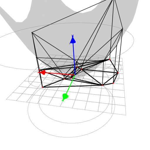
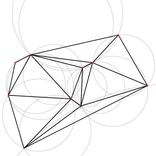
Refer to caption
Refer to caption
Figure 13: Bregman Delaunay triangulation as the projection of the convex polyhedron 𝒯𝒯\mathcal{T}.

We say that a Bregman sphere σ𝜎\sigma is empty if the open ball bounded by σ𝜎\sigma does not contain any point of 𝒮𝒮\mathcal{S}. The following theorem extends a similar well-known property for Delaunay triangulations whose proof (see, for example [10]) can be extended in a straightforward way to Bregman triangulations using the lifting map introduced in Section 3.2.

Theorem 12

The first-type Bregman sphere circumscribing any simplex of delF(𝒮)subscriptdel𝐹𝒮\mathrm{del}_{F}(\mathcal{S}) is empty. delF(𝒮)subscriptdel𝐹𝒮\mathrm{del}_{F}(\mathcal{S}) is the only triangulation of 𝒮𝒮\mathcal{S} with this property when 𝒮𝒮\mathcal{S} is in general position.

Several other properties of Delaunay triangulations extend to Bregman triangulations. We list some of them.

Theorem 13 (Empty ball)

Let ν𝜈\nu be a subset of at most d+1𝑑1d+1 indices in {1,,n}1𝑛\{1,\ldots,n\}. The convex hull of the associated points 𝐩isubscript𝐩𝑖\mathbf{p}_{i}, iν𝑖𝜈i\in\nu, is a simplex of the Bregman triangulation of 𝒮𝒮\mathcal{S} iff there exists an empty Bregman sphere σ𝜎\sigma passing through the 𝐩isubscript𝐩𝑖\mathbf{p}_{i}, iν𝑖𝜈i\in\nu.

The next property exhibits a local characterization of Bregman triangulations. Let T(𝒮)𝑇𝒮T(\mathcal{S}) be a triangulation of 𝒮𝒮\mathcal{S}. We say that a pair of adjacent facets f1=(f,𝐩1)subscript𝑓1𝑓subscript𝐩1f_{1}=(f,\mathbf{p}_{1}) and f2=(f,𝐩2)subscript𝑓2𝑓subscript𝐩2f_{2}=(f,\mathbf{p}_{2}) of T(𝒮)𝑇𝒮T(\mathcal{S}) is regular iff 𝐩1subscript𝐩1\mathbf{p}_{1} does not belong to the open Bregman ball circumscribing f2subscript𝑓2f_{2} and 𝐩2subscript𝐩2\mathbf{p}_{2} does not belong to the open Bregman ball circumscribing f1subscript𝑓1f_{1} (the two statements are equivalent for symmetric Bregman divergences).

Theorem 14 (Locality)

Any triangulation of a given set of points 𝒮𝒮\mathcal{S} (in general position) whose pairs of facets are all regular is the Bregman triangulation of 𝒮𝒮\mathcal{S}.

Let 𝒮𝒮\mathcal{S} be a given set of points, delF(𝒮)subscriptdel𝐹𝒮\mathrm{del}_{F}(\mathcal{S}) its Bregman triangulation, and 𝒯(𝒮)𝒯𝒮\mathcal{T}(\mathcal{S}) the set of all triangulations of 𝒮𝒮\mathcal{S}. We define the Bregman radius of a d𝑑d-simplex τ𝜏\tau as the radius noted r(τ)𝑟𝜏r(\tau) of the smallest Bregman ball containing τ𝜏\tau. The following result is an extension of a result due to Rajan for Delaunay triangulations [37].

Theorem 15 (Optimality)

We have delF(𝒮)=minT𝒯(𝒮)maxτTr(τ)subscriptdel𝐹𝒮subscript𝑇𝒯𝒮subscript𝜏𝑇𝑟𝜏\mathrm{del}_{F}(\mathcal{S})=\min_{T\in\mathcal{T}(\mathcal{S})}\max_{\tau\in T}r(\tau).

The proof mimics Rajan’s proof [37] for the case of Delaunay triangulations.

5.2 Bregman geodesic triangulations
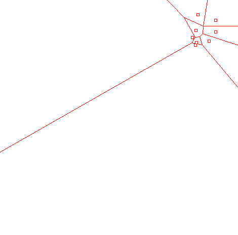
Refer to caption Refer to caption
(a) (b)
Figure 14: First-type Kullback-Leibler Bregman Voronoi diagram (a) obtained from the corresponding power diagram (b), and its associated dual regular triangulation rooted at gradient vertices (blue).

We have seen in Section 4.3 that the Bregman Voronoi of a set of points 𝒮𝒮\mathcal{S} is the power diagram of a set of balls superscript\mathcal{B}^{\prime} centered at the points of 𝒮superscript𝒮\mathcal{S}^{\prime} (Theorem 8). Write regF()subscriptreg𝐹superscript\mathrm{reg}_{F}(\mathcal{B}^{\prime}) for the dual regular triangulation dual to this power diagram. This triangulation444Applet at http://www.csl.sony.co.jp/person/nielsen/BVDapplet/ is embedded in 𝒳superscript𝒳\mathcal{X}^{\prime} and has the points of 𝒮superscript𝒮\mathcal{S}^{\prime} as its vertices (see Figure 14). The image of this triangulation by 1Fsuperscript1𝐹\mathbf{\nabla}^{-1}F is a curved triangulation whose vertices are the points of 𝒮𝒮\mathcal{S}. The edges of this curved triangulation are geodesic arcs joining two sites (see Section 3.3). We call it the Bregman geodesic triangulation of 𝒮𝒮\mathcal{S}, noted delF(𝒮)subscriptsuperscriptdel𝐹𝒮\mathrm{del}^{\prime}_{F}(\mathcal{S}) (see Figure 15).

Theorem 16

The Bregman geodesic triangulation delF(𝒮)subscriptsuperscriptdel𝐹𝒮\mathrm{del}^{\prime}_{F}(\mathcal{S}) is the geometric dual of the 1st-type Bregman Voronoi diagram of 𝒮𝒮\mathcal{S}.

Proof: We have, noting superscript\stackrel{{\scriptstyle*}}{{\equiv}} for the dual mapping, and using Theorem 8

vorF(𝒮)pow()reg()=F(delF(𝒮)).subscriptvor𝐹𝒮powsuperscriptsuperscriptregsuperscriptbold-∇𝐹subscriptsuperscriptdel𝐹𝒮\mathrm{vor}_{F}(\mathcal{S})\equiv\mathrm{pow}(\mathcal{B}^{\prime})\stackrel{{\scriptstyle*}}{{\equiv}}\mathrm{reg}(\mathcal{B}^{\prime})={{\bm{\nabla}}F}(\mathrm{del}^{\prime}_{F}(\mathcal{S})).

\square

Observe that delF(𝒮)subscriptsuperscriptdel𝐹𝒮\mathrm{del}^{\prime}_{F}(\mathcal{S}) is, in general, distinct from delF(𝒮)subscriptdel𝐹𝒮\mathrm{del}_{F}(\mathcal{S}), the Bregman Delaunay triangulation introduced in the previous section. However, when the divergence is symmetric, both triangulations are combinatorially equivalent and dual to the Bregman Voronoi diagram of 𝒮𝒮\mathcal{S}. Moreover, they coincide exactly when F𝐹F is the squared Euclidean distance.

Refer to caption Refer to caption Refer to caption
(a) Ordinary Delaunay (b) Exponential loss (c) Hellinger-like divergence
Figure 15: An ordinary Delaunay triangulation (a) and two Bregman geodesic triangulations for the exponential loss (b) and for the Hellinger-like divergence (c).

6 Applications

In this section, we give some applications related to computational geometry and machine learning.

6.1 Centroidal Bregman Voronoi diagrams and Lloyd quantization

Let 𝒟𝒟\mathcal{D} be a domain of 𝒳𝒳\mathcal{X} and p(𝐱)𝑝𝐱p(\mathbf{x}) be a density function defined over 𝒟𝒟\mathcal{D}. We define the Bregman centroid of 𝒟𝒟\mathcal{D} as the point 𝐜𝒟superscript𝐜𝒟\mathbf{c}^{*}\in\mathcal{D} such that 𝐜=argmin𝐜𝒟𝐱𝒟p(𝐱)DF(𝐱||𝐜)d𝐱\mathbf{c}^{*}=\mathrm{argmin}_{\mathbf{c}\in\mathcal{D}}\;\int_{\mathbf{x}\in\mathcal{D}}p(\mathbf{x})D_{F}(\mathbf{x}||\mathbf{c})\,\mathrm{d}\mathbf{x}. The following lemma states that the mass Bregman centroid of 𝒟𝒟\mathcal{D} is uniquely defined and independent of F𝐹F.

Lemma 11

The Bregman centroid of 𝒟𝒟\mathcal{D} coincides with the mass centroid of 𝒟𝒟\mathcal{D}.

Proof:

𝐜𝐱𝒟p(𝐱)DF(𝐱||𝐜)d𝐱\displaystyle\nabla_{\mathbf{c}}\int_{\mathbf{x}\in\mathcal{D}}p(\mathbf{x})\;D_{F}(\mathbf{x}||\mathbf{c})\,\mathrm{d}\mathbf{x} =\displaystyle= 𝐜𝐱𝒟p(𝐱)(F(𝐱)F(𝐜)𝐱𝐜,F(𝐜))d𝐱subscript𝐜subscript𝐱𝒟𝑝𝐱𝐹𝐱𝐹𝐜𝐱𝐜bold-∇𝐹𝐜differential-d𝐱\displaystyle\nabla_{\mathbf{c}}\int_{\mathbf{x}\in\mathcal{D}}p(\mathbf{x})\;(F(\mathbf{x})-F(\mathbf{c})-{\langle{\mathbf{x}-\mathbf{c}},{{{\bm{\nabla}}F}(\mathbf{c})}\rangle})\mathrm{d}\mathbf{x}
=\displaystyle= 𝐱𝒟p(𝐱)2F(𝐜)(𝐱𝐜)d𝐱subscript𝐱𝒟𝑝𝐱superscriptbold-∇2𝐹𝐜𝐱𝐜differential-d𝐱\displaystyle-\int_{\mathbf{x}\in\mathcal{D}}p(\mathbf{x})\;{{\bm{\nabla}^{2}F}}(\mathbf{c})(\mathbf{x}-\mathbf{c})\mathrm{d}\mathbf{x}
=\displaystyle= 2F(𝐜)(𝐱𝒟p(𝐱)𝐱d𝐱𝐜𝐱𝒟p(𝐱)d𝐱).superscriptbold-∇2𝐹𝐜subscript𝐱𝒟𝑝𝐱𝐱differential-d𝐱𝐜subscript𝐱𝒟𝑝𝐱differential-d𝐱\displaystyle-{{\bm{\nabla}^{2}F}}(\mathbf{c})(\int_{\mathbf{x}\in\mathcal{D}}p(\mathbf{x})\;\mathbf{x}\mathrm{d}\mathbf{x}-\mathbf{c}\int_{\mathbf{x}\in\mathcal{D}}p(\mathbf{x})\;\mathrm{d}\mathbf{x}).

Hence, 𝐜=𝐱𝒟p(𝐱)𝐱d𝐱𝐱𝒟p(𝐱)d𝐱superscript𝐜subscript𝐱𝒟𝑝𝐱𝐱differential-d𝐱subscript𝐱𝒟𝑝𝐱differential-d𝐱\mathbf{c}^{*}=\frac{\int_{\mathbf{x}\in\mathcal{D}}p(\mathbf{x})\;\mathbf{x}\mathrm{d}\mathbf{x}}{\int_{\mathbf{x}\in\mathcal{D}}p(\mathbf{x})\;\mathrm{d}\mathbf{x}}. \square

When 𝐱𝐱\mathbf{x} is a random variable following the probability density p(𝐱)𝑝𝐱p(\mathbf{x}), 𝐱𝒟p(𝐱)DF(𝐱||𝐜)d𝐱\int_{\mathbf{x}\in\mathcal{D}}p(\mathbf{x})\;D_{F}(\mathbf{x}||\mathbf{c})\,\mathrm{d}\mathbf{x} is called the distortion rate associated to the representative 𝐜𝐜\mathbf{c}, the optimal distortion-rate function 𝐱𝒟p(𝐱)DF(𝐱||𝐜)d𝐱\int_{\mathbf{x}\in\mathcal{D}}p(\mathbf{x})\;D_{F}(\mathbf{x}||\mathbf{c}^{*})\,\mathrm{d}\mathbf{x} is called the Bregman information, and 𝐜superscript𝐜\mathbf{c}^{*} is called the Bregman representative. The above result states that the optimal distortion rate exists and does not depend on the choice of the Bregman divergence, and that the Bregman representative 𝐜superscript𝐜\mathbf{c}^{*} is the expectation E(𝐱)𝐸𝐱E(\mathbf{x}) of 𝐱𝐱\mathbf{x}. This result extends an analogous result in the discrete case (finite point sets) studied in [6].

Computing a centroidal Bregman Voronoi diagram of k𝑘k points can be done by means of Lloyd’s algorithm [30]. We select an initial set of k𝑘k points. Then, we iteratively compute a Bregman Voronoi diagram and move the sites to the Bregman centroids of the corresponding cells in the diagram. Upon convergence, the output of the algorithm is a local minimizer of f((𝐩i,Vi),i=1,,k)=i=1k𝐱ViDF(𝐱||𝐩i)d𝐱f((\mathbf{p}_{i},V_{i}),i=1,\ldots,k)=\sum_{i=1}^{k}\int_{\mathbf{x}\in V_{i}}D_{F}(\mathbf{x}||\mathbf{p}_{i})\,\mathrm{d}\mathbf{x} , where {𝐩i}i=1ksuperscriptsubscriptsubscript𝐩𝑖𝑖1𝑘\{\mathbf{p}_{i}\}_{i=1}^{k} denotes any set of k𝑘k points of 𝒳𝒳\mathcal{X} and {Vi}i=1ksuperscriptsubscriptsubscript𝑉𝑖𝑖1𝑘\{V_{i}\}_{i=1}^{k} denotes any tesselation of 𝒳𝒳\mathcal{X} into k𝑘k regions. See [18] for a further discussion and applications of centroidal Voronoi diagrams.

6.2 ε𝜀\varepsilon-nets

Lloyd’s algorithm intends to find a best set of k𝑘k points for a given k𝑘k so as to minimize a least-square criterion. Differently, we may want to sample a compact domain 𝒟𝒳𝒟𝒳\mathcal{D}\subset\mathcal{X} up to a given precision while minimizing the number of samples. Instead of a least-square criterion, we define the error associated to a sample P𝑃P as error(P)=max𝐱𝒟min𝐩iPDF(𝐱||𝐩i){\rm error}(P)=\max_{\mathbf{x}\in\mathcal{D}}\,\min_{\mathbf{p}_{i}\in P}D_{F}(\mathbf{x}||\mathbf{p}_{i}). A finite set of points P𝑃P of 𝒟𝒟\mathcal{D} is an ε𝜀\varepsilon-sample of 𝒟𝒟\mathcal{D} iff error(P)εerror𝑃𝜀{\rm error}(P)\leq\varepsilon.

An ε𝜀\varepsilon-sample P𝑃P is called an ε𝜀\varepsilon-net if it satisfies the sparsity condition: max(DF(𝐩||𝐪),DF(𝐪||𝐩))>ε\max(D_{F}(\mathbf{p}||\mathbf{q}),D_{F}(\mathbf{q}||\mathbf{p}))>\varepsilon for any two points 𝐩𝐩\mathbf{p} and 𝐪𝐪\mathbf{q} in P𝑃P.

We will see how to construct an ε𝜀\varepsilon-net. For simplicity, we assume in the rest of the section that 𝒟𝒟\mathcal{D} is a convex polytope. Extending the results to more general domains is possible.

Let P𝒟𝑃𝒟P\subset\mathcal{D}, vorF(P)subscriptvor𝐹𝑃\mathrm{vor}_{F}(P) be the Bregman Voronoi diagram of P𝑃P and vorF|𝒟(P)subscriptvorconditional𝐹𝒟𝑃\mathrm{vor}_{F|{\mathcal{D}}}(P) be its restriction to 𝒟𝒟\mathcal{D}. Write V𝑉V for the set of vertices of vorF|𝒟(P)subscriptvorconditional𝐹𝒟𝑃\mathrm{vor}_{F|{\mathcal{D}}}(P). V𝑉V consists of vertices of vorF(P)subscriptvor𝐹𝑃\mathrm{vor}_{F}(P) and intersection points between the edges of vorF(P)subscriptvor𝐹𝑃\mathrm{vor}_{F}(P) and the boundary of 𝒟𝒟\mathcal{D}. The following lemma states that error(P)error𝑃{\rm error}(P) can be computed by examining only a finite number of points, namely the points of V𝑉V.

Lemma 12

error(P)=max𝐯Vmin𝐩iPDF(𝐱||𝐩i){\rm error}(P)=\max_{\mathbf{v}\in V}\,\min_{\mathbf{p}_{i}\in P}D_{F}(\mathbf{x}||\mathbf{p}_{i}).

Proof: Let 𝐱𝒟𝐱𝒟\mathbf{x}\in\mathcal{D}, 𝐩𝐱subscript𝐩𝐱\mathbf{p}_{\mathbf{x}} the point of P𝑃P closest to 𝐱𝐱\mathbf{x} and V𝐱subscript𝑉𝐱V_{\mathbf{x}} the associated cell of vorF|𝒟(P)subscriptvorconditional𝐹𝒟𝑃\mathrm{vor}_{F|{\mathcal{D}}}(P) (which contains 𝐱𝐱\mathbf{x}). V𝐱subscript𝑉𝐱V_{\mathbf{x}} is a bounded polytope whose vertices belongs to V𝑉V. Let 𝐰𝐰\mathbf{w} be the vertex of V𝐱subscript𝑉𝐱V_{\mathbf{x}} most distant from 𝐩𝐱subscript𝐩𝐱\mathbf{p}_{\mathbf{x}}. We have DF(𝐱||𝐩𝐱)DF(𝐰||𝐩𝐱)D_{F}(\mathbf{x}||\mathbf{p}_{\mathbf{x}})\leq D_{F}(\mathbf{w}||\mathbf{p}_{\mathbf{x}}). This is a consequence of the convexity of F𝐹F and of the fact that DF(𝐱||𝐩)D_{F}(\mathbf{x}||\mathbf{p}) is measured by the vertical distance between 𝐱^^𝐱\hat{\mathbf{x}} and H𝐩subscript𝐻𝐩H_{\mathbf{p}} (Lemma 1). \square

An ε𝜀\varepsilon-net of 𝒟𝒟\mathcal{D} can be constructed by the following greedy algorithm originally proposed by Ruppert in the context of mesh generation [39]. See also [20]. We initialize the sample set P0subscript𝑃0P_{0} with d𝑑d points of 𝒟𝒟\mathcal{D} lying at distance greater than ε𝜀\varepsilon from one another. Then, at each step, the algorithm looks for the point 𝐯isubscript𝐯𝑖\mathbf{v}_{i} of 𝒟𝒟\mathcal{D} that is the furthest (for the considered Bregman divergence) from the current set of samples Pisubscript𝑃𝑖P_{i}. By Lemma 12, this step reduces to looking at the vertices of vorF|𝒟(Pi)subscriptvorconditional𝐹𝒟subscript𝑃𝑖\mathrm{vor}_{F|{\mathcal{D}}}(P_{i}). If DF(𝐱||𝐯i)εD_{F}(\mathbf{x}||\mathbf{v}_{i})\leq\varepsilon, the algorithm stops. Otherwise, we take 𝐯isubscript𝐯𝑖\mathbf{v}_{i} as a new sample point, i.e. 𝐩i+1=𝐯isubscript𝐩𝑖1subscript𝐯𝑖\mathbf{p}_{i+1}=\mathbf{v}_{i}, we update the set of sample points, i.e. Pi+1=Pi{𝐩i+1}subscript𝑃𝑖1subscript𝑃𝑖subscript𝐩𝑖1P_{i+1}=P_{i}\cup\{\mathbf{p}_{i+1}\}, and insert 𝐩i+1subscript𝐩𝑖1\mathbf{p}_{i+1} in the Bregman Voronoi diagram of the sample points. Upon termination, the set of sample points Ptsubscript𝑃𝑡P_{t} satisfies the hypothesis of Lemma 12 and therefore Ptsubscript𝑃𝑡P_{t} is an ε𝜀\varepsilon-sample of 𝒟𝒟\mathcal{D}. Moreover, for any two points 𝐩𝐩\mathbf{p} and 𝐪𝐪\mathbf{q} of Ptsubscript𝑃𝑡P_{t}, we have DF(𝐩||𝐪)>εD_{F}(\mathbf{p}||\mathbf{q})>\varepsilon or DF(𝐪||𝐩)>εD_{F}(\mathbf{q}||\mathbf{p})>\varepsilon, depending on whether 𝐩𝐩\mathbf{p} has been inserted after or before 𝐪𝐪\mathbf{q}. Indeed, we only insert a point if its divergence to the points of the current sample is greater than ε𝜀\varepsilon. Hence, Ptsubscript𝑃𝑡P_{t} is an ε𝜀\varepsilon-net of 𝒟𝒟\mathcal{D}.

To prove that the algorithm terminates, we need the following lemma. Given a Bregman ball B(𝐜,r)𝐵𝐜𝑟B(\mathbf{c},r), we define the biggest Euclidean ball EB(𝐜,r)𝐸𝐵𝐜superscript𝑟EB(\mathbf{c},r^{\prime}) contained in B(𝐜,r)𝐵𝐜𝑟B(\mathbf{c},r) and the smallest Euclidean ball EB(𝐜,r′′)𝐸𝐵𝐜superscript𝑟′′EB(\mathbf{c},r^{\prime\prime}) containing B(𝐜,r)𝐵𝐜𝑟B(\mathbf{c},r).

Lemma 13

Let F𝐹F be a strictly convex function of class C2superscript𝐶2C^{2}, there are constants γsuperscript𝛾\gamma^{\prime} and γ′′superscript𝛾′′\gamma^{\prime\prime} (that do not depend on 𝐜𝐜\mathbf{c} nor on r𝑟r) such that r2γrsuperscript𝑟2superscript𝛾𝑟r^{\prime 2}\geq\gamma^{\prime}r and r′′2γ′′rsuperscript𝑟′′2superscript𝛾′′𝑟r^{\prime\prime 2}\leq\gamma^{\prime\prime}r.

Proof: According to Taylor’s formula, there exists a point 𝐭𝐭\mathbf{t} of the open segment 𝐱𝐜𝐱𝐜\mathbf{x}\mathbf{c} such that

F(𝐱)=F(𝐜)+𝐱𝐜,F(𝐜)+12(𝐱𝐜)T2F(𝐭)(𝐱𝐜).𝐹𝐱𝐹𝐜𝐱𝐜bold-∇𝐹𝐜12superscript𝐱𝐜𝑇superscriptbold-∇2𝐹𝐭𝐱𝐜F(\mathbf{x})=F(\mathbf{c})+{\langle{\mathbf{x}-\mathbf{c}},{{{\bm{\nabla}}F}(\mathbf{c})}\rangle}+\frac{1}{2}\;(\mathbf{x}-\mathbf{c})^{T}{{\bm{\nabla}^{2}F}}(\mathbf{t})(\mathbf{x}-\mathbf{c}).

Hence,

DF(𝐱||𝐜)=F(𝐱)F(𝐜)𝐱𝐜,𝐜=12(𝐱𝐜)T2F(𝐭)(𝐱𝐜),D_{F}(\mathbf{x}||\mathbf{c})=F(\mathbf{x})-F(\mathbf{c})-{\langle{\mathbf{x}-\mathbf{c}},{\mathbf{c}^{\prime}}\rangle}=\frac{1}{2}\;(\mathbf{x}-\mathbf{c})^{T}{{\bm{\nabla}^{2}F}}(\mathbf{t})(\mathbf{x}-\mathbf{c}), (14)

where 𝐭𝐭\mathbf{t} is a point of the open segment 𝐱𝐜𝐱𝐜\mathbf{x}\mathbf{c}.

Since F𝐹F is strictly convex, the Hessian matrix is positive definite (i.e., 𝐱T2F(𝐭)𝐱>0superscript𝐱𝑇superscriptbold-∇2𝐹𝐭𝐱0\mathbf{x}^{T}{{\bm{\nabla}^{2}F}}(\mathbf{t})\mathbf{x}>0 for all 𝐱𝐱\mathbf{x} in 𝒳𝒳\mathcal{X}), and the domain 𝒟𝒟\mathcal{D} being compact, there exist two constants ηsuperscript𝜂\eta^{\prime} and η′′superscript𝜂′′\eta^{\prime\prime} such that, for any 𝐲𝒟𝐲𝒟\mathbf{y}\in\mathcal{D}, 0<η′′2F(𝐲)η0superscript𝜂′′normsuperscriptbold-∇2𝐹𝐲superscript𝜂0<\eta^{\prime\prime}\leq||{{\bm{\nabla}^{2}F}}(\mathbf{y})||\leq\eta^{\prime}. If 𝐱𝐜2>2rη′′superscriptnorm𝐱𝐜22𝑟superscript𝜂′′\|\mathbf{x}-\mathbf{c}\|^{2}>\frac{2r}{\eta^{\prime\prime}} (Fröbenius matrix norm), we deduce from Equation (14) that DF(𝐱||𝐜)>rD_{F}(\mathbf{x}||\mathbf{c})>r. Therefore, B(𝐜,r)EB(𝐜,2rη′′)𝐵𝐜𝑟𝐸𝐵𝐜2𝑟superscript𝜂′′B(\mathbf{c},r)\subset EB(\mathbf{c},\sqrt{\frac{2r}{\eta^{\prime\prime}}}).

If 𝐱𝐜22rηsuperscriptnorm𝐱𝐜22𝑟superscript𝜂\|\mathbf{x}-\mathbf{c}\|^{2}\leq\frac{2r}{\eta^{\prime}}, we have using again Equation (14)

DF(𝐱||𝐜)η2𝐱𝐜2r.D_{F}(\mathbf{x}||\mathbf{c})\leq\frac{\eta^{\prime}}{2}\;\|\mathbf{x}-\mathbf{c}\|^{2}\leq r.

Therefore, EB(𝐜,2rη)B(𝐜,r)𝐸𝐵𝐜2𝑟superscript𝜂𝐵𝐜𝑟EB(\mathbf{c},\sqrt{\frac{2r}{\eta^{\prime}}})\subset B(\mathbf{c},r). \square

Let 𝐩𝐩\mathbf{p} and 𝐪𝐪\mathbf{q} be two points such that DF(𝐩||𝐪)=rD_{F}(\mathbf{p}||\mathbf{q})=r. Observing that EB(𝐩,r)EB(𝐩,𝐩𝐪)EB(𝐩,r′′)𝐸𝐵𝐩superscript𝑟𝐸𝐵𝐩norm𝐩𝐪𝐸𝐵𝐩superscript𝑟′′EB(\mathbf{p},r^{\prime})\subseteq EB(\mathbf{p},\|\mathbf{p}-\mathbf{q}\|)\subseteq EB(\mathbf{p},r^{\prime\prime}), we deduce from the above lemma that

γr𝐩𝐪γ′′rsuperscript𝛾𝑟norm𝐩𝐪superscript𝛾′′𝑟\sqrt{\gamma^{\prime}\,r}\leq\|\mathbf{p}-\mathbf{q}\|\leq\sqrt{\gamma^{\prime\prime}\,r} (15)

and

γγ′′DF(𝐩||𝐪)DF(𝐪||𝐩)γ′′γDF(𝐩||𝐪).\frac{\gamma^{\prime}}{\gamma^{\prime\prime}}D_{F}(\mathbf{p}||\mathbf{q})\leq D_{F}(\mathbf{q}||\mathbf{p})\leq\frac{\gamma^{\prime\prime}}{\gamma^{\prime}}D_{F}(\mathbf{p}||\mathbf{q}).

Another consequence of the lemma is that the volume of any Bregman ball of radius at least r>0𝑟0r>0, is bounded away from 0 (when F𝐹F is of class C2superscript𝐶2C^{2}). Hence, since 𝒟𝒟\mathcal{D} is compact, the algorithm cannot insert infinitely many points and therefore terminates. Moreover, the size of the sample output by the algorithm can be bounded, as stated in the next lemma. Write 𝒟ε={𝐱|𝐲𝒟,𝐱𝐲ε}superscript𝒟absent𝜀conditional-set𝐱formulae-sequence𝐲𝒟norm𝐱𝐲𝜀\mathcal{D}^{\leq\varepsilon}=\{\mathbf{x}|\ \exists\mathbf{y}\in\mathcal{D},\|\mathbf{x}-\mathbf{y}\|\leq\varepsilon\}.

Lemma 14

If F𝐹F is of class C2superscript𝐶2C^{2}, the algorithm terminates. If Ptsubscript𝑃𝑡P_{t} denotes the final set of sample points, we have |Pt|=O(vol(𝒟)ϵd/2)subscript𝑃𝑡𝑂vol𝒟superscriptitalic-ϵ𝑑2|P_{t}|=O\left(\frac{{\rm vol}(\mathcal{D})}{\epsilon^{d/2}}\right).

Proof: We have already shown that the algorithm terminates. Let Ptsubscript𝑃𝑡P_{t} be the set of points that have been inserted by the algorithm, excluding the initial set (of constant size). Let τ(𝐱)=inf{r:|EB(𝐱,r)Pt|2}𝜏𝐱infimumconditional-set𝑟𝐸𝐵𝐱𝑟subscript𝑃𝑡2\tau(\mathbf{x})=\inf\{r:|EB(\mathbf{x},r)\bigcap P_{t}|\geq 2\} and Bp=EB(𝐩,τ(𝐩)2)subscript𝐵𝑝𝐸𝐵𝐩𝜏𝐩2B_{p}=EB(\mathbf{p},\frac{\tau(\mathbf{p})}{2}), 𝐩Pt𝐩subscript𝑃𝑡\mathbf{p}\in P_{t}. It is easy to see that τ𝜏\tau is 1-Lipschitz and that the Euclidean balls Bpsubscript𝐵𝑝B_{p}, 𝐩Pt𝐩subscript𝑃𝑡\mathbf{p}\in P_{t} are disjoint. Let 𝐪𝐪\mathbf{q} be a point of Ptsubscript𝑃𝑡P_{t} closest to 𝐩𝐩\mathbf{p} : τ(𝐩)=𝐩𝐪𝜏𝐩norm𝐩𝐪\tau(\mathbf{p})=\|\mathbf{p}-\mathbf{q}\| and, as noticed above, max(DF(𝐩||𝐪),DF(𝐪||𝐩))>ε\max(D_{F}(\mathbf{p}||\mathbf{q}),D_{F}(\mathbf{q}||\mathbf{p}))>\varepsilon. Eq. 15 then implies that τ(𝐩)=𝐩𝐪γε𝜏𝐩norm𝐩𝐪superscript𝛾𝜀\tau(\mathbf{p})=\|\mathbf{p}-\mathbf{q}\|\geq\sqrt{\gamma^{\prime}\,\varepsilon}. Consider now the midpoint 𝐦𝐦\mathbf{m} of 𝐩𝐪𝐩𝐪\mathbf{p}\mathbf{q} and write 𝐭𝐭\mathbf{t} for the point of Ptsubscript𝑃𝑡P_{t} that minimizes DF(𝐦||.)D_{F}(\mathbf{m}||.). Since 𝒟𝒟\mathcal{D} is convex, 𝐦𝒟𝐦𝒟\mathbf{m}\in\mathcal{D} and, according to the definition of 𝐪𝐪\mathbf{q}, 𝐦𝐩𝐦𝐭norm𝐦𝐩norm𝐦𝐭\|\mathbf{m}-\mathbf{p}\|\leq\|\mathbf{m}-\mathbf{t}\|. Eq. 15 and the fact that Ptsubscript𝑃𝑡P_{t} is an ε𝜀\varepsilon-sample of 𝒟𝒟\mathcal{D} then yield 𝐦𝐭γ′′εnorm𝐦𝐭superscript𝛾′′𝜀\|\mathbf{m}-\mathbf{t}\|\leq\sqrt{\gamma^{\prime\prime}\,\varepsilon}. In summary, we have

γετ(𝐩)=𝐩𝐪2γ′′ε.superscript𝛾𝜀𝜏𝐩norm𝐩𝐪2superscript𝛾′′𝜀\sqrt{\gamma^{\prime}\,\varepsilon}\leq\tau(\mathbf{p})=\|\mathbf{p}-\mathbf{q}\|\leq 2\sqrt{\gamma^{\prime\prime}\,\varepsilon}. (16)

The right inequality shows that all the balls B𝐩subscript𝐵𝐩B_{\mathbf{p}}, 𝐩Pt𝐩subscript𝑃𝑡\mathbf{p}\in P_{t}, are contained in 𝒟ηsuperscript𝒟absent𝜂\mathcal{D}^{\leq\eta} where η=γ′′ε𝜂superscript𝛾′′𝜀\eta=\sqrt{\gamma^{\prime\prime}\,\varepsilon}. We can now bound the size of Ptsubscript𝑃𝑡P_{t}.

                  𝒟ηd𝐱τd(𝐱)subscriptsuperscript𝒟absent𝜂𝑑𝐱superscript𝜏𝑑𝐱\int_{\mathcal{D}^{\leq\eta}}\frac{d\mathbf{x}}{\tau^{d}(\mathbf{x})} 𝐩PtBp𝒟ηd𝐱τd(𝐱)absentsubscript𝐩subscript𝑃𝑡subscriptsubscript𝐵𝑝superscript𝒟absent𝜂𝑑𝐱superscript𝜏𝑑𝐱\geq\sum_{\mathbf{p}\in P_{t}}\int_{B_{p}\cap\mathcal{D}^{\leq\eta}}\frac{d\mathbf{x}}{\tau^{d}(\mathbf{x})}      (the balls Bpsubscript𝐵𝑝B_{p} have disjoint interiors)
𝐩Pvol(Bp𝒟η)(32τ(𝐩))dabsentsubscript𝐩𝑃volsubscript𝐵𝑝superscript𝒟absent𝜂superscript32𝜏𝐩𝑑\geq\sum_{\mathbf{p}\in P}\frac{{\rm vol}(B_{p}\cap\mathcal{D}^{\leq\eta})}{(\frac{3}{2}\tau(\mathbf{p}))^{d}}       (τ(𝐱)τ(𝐩)+𝐩𝐱32τ(𝐩)𝜏𝐱𝜏𝐩norm𝐩𝐱32𝜏𝐩\tau(\mathbf{x})\leq\tau(\mathbf{p})+\|\mathbf{p}-\mathbf{x}\|\leq\frac{3}{2}\;\tau(\mathbf{p}))
C3d|Pt|absent𝐶superscript3𝑑subscript𝑃𝑡\geq\frac{C}{3^{d}}\;|P_{t}|

where C=πpp!𝐶superscript𝜋𝑝𝑝C=\frac{\pi^{p}}{p!} if d=2p𝑑2𝑝d=2p and C=22p1(p1)!πp1(2p1)!𝐶superscript22𝑝1𝑝1superscript𝜋𝑝12𝑝1C=\frac{2^{2p-1}(p-1)!\,\pi^{p-1}}{(2p-1)!} if d=2p1𝑑2𝑝1d=2p-1.

Using again the Lipschitz property of τ𝜏\tau and Eq 16, we have for all 𝐱Bp𝐱subscript𝐵𝑝\mathbf{x}\in B_{p}

τ(𝐱)τ(𝐩)𝐱𝐩12τ(𝐩)12γε𝜏𝐱𝜏𝐩norm𝐱𝐩12𝜏𝐩12superscript𝛾𝜀\tau(\mathbf{x})\geq\tau(\mathbf{p})-\|\mathbf{x}-\mathbf{p}\|\geq\frac{1}{2}\;\tau(\mathbf{p})\geq\frac{1}{2}\,\sqrt{\gamma^{\prime}\,\varepsilon}

We deduce

|Pt|(6γ)d1Cεd/2𝒟η𝑑𝐱.subscript𝑃𝑡superscript6superscript𝛾𝑑1𝐶superscript𝜀𝑑2subscriptsuperscript𝒟absent𝜂differential-d𝐱|P_{t}|\leq\left(\frac{6}{\sqrt{\gamma^{\prime}}}\right)^{d}\;\frac{1}{C\varepsilon^{d/2}}\;{\int}_{\mathcal{D}^{\leq\eta}}\;\;d\mathbf{x}.

\square

A geometric object O𝑂O is said α𝛼\alpha-fat [7] if the ratio r+rsuperscript𝑟superscript𝑟\frac{r^{+}}{r^{-}} of the radius r+superscript𝑟r^{+} of the smallest ball enclosing O𝑂O over the radius rsuperscript𝑟r^{-} of the largest ball inscribed in O𝑂O is bounded by α𝛼\alpha: r+rαsuperscript𝑟superscript𝑟𝛼\frac{r^{+}}{r^{-}}\leq\alpha. Euclidean balls are therefore 111-fat, namely the fattest objects. It has been shown that considering the fatness factor for a set of objects yields in practice efficient tailored data-sensitive algorithms [7] by avoiding bad configurations of sets of skinny objects. A direct consequence of Lemma 13 is that Bregman balls (in fixed dimensions) are fat (i.e., α=O(1)𝛼𝑂1\alpha=O(1)) on any compact domain:

Corollary 3

For C2superscript𝐶2C^{2} Bregman generator functions, Bregman balls on any compact domain are fat.

Proof: Indeed, consider any Bregman ball defined on a compact domain for a C2superscript𝐶2C^{2} strictly convex and differentiable Bregman generator function F𝐹F. Its fatness α𝛼\alpha is upper bounded by γγ′′superscript𝛾superscript𝛾′′\sqrt{\frac{\gamma^{\prime}}{\gamma^{\prime\prime}}}, where γsuperscript𝛾\gamma^{\prime} and γ′′superscript𝛾′′\gamma^{\prime\prime} are the two constants (depending on F𝐹F and 𝒟𝒟\mathcal{D}) of Lemma 13. Recall that Lemma 13 considers concentric Euclidean balls ham sandwiching a Bregman ball, all centered at position 𝐜𝐜\mathbf{c}. We have αr+rr+r𝐜r𝐜+r𝐜=O(1)𝛼superscript𝑟superscript𝑟superscript𝑟superscriptsubscript𝑟𝐜superscriptsubscript𝑟𝐜superscriptsubscript𝑟𝐜𝑂1\alpha\leq\frac{r^{+}}{r^{-}}\leq\frac{r^{+}}{r_{\mathbf{c}}^{-}}\leq\frac{r_{\mathbf{c}}^{+}}{r_{\mathbf{c}}^{-}}=O(1) since r𝐜rsuperscriptsubscript𝑟𝐜superscript𝑟r_{\mathbf{c}}^{-}\leq r^{-} and r𝐜+r+superscriptsubscript𝑟𝐜superscript𝑟r_{\mathbf{c}}^{+}\geq r^{+}, where r𝐜+superscriptsubscript𝑟𝐜r_{\mathbf{c}}^{+} (respectively, r𝐜superscriptsubscript𝑟𝐜r_{\mathbf{c}}^{-}) denote the radius of the smallest enclosing (respectively, largest inscribed) Euclidean ball centered at 𝐜𝐜\mathbf{c}. The fatness property simply means that we can cover any Bregman ball by a constant number of (convex) Euclidean balls. \square

Thus, since Bregman balls are fat on compact domains, we can build efficient data-structures for point location with applications to piercing (geometric 00-transversal) and others, as described in [19].

6.3 VC-dimension, classification and learning

Some important classification rules rely on Voronoi diagrams; furthermore, the analysis of classification rules (complexity or statistical generalization) sometimes makes use of concepts closely related to Voronoi diagrams. Extending the rules and analyses to arbitrary Bregman divergences, with important related consequences (such as the eventual lost of convexity) is thus particularly interesting for classification, and we review here some notable consequences.

In supervised classification, we are generally interested in capturing the joint structure of 𝒳𝒳{\mathcal{X}} and a set of classes, {0,1}01\{0,1\} in the simplest case. For this objective, we build representations of concepts, i.e. functions that map 𝒳𝒳{\mathcal{X}} to the set of classes. A concept class {\mathcal{H}} is a set of concept representations h:𝒳{0,1}:𝒳01h:{\mathcal{X}}\rightarrow\{0,1\}; for example, should hh be a Bregman ball, it would classify 0 the points outside the ball, and 1 the points inside. Armed with these definitions, our supervised classification problem becomes the following one. A so-called target concept, c𝑐c, which is unknown, labels the points of 𝒳𝒳{\mathcal{X}}; we have access to its labeling throughout a sampling process: we retrieve examples (i.e., pairs (𝒙,c(𝒙))𝒙𝑐𝒙(\bm{x},c(\bm{x}))), independently at random, according to some unknown but fixed distribution 𝒟𝒟{\mathcal{D}} over the set {(𝒙,c(𝒙)):𝒙𝒳}conditional-set𝒙𝑐𝒙𝒙𝒳\{(\bm{x},c(\bm{x})):\bm{x}\in{\mathcal{X}}\}. The question is: what are the conditions on {\mathcal{H}} that guarantee the possibility to build, within reasonable time, some hh\in{\mathcal{H}} agreeing as best as possible with c𝑐c, with high probability? While the complexity requirement is usual in computer science, the fact that we require adequacy with high probability better than systematically is also a necessary requirement, as there is always the possibility of an extremely bad sampling that would prevent any efficient learning (e.g. we have drawn the same example all the time). In general, rather than directly sampling the domain, we work with a finite data set 𝒮𝒮{\mathcal{S}} of examples which is supposed to be sampled this way.

From the statistical standpoint, learning requires to find a good balance between the accuracy, i.e. the goodness-of-fit of hh as measured on 𝒮𝒮{\mathcal{S}}, and the capacity of {\mathcal{H}}, i.e. its ability to learn (or fit in generalization) the data with the smallest number of errors. Consider for example geometric figures in the plane and the “square” concept. Intuitively, an {\mathcal{H}} with too large capacity is like the person who picks a huge quantity of geometric figures including squares, memorizes each of them, and then rejects every square that would not exactly be in its collection (edge lengths, colors, etc.). An {\mathcal{H}} with too little capacity is like the lazy person who keeps as sole concept the fact that squares have four edges. Both extremal situations mean little generalization capabilities, but for different reasons.

There have been intensive lines of works on the measures of this capacity, and one of the most popular is the VC-dimension [17]. Informally, the VC-dimension of {\mathcal{H}} is the size of the largest dataset 𝒮𝒮\mathcal{S} for which {\mathcal{H}} shatters 𝒮𝒮\mathcal{S}, i.e. for which {\mathcal{H}} contains all the classifiers that could perform any of the 2|𝒮|superscript2𝒮2^{|\mathcal{S}|} possible labelings of the data. To be more formal, let Π(𝒮)={(h(𝒑1),h(𝒑2),,h(𝒑n))|h}subscriptΠ𝒮conditional-setsubscript𝒑1subscript𝒑2subscript𝒑𝑛\Pi_{{\mathcal{H}}}({\mathcal{S}})=\{(h(\bm{p}_{1}),h(\bm{p}_{2}),...,h(\bm{p}_{n}))\ |\ h\in{\mathcal{H}}\} denote the set of all distinct tuples of labels on 𝒮𝒮{\mathcal{S}} that can be performed by elements of {\mathcal{H}}. While it always holds that Π(n)2nsubscriptΠ𝑛superscript2𝑛\Pi_{{\mathcal{H}}}(n)\leq 2^{n}, the maximal n𝑛n for which Π(n)=2nsubscriptΠ𝑛superscript2𝑛\Pi_{{\mathcal{H}}}(n)=2^{n} is the VC-dimension of {\mathcal{H}}, VCdim()VCdim\textsc{VCdim}({\mathcal{H}}). The importance of the VC-dimension comes from the fact that it allows to bound the behavior of the empirical optimal classifier in a distribution-free manner [17]. In particular, if the VC-dimension is finite, the average error probability of the empirical optimal classifier tends to 0 when the size of the training data set increases. The following lemma proves that the VC-dimension of Bregman balls is the same as for linear separators, and this does not depend on the choice of F𝐹F.

Theorem 17

The VC dimension of the class of all Bregman balls BFsubscript𝐵𝐹B_{F} of dsuperscript𝑑\mathbb{R}^{d} (for any given strictly convex and differentiable function F𝐹F) is d+1𝑑1d+1.

Proof: We use the lifting map introduced in Section 3.2. Given a set 𝒮𝒮\mathcal{S} of points in dsuperscript𝑑\mathbb{R}^{d}, we lift them onto \mathcal{F}, obtaining 𝒮^d+1^𝒮superscript𝑑1\hat{\mathcal{S}}\in\mathbb{R}^{d+1}.

Let BFsubscript𝐵𝐹B_{F} be a Bregman ball and write σ𝜎\sigma for the Bregman sphere bounding BFsubscript𝐵𝐹B_{F}. From Lemma 5, we know that, for any 𝐩d𝐩superscript𝑑\mathbf{p}\in\mathbb{R}^{d}, 𝐩B𝐩𝐵\mathbf{p}\in B iff 𝐩^Hσ^𝐩superscriptsubscript𝐻𝜎\hat{\mathbf{p}}\in H_{\sigma}^{\downarrow}. For a given function F𝐹F, let Fsubscript𝐹\mathcal{B}_{F} denote the set of all Bregman balls, and let Fsubscript𝐹\mathcal{H}_{F} denote the set of all lower halfspaces of d+1superscript𝑑1\mathbb{R}^{d+1}. It follows from the observation above that \mathcal{B} shatters 𝒮𝒮\mathcal{S} iff \mathcal{H} shatters 𝒮^^𝒮\hat{\mathcal{S}}. Hence the VC dimension of \mathcal{B} over the sets of points of dsuperscript𝑑\mathbb{R}^{d} is equal to the VC dimension of \mathcal{H} over the sets of points of d+1superscript𝑑1\mathcal{F}\subset\mathbb{R}^{d+1}.

Since the points of 𝒮^^𝒮\hat{\mathcal{S}} are in convex position, they are shattered by \mathcal{H} iff the affine hull of their convex hull is of dimension strictly less than the dimension of the embedding space, i.e. d+1𝑑1d+1, which happens iff |𝒮|<d+2𝒮𝑑2|\mathcal{S}|<d+2. Indeed otherwise, the subset of vertices of any facet of the upper convex hull of 𝒮^^𝒮\hat{\mathcal{S}} cannot be obtained by intersecting 𝒮^^𝒮\hat{\mathcal{S}} with a lower halfspace (an upper halfspace would be required). Hence, the VC dimension of Bregman balls is at most d+1𝑑1d+1.

It is exactly d+1𝑑1d+1 since any set of d+1𝑑1d+1 points on \mathcal{F} in general position generates a d𝑑d-dimensional affine hull 𝒜𝒜\mathcal{A} that cannot be shattered by less than d+1𝑑1d+1 hyperplanes of 𝒜𝒜\mathcal{A}. The same result plainly holds for hyperplanes of d+1superscript𝑑1\mathbb{R}^{d+1} since we can associate to each hyperplane hh of 𝒜𝒜\mathcal{A} a hyperplane H𝐻H of d+1superscript𝑑1\mathbb{R}^{d+1} such that h=H𝒜𝐻𝒜h=H\cap\mathcal{A}. \square

This result does not fall into the general family of VC bounds for concept classes parameterized by polynomial-based predicates [23], it is mostly exact, and it happens not to depend on the choice of the Bregman divergence. This has a direct consequence for classification, which is all the more important as Bregman balls are not necessarily convex (see Figure 5). Because the capacity of Bregman balls is not affected by the divergence, if we fit this divergence in order to minimize the empirical risk (risk estimated on 𝒮𝒮{\mathcal{S}}), then there is an efficient minimization of the true risk (risk estimated on the full domain 𝒳𝒳{\mathcal{X}}), as well. There is thus little impact (if any) on overfitting, one important pitfall for classification, usually caused by over-capacitating the classifiers by tuning too many parameters.

Some applications of our results in supervised learning also meet one of the oldest classification rule: the k𝑘k-Nearest Neighbors (k𝑘k-NN) rule [22], in which a new observation receives the majority class among the set of its k𝑘k nearest neighbors, using e.g. k𝑘k-order Voronoi diagrams of 𝒮𝒮{\mathcal{S}} (Section 4.4). Various results establish upperbounds for the k𝑘k-NN rule that depend on the Bayes risk (the true risk of the best possible rule) [17]. The choice of the proximity notion between observations (it is often not a metric for complex domains) is crucial: if it is too simple or oversimplified, it degrades the k𝑘k-NN results and may even degrade Bayes risk as well; if it is too complicated or complexified, it may degrade the test results via the capacity of the rule. Searching for accurate “distance” notions has been an active field of research in machine learning in the past decade [42]. Our results on the linearity of the Bregman Voronoi diagrams essentially show that we can mix arbitrary Bregman divergences for heterogenous data (mixing binary, real, integer values, etc.) without losing anything from the capacity standpoint.

Range spaces of finite VC-dimensions have found numerous applications in Combinatorial and Computational Geometry. We refer to Chazelle’s book for an introduction to the subject and references wherein [15]. In particular, Brönnimann and Goodrich [13] have proposed an almost optimal solution to the disk cover algorithm, i.e. to find a minimum number of disks in a given family that cover a given set of points. Theorem 17 allows to extend this result to arbitrary Bregman ball cover (see also [21]).

7 Conclusion

We have defined the notion of Bregman Voronoi diagrams and showed how these geometric structures are a natural extension of ordinary Voronoi diagrams. Bregman Voronoi diagrams share with their Euclidean analogs surprisingly similar combinatorial and geometric properties. We hope that our results will make Voronoi diagrams and their relatives applicable in new application areas. In particular, Bregman Voronoi diagrams based on various entropic divergences are expected to find applications in information retrieval (IR), data mining, knowledge discovery in databases, image processing (e.g., see [24]). The study of Bregman Voronoi diagrams raises the question of revisiting computational geometry problems in this new light. This may also allow one to tackle uncertainty (’noise’) in computational geometry for fundamental problems such as surface reconstruction or pattern matching.

A limitation of Bregman Voronoi diagrams is their combinatorial complexity that depends exponentially on the dimension. Since many applications are in high dimensional spaces, building efficient data-structures is a major avenue for further research.

Acknowledgements

Frédéric Chazal, David Cohen-Steiner and Mariette Yvinec are gratefully acknowledged for their comments on this paper. The work by the second author has been partially supported by the project GeoTopAl (1555) of the Agence Nationale de la Recherche (ANR).

References

  • [1] S. Amari and H. Nagaoka. Methods of Information Geometry. Oxford University Press, ISBN 0-8218-0531-2, 2000.
  • [2] A. Ben-Hur, D. Horn, H. T. Siegelmann, and V. Vapnik Support Vector Clustering. Journal of Machine Learning Research, (2):125-137, 2001.
  • [3] F Aurenhammer. Power diagrams: Properties, algorithms and applications. SIAM Journal of Computing, 16(1):78–96, 1987.
  • [4] F. Aurenhammer and H. Imai. Geometric relations among voronoi diagrams. In 4th Annual Symposium on Theoretical Aspects of Computer Sciences (STACS), pp. 53–65, 1987.
  • [5] F. Aurenhammer and R. Klein. Voronoi Diagrams. In J. Sack and G. Urrutia (Eds), Handbook of Computational Geometry, Chapter V, pp. 201–290. Elsevier Science Publishing, 2000.
  • [6] A. Banerjee, S. Merugu, I. S. Dhillon, and J. Ghosh. Clustering with Bregman divergences. Journal of Machine Learning Research (JMLR), 6:1705–1749, 2005.
  • [7] M. de Berg, M. Katz, F. van der Stappen, and J. Vleugels. Realistic input models for geometric algorithms. Algorithmica 34:81-97, 2002.
  • [8] J.-D. Boissonnat and M. Karavelas. On the combinatorial complexity of Euclidean Voronoi cells and convex hulls of d𝑑d-dimensional spheres. In Proc. 14th ACM-SIAM Sympos. Discrete Algorithms (SODA), pp. 305–312, 2003.
  • [9] J.-D. Boissonnat, C. Wormser, and M. Yvinec. Anisotropic diagrams: Labelle Shewchuk approach revisited. In 17th Canadian Conference on Computational Geometry (CCCG), pp. 266–269, 2005.
  • [10] J.-D. Boissonnat and M. Yvinec. Algorithmic Geometry. Cambridge University Press, New York, NY, USA, 1998.
  • [11] J.-D. Boissonnat, C. Wormser, and M. Yvinec. Curved Voronoi diagrams. In J.-D. Boissonnat and M. Teillaud (Eds) Effective Computational Geometry for Curves and Surfaces, pp. 67–116. Springer-Verlag, Mathematics and Visualization, 2007.
  • [12] L. M. Bregman. The relaxation method of finding the common point of convex sets and its application to the solution of problems in convex programming. USSR Computational Mathematics and Mathematical Physics, 7:200–217, 1967.
  • [13] H. Brönnimann and M. T. Goodrich. Optimal set covers in finite VC-dimension. Discrete & Computational Geometry, 14(4):463–479, 1995.
  • [14] B. Chazelle. An optimal convex hull algorithm in any fixed dimension. Discrete Computational Geometry, 10:377–409, 1993.
  • [15] B. Chazelle. The Discrepancy Method. Cambridge University Press, Cambridge, U.K., 2000.
  • [16] I. Csiszár. Why least squares and maximum entropy? An axiomatic approach to inference for linear inverse problems. Ann. Stat., 19:2032–2066, 1991.
  • [17] L. Devroye, L. Györfi, and G. Lugosi. A Probabilistic Theory of Pattern Recognition. Springer, 1996.
  • [18] Q. Du, V. Faber, and M. Gunzburger. Centroidal Voronoi tesselations: Applications and algorithms. SIAM Review, 41:637–676, 1999.
  • [19] A. Efrat, M. J. Katz, F. Nielsen, and M. Sharir. Dynamic data structures for fat objects and their applications. Comput. Geom. Theory Appl., 15(4):215–227, 2000.
  • [20] Y. Eldar, M. Lindenbaum, M. Porat, and Y. Y. Zeevi. The farthest point strategy for progressive image sampling. IEEE Trans. on Image Processing, 6(9):1305–1315, 1997.
  • [21] G. Even, D. Rawitz, and S. Shahar. Hitting sets when the VC-dimension is small. Inf. Process. Lett., 95(2):358–362, 2005.
  • [22] E. Fix and J. L. Hodges. Discrimatory analysis, nonparametric discrimination. Technical Report TR-21-49-004, Rept 4, USAF School of Aviation Medicine, Randolph Field, TX, 1951.
  • [23] P.-W. Goldberg and M. Jerrum. Bounding the Vapnik-Chervonenkis dimension of concept classes parameterized by real numbers. Machine Learning, 18:131–148, 1995.
  • [24] M. Inaba and H. Imai. Geometric clustering models for multimedia databases. In Proceedings of the 10th Canadian Conference on Computational Geometry (CCCG’98), 1998.
  • [25] M. Inaba and H. Imai. Geometric clustering for multiplicative mixtures of distributions in exponential families. In Proceedings of the 12th Canadian Conference on Computational Geometry (CCCG’00), 2000.
  • [26] R. Klein. Concrete and Abstract Voronoi Diagrams, volume 400 of Lecture Notes in Computer Science. Springer, 1989. ISBN 3-540-52055-4.
  • [27] F. Labelle and J. R. Shewchuk. Anisotropic voronoi diagrams and guaranteed-quality anisotropic mesh generation. In Proc. 19th Symposium on Computational Geometry (SoCG), pages 191–200, New York, NY, USA, 2003. ACM Press.
  • [28] J. Lafferty. Additive models, boosting, and inference for generalized divergences. In Proc. 12th Conference on Computational learning theory, 125-133, 1999.
  • [29] D.-D. Le and S. Satoh. Ent-Boost: Boosting Using Entropy Measure for Robust Object Detection. In Proc. 18th International Conference on Pattern Recognition, pp. 602-605, 2006.
  • [30] S. P. Lloyd. Least squares quantization in PCM. IEEE Transactions on Information Theory, 28(2):129–136, 1982.
  • [31] P. McMullen. The maximum numbers of faces of a convex polytope. J. Combinatorial Theory, Ser. B, 10:179–184, 1971.
  • [32] F. Nielsen. Visual Computing: Geometry, Graphics, and Vision. Charles River Media/Thomson Delmar Learning, ISBN 1584504277, 2005.
  • [33] M. Teillaud O. Devillers, S. Meiser. The space of spheres, a geometric tool to unify duality results on voronoi diagrams. Technical Report No.1620, INRIA, 1992.
  • [34] K. Onishi and H. Imai. Voronoi diagram in statistical parametric space by Kullback-Leibler divergence. In Proc. 13th Symposium on Computational Geometry (SoCG), pages 463–465, New York, NY, USA, 1997. ACM Press.
  • [35] K. Onishi and H. Imai. Voronoi diagrams for an exponential family of probability distributions in information geometry. In Japan-Korea Joint Workshop on Algorithms and Computation, 1997.
  • [36] S. Pion and M. Teillaud. 3d triangulation data structure. In CGAL Editorial Board, editor, CGAL-3.2 User and Reference Manual. 2006.
  • [37] V. T. Rajan. Optimality of the Delaunay triangulation in dsuperscriptd\mathbb{R}^{\mbox{d}}. Discrete & Computational Geometry, 12:189–202, 1994.
  • [38] R. T. Rockafellar. Convex Analysis. Princeton University Press, Princeton, New Jersey, 1970.
  • [39] J. Ruppert. A Delaunay refinement algorithm for quality 2-dimensional mesh generation. J. Algorithms, 18:548–585, 1995.
  • [40] K. Sadakane, H. Imai, K. Onishi, M. Inaba, F. Takeuchi, and K. Imai. Voronoi diagrams by divergences with additive weights. In Proc. 14th Symposium on Computational Geometry (SoCG), pages 403–404, New York, NY, USA, 1998. ACM Press.
  • [41] M. Sharir. Almost tight upper bounds for lower envelopes in higher dimensions. Discrete Comput. Geom., 12:327–345, 1994.
  • [42] D. Randall Wilson and Tony R. Martinez. Improved heterogeneous distance functions. Journal of Artificial Intelligence Research, 1:1–34, 1997.