Matching NLO QCD computations with Parton Shower simulations: the POWHEG method
Abstract:
The aim of this work is to describe in detail the POWHEG method, first suggested by one of the authors, for interfacing parton-shower generators with NLO QCD computations. We describe the method in its full generality, and then specify its features in two subtraction frameworks for NLO calculations: the Catani-Seymour and the Frixione-Kunszt-Signer approach. Two examples are discussed in detail in both approaches: the production of hadrons in collisions, and the Drell-Yan vector-boson production in hadronic collisions.
GEF–TH–21/2007
1 Introduction
In the past two decades, next-to-leading order (NLO) QCD computations have become standard tools for phenomenological studies at lepton and hadron colliders. QCD tests have been mainly performed by comparing NLO results with experimental measurements, with the latter corrected for detector effects.
On the experimental side, leading order (LO) calculations, implemented in the context of general purpose Shower Monte Carlo (SMC) programs, have been the main tools used in the analysis. SMC programs include dominant QCD effects at the leading logarithmic level, but do not enforce NLO accuracy. These programs were routinely used to simulate background processes and signals in physics searches. When a precision measurement was needed, to be compared with an NLO calculation, one could not directly compare the experimental output with the SMC output, since the SMC does not have the required accuracy. The SMC output was used in this case to correct the measurement for detector effects, and the corrected result was compared to the NLO calculation.
In view of the positive experience with QCD tests at the NLO level, it has become clear that SMC programs should be improved, when possible, with NLO results. In this way a large amount of the acquired knowledge on QCD corrections would be made directly available to the experimentalists in a flexible form that they could easily use for simulations.
The problem of merging NLO calculations with parton shower simulations is basically that of avoiding overcounting, since the SMC programs do implement approximate NLO corrections already. Several proposals have appeared in the literature [1, 2, 3, 4] that can be applied to both and hadronic collisions, and two approaches [5, 6] suitable for annihilation. Furthermore, proposals for new shower algorithms, that should be better suited for merging with NLO results, have appeared in the literature (see refs. [7, 8, 9, 10, 11, 12]).
The MC@NLO
proposal [2] was the first one to give an acceptable
solution to the overcounting problem. The generality of the method has been
explicitly proven by its application to processes of increasing complexity,
such as heavy-flavour-pair [13] and
single-top [14] production.111 A complete list of
processes implemented in MC@NLO can be found at
http://www.hep.phy.cam.ac.uk/theory/webber/MCatNLO.
The basic idea of
MC@NLO is that of avoiding the overcounting by subtracting from the exact
NLO cross section its approximation, as implemented in the SMC
program to which the NLO computation is matched. Such approximated cross
section (which is the sum of what have been denoted in [2]
as MC subtraction terms) is
computed analytically, and is SMC dependent. On the other hand, the MC
subtraction terms are process-independent, and thus, for a given SMC, can be
computed once and for all. In the current version of the MC@NLO code, the
MC subtraction terms have been computed for HERWIG [15].
In general, the exact NLO cross section minus the MC subtraction terms does
not need to be positive. Therefore MC@NLO can generate events with
negative weights. For the processes implemented so far, negative-weighted
events are about 10–15% of the total. Their presence does not imply a
negative cross section, since at the end physical distributions must turn out
to be positive.
The features implemented in MC@NLO can be summarized as follows:
-
-
Infrared-safe observables have NLO accuracy.
-
-
Collinear emissions are summed at the leading-logarithmic level.
-
-
The double logarithmic region (i.e. soft and collinear gluon emission) is treated correctly if the SMC code used for showering has this capability.
In the case of HERWIG this last requirement is satisfied, owing to the fact that its shower is based upon an angular-ordered branching.
In ref. [4] a method, to be called POWHEG in the following (for Positive Weight Hardest Emission Generator), was proposed that overcomes the problem of negative weighted events, and that is not SMC specific. In the POWHEG method the hardest radiation is generated first, with a technique that yields only positive-weighted events using the exact NLO matrix elements. The POWHEG output can then be interfaced to any SMC program that is either -ordered, or allows the implementation of a veto.222All SMC programs compatible with the Les Houches Interface for User Processes [16] should comply with this requirement. However, when interfacing POWHEG to angular-ordered SMC programs, the double-log accuracy of the SMC is not sufficient to guarantee the double-log accuracy of the whole result. Some extra soft radiation (technically called vetoed-truncated shower in ref. [4]) must also be included in order to recover double-log accuracy. In fact, angular ordered SMC programs may generate soft radiation before generating the radiation with the largest , while POWHEG generates it first. When POWHEG is interfaced to shower programs that use transverse-momentum ordering, the double-log accuracy should be correctly retained if the SMC is double-log accurate. The ARIADNE program [17] and PYTHIA 6.4 [18] (when used with the new showering formalism), both adopt transverse-momentum ordering, in the framework of dipole-shower algorithm [19, 20, 21], and aim to have accurate soft resummation approaches, at least in the large limit (where is the number of colours).
A proof of concept for the POWHEG method has been given in ref. [22], for production in hadronic collisions. In ref. [23] the method was also applied to hadroproduction. Detailed comparisons have been carried out between the POWHEG and MC@NLO results, and reasonable agreement has been found, which nicely confirms the validity of both approaches. In ref. [24] the POWHEG method, interfaced to the HERWIG Monte Carlo, has been applied to annihilation, and compared to LEP data. The method yields better fits compared to HERWIG with matrix-element corrections. The authors of ref. [24] have also provided an estimate of the effects of the truncated shower, which turned out to be small.
In the present work we give a detailed description of the POWHEG method. Our aim is to provide all of the necessary formulae and procedures for its application to general NLO calculations. We first formulate POWHEG in a general subtraction scheme. Then, we illustrate it in detail in two such schemes: the Frixione, Kunszt and Signer (FKS) [25, 26] and the Catani and Seymour (CS) [27] one. The CS method has been widely used in the literature. On the other hand, the FKS method has already been used extensively in the MC@NLO implementations. Furthermore, the NLO cross sections for vector-boson and heavy-quark pair production used in the POWHEG implementations of refs. [22, 23] have a treatment of initial-state radiation that is essentially the same one used in FKS.
Our paper is organized as follows. In section 2 we summarize the general features of the NLO computations and of the subtraction formalisms. In section 2.4 all the details of the FKS subtraction method are given, and in section 2.5 the basic features of the CS approach are summarized.
In section 3 a general discussion of the inclusion of NLO corrections in a parton shower framework is given, together with a basic introduction of the POWHEG method.
In section 4 we go through all the details of the POWHEG method. The method is presented in general, and it is shown how to apply it within any subtraction framework. Thus, this section does not refer in particular to either the FKS or the CS method.
In section 4.4 we discuss the accuracy of the POWHEG approach in the resummation of soft-gluons effects. We show that, with an appropriate prescription for the evaluation of the running coupling used in POWHEG for the generation of radiation, one can easily obtain next-to-leading logarithmic (NLL) accuracy in soft-gluon radiation, provided the process in question has no more than three incoming or outgoing coloured partons at the Born level. If the Born process involves more than three coloured partons, there are left-over soft terms that are not correctly represented by POWHEG. We show, however, that with a modest modification of the algorithm one can also correctly resum these contributions at the level of the leading terms in a large expansion.
In section 5 the formulae needed for the explicit construction of a POWHEG in the FKS framework is given. The same is done in section 6 for the CS method.
Finally, in section 7 two simple examples are discussed in both the FKS and the CS framework, namely the production of hadrons in annihilation, and the production of a massive vector boson (or a virtual photon) in hadronic collisions.
This paper is considerably long, and it involves many technical details. The length is partly due to the fact that we deal with two subtraction methods. The reader may skip the one she/he is not interested in. The example sections are particularly long and pedantic. The reader may not be interested in reading all of them. Section 4.4 is technically complex, but it may be almost completely skipped on a first reading.
2 NLO computations
2.1 Generalities
In this section, we describe the general features of an NLO calculation for a generic hadron-hadron collision process. In lepton-hadron and lepton-lepton collisions, the treatment is similar, but simpler. For example, in the case of lepton-lepton collisions, the parton-distribution functions for the incoming particles are replaced by delta functions.
We consider processes, where the momenta of the particles satisfy the momentum conservation
| (1) |
where are the momentum fractions of the incoming partons, and the four-momenta of the incoming hadrons. In what follows, we also use the notation
| (2) |
to denote the momenta of the incoming partons. We define, as usual,
| (3) |
We denote by the set of variables
| (4) |
constrained by momentum conservation (eq. (1)), and by the on-shell conditions for final-state particles. We collectively denote by the squared matrix elements333 We always assume spin and colour sums and averages when needed, and the inclusion of the appropriate flux factor. relevant to the LO contributions to our process. The total cross section at leading order is given by
| (5) |
where is the parton luminosity444In this section we drop the parton flavours and the scale dependence in the luminosity, for ease of notation.
| (6) |
and
| (7) |
with the -body phase space
| (8) |
In case of leptons in the initial state, the corresponding parton distribution function in eq. (6) is replaced by .
The real contributions at the NLO arise from the tree-level squared amplitudes for the parton process, which we denote by . As before, we denote by the corresponding set of variables
| (9) |
constrained by momentum conservation and on-shell conditions.
The virtual contributions arise from the interference of the one-loop amplitudes times the LO amplitudes. We denote by the renormalized virtual corrections, that is, we assume that all ultraviolet divergences have already been removed by renormalization. These terms still contain infrared divergences. Therefore, they are computed in dimensions, and the divergences appear as and poles. The subscript (for “bare”) reminds us of the presence of infrared divergences in the amplitude.
In hadronic collisions, the complete cancellation of the initial-state collinear singularities is achieved by adding two counterterms, one for each of the incoming partons (, ), to the differential cross section. We denote them by and . The factorization counterterms are infrared divergent in four dimensions. Therefore, they are computed in dimensions, and the divergences appear as poles. To remind this fact, also in this case a subscript has been included in the notation.
The total NLO cross section is given by555The terms are present only for incoming hadrons. If one or both the incoming particles are leptons, the corresponding is zero.
| (10) | |||||
where
| (11) |
denotes configurations in which one of the final-state partons is collinear to one of the incoming partons. Thus, such configurations are effectively -body final-state ones, except for the energy degree of freedom of the parton collinear to the beam. We then write
| (12) | |||||
| (13) |
where is the fraction of momentum of the incoming parton after radiation. We can associate with the phase-space configuration an underlying -body configuration defined as
| (14) |
Thus, the values of in the underlying -body configuration are constrained by momentum conservation, and do not depend upon . We also define
| (15) | |||||
| (16) |
We now consider a generic observable , function of the final-state momenta. could be, for example, a product of theta functions describing a particular histogram bin for the distribution of some kinematic observable. Its expected value is given by
| (17) | |||||
where and are the expressions of the observable in terms of and final-state particle momenta, and , in the integrals, is the corresponding underlying -body configuration. We require that is an infrared-safe observable, and, furthermore, we require that the Born contribution in eq. (17) (i.e. the term proportional to ) is infrared finite (thus, for example, if our -body process corresponds to production, the observable must suppress the region where the jet is emitted at low transverse momentum). Under these assumptions, the real matrix elements contribution (i.e. the term proportional to ) is finite in the whole phase space , except for the regions that correspond to soft and collinear emissions. There, the divergences are integrable only in dimensions, and yield and poles. Furthermore the divergences of each term on the r.h.s. of eq. (17) cancel in the sum, and the total cross section is finite. Observe that the argument of in the last two terms on the right hand side of eq. (17) is set equal to rather than , owing to the fact that is an infrared-safe observable. The integrals in eq. (17) are usually too difficult to be performed analytically (because of the involved functional form of ) and, being divergent, they are not suited for numerical computations. For these reasons, different strategies have been proposed for the computation of observables in QCD. One of the most successful is the so-called subtraction method, pioneered in ref. [28], which we discuss in the next section.
2.2 Subtraction formalism
The subtraction formalism requires the definition of a set of functions , called real counterterms. Each is associated with a particular singular region, i.e. with a configuration that has either a final-state parton with four momentum equal to zero, or a final-state massless parton with momentum proportional to an initial-state or to another final-state massless parton. Furthermore, for each , a mapping666In some approaches, the counterterms are different from zero only in a finite neighborhood of the corresponding singular regions. In these cases, the mapping needs to be defined only there.
| (18) |
is defined that maps the -body configuration into a singular one.
The real counterterms and the mapping have the following property: for any infrared-safe observable , that vanishes fast enough if approaches two singular regions at the same time, the function
| (19) |
has at most integrable singularities in the space. Observe that the above condition does not always imply that
| (20) |
is also integrable. This is the case if the corresponding -body process has no singularities, like, for example, in production in hadronic collisions.
Each singular region is characterized by a different mapping, and, for this reason, we use the superscript on the tilded variables. For ease of notation, we use the following context convention: if an expression is enclosed in the subscripted squared brackets
| (21) |
we mean that all variables appearing inside have, when applicable, the superscripts corresponding to the subscript of the bracket. Thus we write
| (22) |
The form of the singular configurations differs according to the nature of the singular region. More specifically:
-
•
If is associated with a soft (S) region, the singular configuration has a final-state parton with null four-momentum.
-
•
If is associated with a final-state collinear singularity (FSC), the singular configuration has two massless final-state partons with parallel three-momenta.
-
•
If is associated with an initial-state collinear (ISC) singularity, the singular configuration has a massless outgoing parton with three-momentum parallel to the momentum of one incoming parton.
The mapping (18) must be smooth near the singular region, and it must become the identity there. In other words if, for instance, is associated with the FSC region where the particles and become collinear, we must have for . Notice that also the ’s of the configurations do not necessarily coincide with and for all -body configurations . On the other hand, they do coincide in the singular limit.
As in the case of the collinear configurations (eqs. (12) and (13)), we associate with each configuration an -body configuration , that we will call the underlying -body configuration
| (23) |
is obtained as follows:
-
•
If (i.e. it is a soft region), is obtained by deleting the zero momentum parton.
-
•
If (i.e. it is a final-state collinear region), is obtained by replacing the momenta of the two collinear partons with their sum.
-
•
If (i.e. it is an initial state collinear region), is obtained by deleting the radiated collinear parton, and by replacing the momentum fraction of the initial-state radiating parton with its momentum fraction after radiation.
In all the above cases, the final-state momenta are relabelled with an index that takes values in the range . Observe that, as a consequence of the procedure itemized above, the variables in are constrained by momentum conservation
| (24) |
Furthermore, for S or FSC regions, we have
| (25) |
This does not hold for ISC regions: in the direction, for example, we have
| (26) |
and the analogous one for the case of ISC in the direction.
We stress that the difference in our notation between the and is a minor one: the former has an unresolved parton, while in the latter all partons are resolved. On the other hand, it is necessary to introduce (together with the concept of underlying -body configuration), since it is formally the argument of Born-like matrix elements, and will play a central role in the development of the POWHEG formalism.
In the subtraction method one rewrites the contribution to any observable coming from real radiation in the following way
| (27) |
where . In this way, under the assumptions we have made about the counterterms, and the assumption that is an infrared-safe observable, the second term on the r.h.s. of eq. (2.2) is integrable in dimensions.
The first term on the r.h.s. of eq. (2.2) is divergent. In order to deal with it, we introduce, for each , the -phase space parametrization
| (28) |
and the corresponding phase-space element
| (29) |
In words, we parametrize the -phase space in terms of an -body phase space (obtained as described earlier), plus (three) more variables that describe the radiation process. The left-right arrow in eq. (28) indicates that the correspondence is one to one.777The correspondence needs only to be defined where the corresponding counterterm is non-vanishing. The range of the radiation variables in may depend upon . Furthermore, eq. (29) implicitly defines a Jacobian, possibly dependent upon , that we conventionally include into . We call the parametrization (28) the emission factorization.
We now distinguish two cases: the FSC+S case and the ISC one. In the former case we have
| (30) |
Defining
| (31) |
we can write the generic term in the first sum on the r.h.s. of eq. (2.2) as follows
| (32) |
In the ISC case, we cannot factor out the luminosity so easily, since . We define
| (33) |
which formally introduces the momentum fraction , and write
| (34) |
Notice that, owing to the delta function in eq. (33) we have
| (35) |
We also notice that the variables in the ISC regions can be identified with the variables in eqs. (12) and (13). In fact, the are integration variables, and can be identify with the ’s in eqs. (12) and (13). Furthermore, the variables are identical to the in eqs. (12) and (13), since those equations refer to a singular configuration, and (as we have remarked earlier) the mapping of eq. (18) is the identity in the singular region. It follows that the variables of eqs. (14) and (33) are identical. Hence, from eqs. (15) and (16), we obtain
| (36) |
(the factor in the second equation being due to the Jacobian for the change of variables ).
The choice of the counterterms in eq. (19) and of the mapping (18) should be such that the integrals in eqs. (31) and (33) are easily performed analytically in dimensions. In this way, the terms contain explicitly the divergences as poles in .
We now write eq. (17) as
| (37) | |||||
Notice that, in the last line, we have substituted for uniformity of notation. This is correct, since, as pointed out earlier, in the phase space of the collinear counterterms we have .
It turns out that it is always possible to write
| (38) |
where is finite in dimensions.888We point out that , although finite, may contain distributions associated with the soft region . The only remaining poles in are included in the last term of eq. (38), and have soft origin. It also turns out that in the quantity
| (39) |
all poles in cancel. With the notation
| (40) |
we mean that the argument between the brackets is evaluated for values of the phase-space variables equal to . Notice that the identification is possible, since refers to the underlying -body configuration, that must correspond to the Born term. Defining now the following abbreviations
| (41) |
equation (37) becomes
| (42) | |||||
and it is now suited to be integrated numerically, since all the integrals that appear in it are finite and can be evaluated in 4 dimensions.
2.3 Subtraction formalism using the “plus” distributions
The subtraction method naturally arises when results of NLO computations are expressed in terms of distributions in final-state variables. In order to illustrate this issue, we assume now for simplicity that there is just one singular region, and, in 4 dimensions, we describe the kinematics of the emitted parton (with momentum ) in the centre-of-mass (CM) frame of the incoming partons with the following variables
| (43) |
where , is the angle of the emitted parton relative to a reference direction (typically another parton), and is an azimuthal variable around the same reference direction. The singular regions (soft and collinear) are associated with and respectively. More generally, in dimensions, we can write
| (44) |
where
| (45) |
If we write
| (46) |
then is regular for and . The phase-space integral of is infrared divergent, and in dimensions (with ) the singular part of the integration is proportional to (see eq. (44))
| (47) |
In order to deal with the singularities, one uses the expansions
| (48) | |||||
| (49) |
with the usual definition of the prescription
| (50) | |||||
| (51) | |||||
| (52) |
Inserting eqs. (48) and (49) into (47), and defining , for ease of notation, we have
| (53) |
The first term on the r.h.s. of eq. (2.3), after integration in and , gives a contribution with the same structure as the virtual term, with which it is combined. Since this term arises from the factor, it can be easily obtained using the eikonal approximation for soft emissions in dimensions. The second term on the r.h.s. of eq. (2.3) is the contribution to proportional to the delta-function term in eq. (49), multiplied by the second and third term of eq. (48). It gives rise to terms that, in the case of final-state singularities, can also be integrated in and in , and yields terms of the same form of the virtual terms, with which it is combined. Also for this term it is not necessary to know in dimensions, since one can use the collinear approximation in the limit in order to obtain it. In the case of initial-state singularities, the same procedure gives terms of the same form of the collinear counterterms, with which they are combined. Finally, a term of the form
| (54) |
remains, where
| (55) |
Observe that the factor in front of eq. (55) cancels against the phase-space factor in eq. (54), and that has no singularities at and , so that distributions in and act on a regular function.
The procedure outlined in this section is fully general. It can be shown that, defining , one can rewrite eq. (42) in the form
| (56) | |||||
By handling the distributions in according to the prescriptions (50), (51) and (52), one automatically generates the real counterterms, provided the variables and appear in the phase-space parametrization. If more than one singular region is present, the real cross section is decomposed into a sum of terms, each of them having singularities in no more than one singular region. For each term, the phase space is parametrized in such a way that the variables and , appropriate to that particular singular region, are present.
The expression of a cross section in terms of distributions has sometimes the advantage that the associated projections are not uniquely fixed. In fact, one has the freedom to chose the integration variables other than and at one’s convenience. This amounts to choosing a different projection.
2.4 Frixione, Kunszt and Signer subtraction
In this section, we briefly review the FKS general subtraction formalism, proposed in refs. [25, 26], including a few modifications that have been introduced recently (see ref. [14]).
In FKS one expresses the cross section for the real-emission contribution as a sum of terms, each of them having at most one collinear and one soft singularity associated with one parton (called the FKS parton). The singular region associated with the final-state parton becoming soft or collinear to one of the incoming partons are labeled by , while those associated with final-state parton becoming soft or collinear to a final-state parton are labeled by the pair . For each singular region one introduces certain non-negative functions999The notation of refs. [25, 26] has been slightly changed here in order to simplify the discussion. Functions and of the present paper play the same role as and of ref. [26] respectively. of the -body phase space such that
| (57) |
We have two options for the range of the indices in the sums: we can let them range from 1 to (excluding only the possibility in the second sum), or we can assume that the and are zero (i.e. they are excluded from the sum) if the corresponding regions are not singular. For example, if refer to a quark and an antiquark of different flavour there cannot be a FSC singularity in this region, and we can set . Also, if is a gluon and is a quark, we may set to zero , since there is no soft singularity associated to becoming soft. Notice that if and are both gluons, both terms and appear in the sum, since there is a soft singularity for either parton becoming soft.
The function have the following properties
| (58) | |||
| (59) | |||
| (60) | |||
| (61) |
Thus, in a given soft region, (i.e. if parton is soft), all and with vanish, and eq. (57) is consistent with eq. (58). In a given initial-state collinear region, i.e. parton becomes collinear to an initial state parton, only is non-zero and equal to one, consistently with eq. (57). In a given final-state collinear region, i.e. if partons and are collinear, only and can differ from zero, their sum being 1, again consistently with eq. (57).
We now write
| (62) |
where
| (63) |
The terms give a divergent contribution (i.e. a contribution which has to be subtracted) only in the regions in which parton is soft and/or collinear to one of the initial-state partons, and the terms are divergent only in the regions in which parton is soft and/or collinear to final-state parton . Notice that if we have chosen the option of keeping all the functions different from zero, the and functions corresponding to non-singular regions are non-zero but finite.
Equations (58)–(61) are the only properties of the functions used in the analytical computations of refs. [25, 26]. Their actual functional forms, away from the infrared limits, are only relevant to numerical integrations.
After the -body cross section is decomposed as in eq. (62), FKS chooses a different parametrization of the -body phase space for each term, such that one can perform the necessary analytical and numerical integrations in an easy way. The key variables in the phase-space parametrization associated with are the energy of parton (directly related to soft singularities), and the angle between parton and one of the initial-state partons (directly related to initial-state collinear singularities). For , the energy of parton and the angle between parton and (related to a final-state collinear singularity) are chosen instead. Therefore, there are only two independent functional forms for phase spaces in FKS, one for initial- and one for final-state emissions.
In the following, we will need a further refinement of the FKS decomposition (eq. (57)). This is because, in FKS, the and collinear regions are both singled out by the functions. In POWHEG we will need sometimes to treat the two collinear regions separately. We thus introduce the notation
| (64) |
with the properties
| (65) |
that refine eq. (59). Eqs. (62) and (63) are modified accordingly.
2.4.1 The functions
In the original formulation of the FKS subtraction, the functions were defined as sets of functions. The different contributions to the real cross section, separated out in this way, corresponded to a partition of the phase space into non-overlapping regions. In the more recent calculation of single-top hadroproduction in MC@NLO [14], the functions were instead defined as smooth functions. In view of Monte Carlo implementations, step functions should be avoided as much as possible, and therefore we consider here the latter approach. We introduce the functions and , where , with the following properties
| (66) |
where energies and three-momenta are computed in the centre-of-mass frame of the incoming partons. A possible definition of the ’s is
| (67) | |||||
| (68) |
where is the angle between and , the angle between and , , and , are positive real numbers. Equations (67) and (68) can be easily expressed in terms of invariants using
| (69) |
which imply
| (70) | |||||
| (71) | |||||
| (72) |
We now introduce the quantity
| (73) |
and define
| (74) | |||||
| (75) |
where is a function such that
| (76) |
For example, one can define101010 In the original FKS formulation , which implies that defined in eq. (75) vanishes if . With such a choice, a proof was given in ref. [25] that all the infrared singularities are canceled by the FKS subtraction. We have checked that, if a smooth form for is adopted, this proof goes through unaltered by replacing in eq. (4.84) and (4.85) of ref. [25] with .
| (77) |
for some positive . Notice that the factor is necessary only if one considers both functions and (which is strictly necessary only if both and are gluons).
2.4.2 Contributions to the cross section
We introduce, for the FKS parton , the following variables
| (81) |
where is the angle of parton with the incoming parton , and is the angle of parton with parton . All variables are computed in the centre-of-mass frame of the incoming partons. The phase space for the and contributions is written in dimensions as
| (82) | |||||
where stands for either , or , . The transverse angular variables are relative to the collision axis, while are relative to the direction of parton . The singularities for , or are treated along the lines of section 2.3. The final expression in the FKS formalism results from the cancellation of the infrared singularities which emerge in the intermediate steps of the computation. It thus involves only non-divergent terms.
The contributions to the real-emission cross section, in the notation of eq. (56), are
| (83) |
where
| (84) | |||||
| (85) |
If we need to separate the and collinear regions, as discussed at the end of sec. 2.4, we have
| (86) | |||||
| (87) |
The distributions that appear in eqs. (84) and (85) are defined as follows
| (88) | |||||
| (89) |
The parameters , and must be chosen in the ranges and . The dependence they introduce in the -body contribution is exactly compensated by the same dependence in the -body contribution. In the POWHEG framework it is often convenient to use the maximal range of integration, and we will thus also use the notation
| (90) |
The parametrization of the -body phase space, appropriate to the integration of and , can be chosen as the version of equation (82), as suggested in the original FKS papers. This is however not necessary. Any parametrization of the phase space that allows a simple handling of the distributions is acceptable. This freedom is exploited in the present work, in order to simplify the formulation of the POWHEG method in the case of the contributions, where we make a choice of the azimuthal variables different from that of eq. (82).
We now consider the soft-virtual term in eq. (56). We define the set of all the parton labels for an -body process
| (91) |
The virtual contribution of eq. (37) is given by111111We stress that is the contribution to the cross section due to the interference of the virtual amplitude with the Born term. It thus includes the corresponding factor of 2.
| (92) |
where
| (93) |
Notice that, in the second sum on the r.h.s. of eq. (92), we sum over , and thus, since (as we show later) is symmetric, each term appears twice in the sum. The definition of the finite part depends upon the definition of the normalization factor , for which we have adopted the common choice of eq. (93), and from the regularization scheme, that we assume to be the standard conventional dimensional regularization (CDR).121212If we instead use the dimensional reduction (DR) scheme, we have , where, and , where is the number of colours. Finally, is the renormalization scale, and is an (arbitrary) physical scale that is factored out from the virtual amplitude in order to make the normalization dimensionless (thus depends upon and ).
The symbol denotes the flavour of parton , i.e. for a gluon, for a quark and for an antiquark. We define
| (94) | |||
| (95) | |||
| (96) |
In case is a colorless particle all the above quantities are zero.
The quantities , commonly referred to as the colour-correlated Born amplitudes, are defined in the following way
| (97) |
Here is the Born amplitude, and stands for the colour indices of all partons in . The suffix on the parentheses that enclose indicates that the colour indices of partons are substituted with primed indices in . Furthermore is the symmetry factor for identical particles in the final state, are the dimension of the colour representations of the incoming partons (3 for quarks and 8 for gluons), and are the number of spin states. The factor is the flux factor. We assume summation over repeated colour indexes ( for , , and ) and spin indices. For gluons , where are the structure constants of the algebra. For incoming quarks , where are the colour matrices in the fundamental representation (normalized as ). For antiquarks . It follows from colour conservation that satisfy
| (98) |
The soft-virtual term in eq. (56) is given by
| (99) |
The quantities and depend on the flavours and momenta of the incoming and outgoing partons. They are defined as follows
| (100) | |||||
| (101) | |||||
where is the energy of parton in the partonic centre-of-mass frame.
We finally report the expressions for the initial-state collinear remnants that appear in eq. (56). For each collinear singular configuration, relevant to the process, we have a term (and a corresponding one for ), where
| (102) | |||||
for a process in which an incoming parton of flavour splits into a parton (with fraction of the incoming momentum) that enters the Born process . The superscripts on denote the flavours of the incoming parton, and the dependence is to remind that the incoming momentum is rescaled. The distributions are defined as in eq. (88), with . The functions are the leading order Altarelli-Parisi splitting functions in dimensions, given by
| (103) | |||||
| (104) | |||||
| (105) | |||||
| (106) |
The distributions control the change of scheme in the evolution of parton distribution functions. They are defined in ref. [25], and equivalently, with the notation in ref. [27]. They are identically zero in .
2.5 Catani and Seymour subtraction
In this section we briefly review the general subtraction formalism proposed in ref. [27], called dipole subtraction. A dipole is defined by three partons: the emitted, the emitter and the spectator parton (the last two forming the dipole). In the dipole formulation, one given singular region receives, in general, contributions by several dipoles, differing among each other by the spectator parton. Thus, the counterterms are associated with dipoles, rather than singular regions. The maps of eq. (18) in the dipole formulation (that are summarized in section 6) are constructed in such a way that, in most cases, they affect only the momenta of the dipole partons, and all other momenta remain unchanged.131313The only exception is when the emitter and the spectator are the two incoming partons. The maps appropriate to the dipole subtraction will be discussed in section 6. These definitions, together with the definitions of the relative dipole counterterms (to be found in the original reference [27]) are necessary to define a POWHEG implementation. The last two missing ingredients are the soft-virtual term , and the collinear remnants . In this section we report explicitly the form of these terms, expressed in our notation.
For the soft-virtual contribution we obtain the following
| (107) |
Equation (107) has been obtained by a suitable manipulation of eqs. (C.27) and (C.28) of ref. [27]. The virtual term coincides with that of our eq. (92).
The collinear remnant is given by
| (108) | |||||
and the analogous one for . This formula is the translation in our notation of eq. (10.30) of ref. [27]. The definition of the functions , , and are given in appendix C of ref. [27].
In eq. (108), is the collinear remnant contribution for flavours of the incoming partons. Analogously, the superscripts in (and ) single out a given flavour combination for the incoming partons in the Born amplitudes and its colour-correlated components.
3 NLO with Parton Showers
3.1 Parton Shower Monte Carlo programs
A detailed discussion of the ideas upon which Shower Monte Carlo programs are based is beyond the scope of the present paper. The interested reader can find some pedagogical introductions e.g. in refs. [29, 30]. Here, we simply need to recall few basic features of SMC programs.
First, an MC starts from a kinematic configuration (“hard”) which is generated according to an exact LO computation. Usually such configuration is that of a partonic process. The final-state multiplicity is then iteratively increased, by letting each initial- and final-state parton branch into a couple of partons with a probability related to a Sudakov form factor. Thus, if at a given stage of the shower, the scattering process is described by partons, the algorithm decides with a certain probability whether branching is over at this stage, or further branchings will take place. In the latter case, one of the partons splits into a pair, generating an body final state. Thus, the algorithm defines a mapping
| (109) |
that is fully analogous to the mapping (28). Also in this case there is one mapping for each singular region, where the singular region is associated with the parton that undergoes the splitting. Observe that mappings defined in eq. (109) act non-trivially also on the momenta of the partons that do not undergo any splitting process. This is due to the fact that momentum conservation must be restored after branching, an operation that is usually referred to as “momentum reshuffling” in the SMC jargon. Also the value of the momentum fraction of the incoming partons may require readjustment, which leads to the fact that the value of the luminosity used for the cross-section computation does not correspond exactly to what one would have used if the -particle matrix element had been computed with standard methods. These readjustments usually amount to corrections beyond the (leading log) Monte Carlo accuracy, but should be analyzed carefully if one aims at NLO accuracy.
3.2 Including NLO corrections into Monte Carlo programs
The embedding of a NLO computation into an MC framework, as first clarified in ref. [2], aims at reaching NLO accuracy for inclusive observable, maintaining the leading logarithmic accuracy of the shower approach. This requires that the hardest emission that is generated has the correct distribution also far from the collinear directions, and that integrated quantities around the soft and collinear directions have NLO accuracy. This requirements are met in the MC@NLO approach by carefully tracing the differences of the MC simulation relative to the exact NLO one. The similarity of the mappings (109) and (28) are the starting point for this task. The shower algorithm is analyzed to determine its own approximate NLO structure in the subtraction framework, in order to determine unambiguously the difference with the exact NLO formulae.
In the POWHEG approach, one performs the generation of the hardest event with NLO accuracy, in a framework that does not depend upon the SMC’s shower algorithm. This is why it is fully independent from the SMC. Furthermore, the subsequent showers takes place at softer transverse momenta, and thus affects infrared-safe observables only at the next-to-next-to-leading order (NNLO). Thus, the matching problem considerably simplifies, since it no longer requires a detailed examination of the properties of the SMC.
3.3 POWHEG
In the POWHEG formalism, the generation of the hardest emission is performed first, using full NLO accuracy, and using the SMC to generate subsequent radiation. We give here a simple illustration of the method, ignoring, for the moment, the complications due to the presence of several singular regions in the NLO cross section. We begin by defining
| (110) | |||||
where we have assumed that all the , are expressed in terms of the barred variables. Next we introduce the Sudakov form factor141414Torbjörn Sjöstrand has pointed out to us that a similar Sudakov form factor is also used in PYTHIA for weak vector-bosons decay and production, in order to implement a matrix-element matching for the first emission in the shower, see refs. [30, 31].
| (111) |
The function should be equal, near the singular limit, to the transverse momentum of the emitted parton relative to the emitting one. The POWHEG cross section for the generation of the hardest event is then
| (112) |
where it is assumed that is parametrized in terms of and , and that values of are not allowed. The cross section (112) has the following properties:
-
•
At large it coincides with the NLO cross section up to NNLO terms.
-
•
It reproduces correctly the value of infrared safe observables at the NLO. Thus, also its integral around the small region has NLO accuracy.
-
•
At small it behaves no worse than standard Shower Monte Carlo generators.
Thus, it fulfills the requirement of the previous subsection for the inclusion of NLO corrections in an SMC.
As it stands, the POWHEG formula (112) can be used to feed a SMC program, that will perform all subsequent (softer) showers and hadronization. If the SMC is ordered in , we simply require that the shower is started with an upper limit on the scale equal to the of the POWHEG event. In case the SMC uses a different ordering variable, a problem arises, since the POWHEG cross section requires the emissions with higher to be suppressed in the SMC. This problem typically arises when interfacing POWHEG to angular ordered SMC’s. It is dealt with by vetoing emissions with larger in the shower, and by introducing vetoed truncated showers (see ref. [4]), that compensate for the fact that in angular ordered shower the hardest emission may not be the first.
Modern SMC programs, such as HERWIG and PYTHIA, have the capability of generating a vetoed shower. This is not the case for the vetoed truncated showers. We point out, however, that the need of vetoed truncated showers is not specific to the POWHEG method. As discussed in ref. [4], it also emerges naturally when interfacing standard matrix element calculations with parton shower, as in the approach of ref. [32]. At present, there is no evidence that the effect of vetoed truncated showers may have any practical important.
4 The POWHEG method
In order to implement the POWHEG method one must specify the separation of the singular regions, and the kinematics that associates a given -body singular region with an -body one. We discuss POWHEG in the framework of a generic subtraction formalism.
When one aims at the construction of an event generator, flavour should be carefully tracked, since different flavour structures always give rise to different events. We thus distinguish the contributions to the cross section also by their flavour structures, which are determined by the flavours of the incoming and outgoing partons. We call equivalent two flavour structures that differ only by a permutation of final-state partons. In particular, we label with the index the flavour structure of the -body processes and write and for the various Born and soft-virtual contributions.
We label with a particular contribution to the real cross section that is singular in only one singular region of integration and has a specific flavour structure. Thus, to each corresponds one and only one singular region. We then write
| (113) |
A similar separation also holds for the counterterms, so that they are also labelled by an index .
In the FKS case, for example, the contributions are obtained by first separating the real contribution into the sum of all its flavour components. For each flavour component, one constructs the functions, according to the procedure of section 2.4.1, and then multiplies it by the factors or . In the CS case, for each flavour component of the real contribution, one defines
| (114) |
where ranges in the set of dipoles with the same flavour structure.
To each contribution we can associate an underlying -body process, with a specific flavour structure. The association is performed as follows. If the singular region is collinear, the two collinear particles are merged into a single particle in such a way that flavour is conserved. In particular, a pair is merged into a , a pair is merged into a , and a () pair is merged into a (). If the singular region is soft, the soft gluon is removed. Observe that, for non singular limits (for example, in case two quarks, or a quark and an antiquark of different flavour become collinear, or in case a quark becomes soft) the flavour structure of the underlying -body process is undefined.
The factorization remnants also have a flavour structure. We label it with the index , and also for these configurations there is an underlying -body flavour structure. We call and the set of all values of the indices and that have the flavour structure of the underlying -body-configuration equal to .
We rewrite eq. (42) according to the notation of this section (making use of a straightforward extension of the context square brackets introduced in eq. (21))
| (115) | |||||
| (116) | |||||
| (117) | |||||
| (118) |
According to ref. [4], we now perform the following manipulation
| (119) | |||||
| (120) | |||||
| (121) |
The term of eq. (121) involves real radiation. All other terms (i.e. (116), (117) and (120)), have -body kinematics and, according to ref. [4], should be all lumped together into an -body kinematics term, that was called . However, we should now carefully distinguish the contributions to according to their flavour structure. We first rewrite eqs. (117), (120) and (121) in the following form
| (122) | |||||
| (123) | |||||
| (124) |
According to ref. [4], we can write the functions, one for each flavour configuration, as
| (125) | |||||
so that
| (126) |
and
| (127) | |||||
We now define the Sudakov form factors
| (128) |
Notice that the identification is a sensible one only if the underlying -body-process flavour structure of is equal to . In eq. (128), is a function of the kinematics variables that depends upon the particular singular region we are considering (its index is omitted in eq. (128) thanks to the context convention). For initial-state collinear singularities, we require that is proportional to the transverse momentum of the emitted parton with respect to the beam axis in the collinear limit. For final-state collinear singularities, assuming that the singular region corresponds to momenta and becoming collinear, we take as the (spatial) component of (or equivalently ) orthogonal to the sum . In the following we assume that the transverse momentum is computed in the CM frame of the colliding partons.
The factorization and renormalization scales adopted in the definition of , eq. (125), and in the definition of the Sudakov form factors, eq. (128), are different. In the definition of one adopts a choice that is appropriate to the Born cross section. In the Sudakov exponents one must instead adopt a scale of the order of . In section 4.4 we show that, with the above choice of scales, the Sudakov form factor of eq. (128) is equal, at least to the leading logarithmic (LL) level, to the DDT [33] Sudakov form factor, and that, in some cases, with a simple prescription, one can reach NLL accuracy.
The formula for the full POWHEG cross section is
| (129) | |||||
where, for ease of notation, we have dropped the argument in . The value introduced here is a lower cut-off on the transverse momentum, that is needed in order to avoid to reach unphysical values of the strong coupling constant and of the parton-density functions.
As discussed at the beginning of section 2.2, in case the -body cross section possesses singular regions, the observable should vanish fast enough if approaches two singular regions at the same time. Notice that, in the POWHEG cross section given in eq. (129), the observable function has disappeared, so that this restriction is no longer apparent in the formula. However, thanks to the partition of the different singular regions, it is sufficient to apply to the function a damping factor that suppresses the regions where the -body configuration becomes singular, in order to get a finite result. In this way, the POWHEG approach more closely resembles the standard Monte Carlo generators, where the hard leading-order matrix element for jet production is appropriately cut off in order to get a finite total cross section.
4.1 Transverse-momentum ordering
A word of caution has to be said with regard to the separation of the various singular contributions in POWHEG, in cases where the underlying -body cross section also possesses singular regions. In standard NLO calculations, these regions are avoided by simply requiring that the physical observables one computes should be finite for the -body term. In POWHEG, this requirement is in general not sufficient to guarantee consistency. We should also require that the of the generated radiation should not be harder than all the ’s associated with the underlying Born kinematics. More precisely, we should require that radiation with larger than the smallest of the underlying -body process should be suppressed. The separation of into contributions from the various singular regions achieves to some extent this purpose: is suppressed in any singular region different from . However, consistency with the treatment of soft singularities requires that the suppression should be based upon , rather than, for example, virtuality. Thus, in the FKS case (for example), a most appropriate choice for the is
| (130) | |||||
| (131) |
that correspond to the square of the transverse momentum to the power , rather than the form suggested in eqs (78) and (68).
4.2 NLO accuracy of the POWHEG formula
In ref. [4], it was argued that the POWHEG formula yields NLO accuracy for infrared-finite observables, and that subsequent showering by an SMC program does not spoil this conclusion. The second point is a simple consequence of the fact that no radiation with larger than that generated by POWHEG is allowed in the subsequent shower, and it requires no further discussion. We wish instead to address the first point more rigorously. In other words, we want to show in detail that formula (129), when used to compute an infrared-safe observable, yields the correct NLO accuracy. The reader that finds this conclusion already obvious can safely skip this section.
In order to ease the notation, we will drop the factor in the POWHEG formula, always assuming that this factor is present when there is real radiation.
where we have used the fact that . Furthermore, in the last term in the large curly bracket of eq. (132), small values in the integral are suppressed by the factor, and therefore we can replace and up to higher orders in . Equation (132) thus reduces to
| (134) | |||||
up to NNLO corrections. The restriction can now be dropped from the integration, its effect being suppressed by powers of , and formula eq. (134) is immediately found to agree with eq. (127), thus concluding our proof.
4.3 Practical implementation of the POWHEG formulae
The POWHEG cross section (eq. (129)) looks very complex, but, in fact, from a numerical point of view, it is quite easy to implement using few well-known Monte Carlo techniques.
4.3.1 Generation of the Born variables
To begin with, we must generate a Born-like configuration (a point in the space) and a value of the index , with a probability given by . The standard Monte Carlo technique used in this cases is the hit-and-miss procedure: one finds an upper bound to the cross section, generates randomly the phase-space point, and then accepts it with a probability equal to the ratio of the value of the cross section at the given point over the upper bound value. This technique is inadequate for our case, since each evaluation of the function requires an integration over the radiation variables. We thus proceed as follows. For each singular region, we parametrize the radiation variables in terms of a set of three variables in the unit cube, that we call . Similarly, the variable in the collinear remnants is parametrized in terms of one of these three variables, that we take to be . We then introduce the function
so that
| (136) |
and we define
| (137) |
There are computer programs that, after performing a single integration on a given function, can efficiently generate points in the integration range, distributed according to the integrand function. One such popular program is the BASES/SPRING package [34]. The adaptive Monte Carlo integration routine BASES performs the integration of the non-negative function, and stores the necessary intermediate results. The routine SPRING uses these information to generate unweighted events. In our case, one integrates the function in the full space using BASES. Then one generates points using SPRING. For each generated phase-space point, one chooses an value with a probability equal to . At this point, the values are discarded, and one has generated the values with probability proportional to . In essence, by doing a single -body phase-space integration, one is able to generate the Born configuration with reasonable efficiency.
As already pointed out, if the Born configuration possesses singular regions, the -body phase space should be suitably constrained, in order to avoid them. This is also the case in standard SMC programs: when one deals with cross sections with singular matrix elements, typically cross sections that include the production of a light parton, one specifies a transverse-momentum cut on its momentum, in order to get a finite total cross section. Alternatively, a weight should be attached to the function that suppresses the -body singular regions, so that the integral of is finite. Events are then generated using instead of , and a weight should be attached to each event. For example, in order to generate a sample of events, knowing that we will select jets with transverse energy greater than , we can restrict the Born events so that , being the transverse energy of the radiated parton. Alternatively, we weight with , attach the weight to the generated event, and unweight the events after the event sample (including cuts) is generated. The cut on the transverse energy of the associated jet should effectively cut off the events with low parton , so that the unweighting will be really possible.
4.3.2 Generation of the hardest-radiation variables
Given the Born kinematics , we must now generate the hardest-radiation configuration, characterized by , with , with probability
| (138) |
The Sudakov form factor can be written as
| (139) |
where
| (140) |
Under these conditions, the problem of generating the radiation variables according to eq. (138) can be reduced to the problem of generating them with probabilities
| (141) |
by using the highest-bid method, illustrated in appendix B. We are thus left with the problem of generating radiation variables according to eq. (141) for a fixed value of . This problem can be dealt with using the veto technique, illustrated in appendix A. In order to use this technique, we need a sufficiently simple upper bounding function
| (142) |
This can be found by taking the singular limit of the left hand side of eq. (142), that has, in general, a form suggested by the factorization theorem, and by elementary properties of the parton densities in the case of initial-state singular regions. Once the functional form of is guessed, its normalization is found by scanning the phase space.
Within a given subtraction method, one has typically two kinds of upper bounding functions: one for final-state radiation and one for initial-state radiation. In section 7 we illustrate explicit forms for in the FKS and CS frameworks, for both initial- and final-state radiation.
Notice that, in general, it is not necessary to separate out all regions in order to apply the veto method. In many cases several regions can be group together, thus simplifying the generation algorithm (see section 7).
4.4 Sudakov form factors and NLL soft gluon resummation
The purpose of the POWHEG method is to reach NLO accuracy for inclusive quantities, and leading logarithmic (LL) accuracy for exclusive final states. In this section we address the following question: to what extent we can do better than LL accuracy in the POWHEG framework? First of all, the POWHEG method deals with the hardest emission only. Subsequent emissions are handled by the shower Monte Carlo to which POWHEG is interfaced, and will have, in general, only LL accuracy. However, exclusive observables that are especially sensitive to the hardest emission will benefit from an improved POWHEG accuracy.
In this section, we show how to improve the logarithmic accuracy of POWHEG. We show that in many cases this improvement requires very minor adjustments of the POWHEG Sudakov form factor, and that in general, NLL accuracy at least in the large limit (where is the number of colours) should be easy to achieve. In all this section, for ease of notation, will denote the momentum of the soft gluon.
The results of this section can be summarized as follows:
-
1.
The POWHEG Sudakov form factor is accurate at the LL level, provided that the strong coupling constant and the parton density functions in the Sudakov exponent are evaluated at a scale of order .
-
2.
In case of processes involving no more than 3 coloured partons (in the initial or final state), NLL accuracy is achieved by replacing the strong coupling constant in the Sudakov exponent with
(143) where the , 1-loop expression of should be used. Furthermore, the parton densities in the exponent must be evaluated at a scale of order . The argument of in eq. (143) can also be taken equal to a function of the radiation variable that is of order in the soft or collinear limit, but becomes exactly equal to in the soft and collinear region.
-
3.
In case of processes involving more than 3 coloured partons, the procedure of item 2 is not sufficient to guarantee NLL accuracy. There are in fact soft (NLL) contributions that do exponentiate only in a matrix sense, so that, in order to deal with them using standard Monte Carlo techniques suited for the evaluation of ordinary exponential (like, for example, the veto method), one should diagonalize their colour structure.
-
4.
We will show that, for processes involving more than 3 coloured partons, the correct exponentiation of the soft (NLL) contributions discussed in item 3 can be easily recovered for the dominant terms in the large- limit.
In the rest of this section we will demonstrate the above points. We assume, in the following, that the reader is familiar with Sudakov resummation techniques, and in particular with ref. [35]. We also reassure the reader that, if she/he is willing to accept the above points, and is not interested in implementing the th point of the above list, the rest of this section can be safely skipped.
We begin by recalling the structure of Sudakov resummation of soft gluon effects in QCD, taking the notation and the results given in ref. [35]. One usually assumes that there are kinematic constraints that limit the emission of large transverse-momentum partons, called Sudakov weights in [35]. In the POWHEG Sudakov form factor, the constraint is given by the requirement that all radiation processes have transverse momentum less than a given , so that in our case. We now review the ingredients that build up the Sudakov resummation factors at NLL level. Radiation from a final-state massless parton carries a factor , given in eq. (10) of ref. [35]
| (144) |
where the function is defined in eq. (143). Furthermore,
| (145) |
where is a timelike vector, that we take to coincide with the time direction in the partonic CM system,151515In ref. [35] one is defined for each , Here, for simplicity, we identify all of them. and is the transverse momentum of relative to , defined as
| (146) |
in [35]. It corresponds in the soft-collinear limit to the transverse momentum of with respect to in the CM frame of the incoming partons. are appropriate combination of the Altarelli-Parisi splitting functions, defined in eq. (11) of ref. [35]. The soft (i.e. ) and collinear singularities in formula (144) give rise to logarithmic terms, with a structure (at the NLL level)
| (147) |
where is a reference scale of the order of the renormalization scale.
The logarithms arise in the following way. The collinear region of integration generates a . The soft region (i.e. ) also generates a , which arises from the terms in the functions. The NLL expansion of in powers of evaluated at a reference scale has the structure
| (148) |
and thus generates higher powers of logarithms. The coefficients in eq. (147) depend upon the coefficient of the term in , and upon the terms in eq. (148). The coefficients depend also upon the full form of , since non-soft, collinear terms can generate single-log contributions, and upon the terms in eq. (148). Furthermore, the term in also contribute to the coefficients. It arises from the singular part of the Altarelli Parisi splitting function, that has the form [36]
| (149) |
This relation holds for both the spacelike and timelike splitting function. The corresponding correction is associated with a collinear and soft singularity, and thus yields two logarithms. When combined with the terms of eq. (148) it gives rise to NLL contributions of order , , and so on. We notice that the expression in eq. (144) can be obtained from its own expansion
| (150) |
provided one replaces .
We now notice that the POWHEG Sudakov form factor has an exact expression of order in the exponent. Since formula (150) generates the dominant and terms, it must also be contained already in the POWHEG Sudakov exponent. It thus follows that, with the replacement of eq. (143) in the POWHEG Sudakov, we automatically include all LL and NLL terms of the factors. A similar reasoning holds for the resummation of initial state emissions161616In ref. [22] this case is discussed in details, in the framework of pair production in hadronic collisions., called factors in [35], and leads to the conclusion that, besides the replacement (143) one also needs to evaluate the parton densities in the Sudakov exponent at a scale of order , in order to achieve NLL accuracy.
The exponentiation of genuine soft, non-collinear interference contributions is more problematic. These contributions do not generally factorize in terms of the Born cross section. The real emission cross section in the soft limit has the well known structure
| (151) |
where are the colour correlated Born amplitude, defined in eq. (97), and is the Casimir invariant of the colour representation of parton . If parton is massless, also collinear singularities are present in formula (151). They can be separated out by exploiting the techniques used to derive the results in ref. [35]. Since that technique is illustrated in unpublished notes, in the following we sketch its main points. Defining , we have
| (152) |
In case of massless partons, for example, , we can separate out the collinear component
| (153) |
where is an arbitrary timelike vector. In the first term of the right hand side of eq. (153) there are no collinear singularities, since the factor in the square bracket vanishes when becomes collinear to . The second term in (153) is collinear, but being independent of gives a contribution of the form
| (154) |
factorized in terms of the Born cross section. Soft terms that factorize in terms of the Born amplitude are automatically included in the POWHEG framework, since the POWHEG exponent contains precisely the factor . Not so for the interference terms. We are thus left with terms of the form
| (155) |
We distinguish in the sum the massless and the massive case. The function in the POWHEG Sudakov exponent, eq. (128), could in principle be different for the various collinear regions of the soft parton. However, since formula (155) does not carry collinear singularities, the dominant integration region does not require any small angles. Under this condition, is of the order of , and at the single-logarithmic level one can replace
| (156) |
In other words, the integral in the radiation variables of the generic term of formula (155), with a theta function constraint , and defined relative to one generic yields a result of the form . If we replace the with the result will become , i.e. the logarithmically enhanced term remains the same.
The angular integration of the -dependent coefficients in eq. (155) yields (see Appendix C)
| (157) |
if , and
| (158) |
if . The NLL resummed Sudakov form factor associated with these soft emissions has the form
| (159) |
where corresponds to the expression for in eq. (9) of [35] (see also eqs. (14) and (15) there), excluding the factors.171717In ref. [35], only the case of massless partons is considered. Here is the Born matrix element, viewed as a complex vector in all its colour components. More precisely, is a tensor in colour space, carrying a colour index for each parton entering or leaving the amplitude. It thus spans a linear space, equipped with a sesquilinear product. The matrices can be seen as operators acting on this linear space. In facts, they act on the colour index of the th particle in . Thus the exponential is to be seen as the exponential of an operator in colour space. In ref. [35] the exponential is written as an energy-ordered one, to remind that this kind of exponentiation takes place because leading-log soft emission is dominated by energy-ordered graphs, where softer emission take place later (i.e. closer to the final-state lines). In fact, at NLL accuracy the ordering has no effect.
In the POWHEG formalism, the exponentiation of the soft interference terms has the form
| (160) |
since in POWHEG the ratio appears in the Sudakov exponent. This does not agree in general with eq. (159). There is, however, one important case in which it agrees, that is to say, when is an eigenstate of all the operators . In this case we can replace in the exponentials in eqs. (159) and (160) with their eigenvalues, and the two expressions become identical. It is also apparent that the are in this case all proportional to , and again we have complete factorization of the soft contribution in terms of the Born cross section. As discussed in ref. [35], if there are no more than 3 coloured partons entering or leaving the Born amplitude, it turns out that is always an eigenstate of the operator , for any . We conclude that, in this case, the prescription of eq. (143) is sufficient to guarantee NLL accuracy.
If there are more than 3 coloured partons in the amplitude, the standard POWHEG formula does not allow one to simply obtain full NLL accuracy. It should be very simple, however, to modify it in such a way that the interference soft terms are correctly resummed at NLL accuracy, at least as far as the dominant terms in the large- limit are concerned.
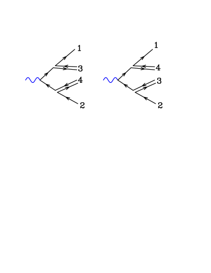
In the large- limit, the Born amplitude can be written as the sum of independent planar colour structures, that differ only by permutations of the external lines, as illustrated in fig. 1. We write
| (161) |
where the subscript stands for planar, and labels the different planar colour components. Observe that interference terms in the square of do not appear, since they give rise to non-planar structures, and are suppressed in the large limit. Soft emission factors give rise to leading contributions only if they act upon adjacent colour lines in the planar structures
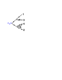
. In this case their effect amounts to a factor of , and they do not alter the colour connections of the Born planar amplitudes. It follows that
where with the notation we (somewhat imprecisely) indicate that we only consider adjacent colour lines for a given planar ordered amplitude. The last line of eq. (LABEL:eq:intpl) is similar to the form that appears in eq. (160), except that there is one term for each planar amplitude. This suggests how to implement it in the POWHEG framework. In section 4 we have introduced a classification of the Born contributions in terms of their flavour structure , and a classification of the real amplitude contributions in terms of their singularity regions and flavour structures . We need to extend this classification to include also the colour structure in the large limit. One simple way to do so is to compute and , the Born and real terms in the planar limit, for each of their given flavour structure. Then we define
| (163) |
so that
| (164) |
The labels and refer to the contribution of a given planar structure in the Born and Real contributions respectively. Next we must associate with each pair an underlying Born pair. As far as is concerned, the association is performed along the lines explained in section 4. For and , one proceeds as follows. If the singular region is soft, the Born planar colour structure is obtained by simply removing the soft gluon (and joining its colour lines) from the real emission colour structure. If the singular region is collinear, we need to show first that each has collinear singularities only for collinear particles that are nearby in its planar structure. This property follows from the fact that the ratio
| (165) |
has no collinear singularities, since the denominator is the large limit of the numerator, and therefore it has the same singular structure. It follows then, from the second equality in (163), that has the same collinear singularities of . Thus, since planar cross sections have collinear singularities only when nearby partons are collinear, has the same property. Joining the planar colour of nearby partons yields a valid Born planar colour configuration. We now introduce
| (166) |
and the corresponding POWHEG Sudakov form factor
| (167) |
that should correctly generate large angle soft radiation in the large limit. Equations (166) and (167) certainly satisfy the formula (LABEL:eq:intpl) for the soft interference terms in the large limit. We must still show that collinear singularities are treated correctly for all , i.e. that formula (167) is equivalent to formula (128) in the collinear regions. This is the case if
| (168) |
in the collinear region. Using eqs. (163) we write
| (169) |
The second term on the r.h.s. of eq. (169) yields 1 in the collinear limit. In fact, it is easy to convince oneself that, in this limit, both its numerator and denominator yield the (planar) Altarelli Parisi splitting kernel, that simplifies in the ratio. Thus becomes independent in this limit, and the overall factor can be summed in , to yield back .
We conclude this section by reminding the reader that the importance of the inclusion of soft-interference terms should not be overemphasized at this stage. After all, the POWHEG formula in eq. (160) differs from formula (159) only starting at order . It is thus unlikely that these terms will have important effects in a full POWHEG implementation. Nevertheless, if one wants to assess their importance, one can, to begin with, implement their large resummation and study its impact.
4.5 Interfacing POWHEG to an SMC
The POWHEG algorithm generates the kinematics and flavour configuration of the hardest-emission event. The event should be fed into a SMC using the Les Houches Interface for User Processes [16] (LHIUP from now on). In particular, one should require that no events harder than the one generated by POWHEG should be generated by the SMC. This is achieved by setting the variable SCALUP of the LHIUP equal to the of the POWHEG event. The LHIUP specifies how to pass the kinematics and flavour structure of the hard event to the SMC.
4.5.1 Colour assignment
The LHIUP also requires that the colour connections of the hard event (in the large limit) should also be specified. POWHEG does not, in general, generate these large- colour structures. They are needed (and can be generated) only if one wishes to reach large- NLL accuracy of the Sudakov form factor, in events with more than 3 coloured partons at the Born level, as discussed in section 4.4. If this is not the case, the generation of the colour configuration should be performed after the POWHEG event has been generated. Here we illustrate two acceptable ways to perform colour assignment. The first (and simpler) approach is the following:
-
•
Generate the POWHEG event in the standard way.
-
•
Compute the different (planar) colour contributions to the Born cross section, at the kinematics of the generated underlying Born configuration.
-
•
Pick an underlying Born colour configuration, with a probability proportional to the corresponding (planar) colour Born contribution.
-
•
If no radiation has been generated, this is the colour structure of the event.
-
•
If radiation has been generated, POWHEG has also generated a index, specifying a singular region. In this case we always assume that the emitted parton is (planar) colour-connected to the emitter. This fully specifies the planar colour structure of the event.
This method only requires the calculation of the planar colour-structures of the Born term. In the second method (which is usually implemented in MC@NLO) one computes all the planar colour contributions to , and chooses the colour configuration with a probability proportional to the corresponding contribution.
5 POWHEG in the Frixione, Kunszt and Signer framework
In this section we construct a mapping from the phase space to the barred and radiation variables of eq. (28) (and its corresponding inverse mapping) for the two kinds of singular regions (initial state) and (final state), that is compatible with the FKS subtraction method. These is the only missing ingredients one needs to construct a POWHEG generator in the FKS framework.
We stress that the mapping that we propose is not the only possible one. In practical examples one may find convenient to depart from this approach. It is however fully general, and as such it may be implemented once and for all in a computer code to be used for all processes.
5.1 Initial-state singularity
5.1.1 Radiation and barred variables
We first show how to construct the underlying Born (i.e. the barred variables) and the three radiation variables from the kinematics, for the case of the initial-state singularity region.
Without loss of generality, we assume that the FKS parton is the th one, so that the mapping from to () does not requires a relabeling of the momenta. In the FKS formulation, is a function of , and (see eq. (43)), so that, in the centre of mass of the colliding partons, i.e. the CM of the system, we have
| (170) |
We take , and as the radiation variables for the singular region, and obtain
| (171) |
We introduce the momentum
| (172) |
and construct a longitudinal boost (longitudinal with respect to the incoming beams) such that has zero longitudinal component. Notice that is unique, being given by a longitudinal boost with boost angle equal to minus the rapidity of . Then we construct a transverse boost such that has zero transverse momentum. We then define the barred momenta as
| (173) |
and define
| (174) |
We notice that, by construction, and have the same invariant mass and rapidity. We now define and in such a way that
| (175) |
An explicit expression for and is easily obtained, by using the fact that and have the same invariant mass and rapidity. We get
| (176) |
and
| (177) |
Observe that we always have and . The phase space can be rewritten as follows
| (178) | |||||
where we have used the boost invariance of the -body phase space. Thus, from eq. (29) we obtain
| (179) |
5.1.2 Inverse construction
We describe now the construction of the full -particle phase space, given the barred variables and the radiation variables , and . Using eq. (170) we fully construct . Inverting eq. (176), we have
| (180) |
The range for the variable is now restricted by the requirement that both and be less than 1. This gives
| (181) |
with
| (182) | |||||
From and we can construct , and summing the barred momenta, according to eq. (174), we can compute
| (183) |
The four vectors and have the same invariant mass and rapidity by construction, since the relation between the and the was obtained precisely from these conditions. We then construct the boost such that has zero rapidity. We will also have that has zero rapidity. Then we compute the transverse boost such that
| (184) |
Finally, the momenta , are obtained as
| (185) |
This completes the construction of the -body phase space, starting from an underlying Born configuration and the three radiation variables.
5.2 Final-state singularity
5.2.1 Radiation and barred variables
In this section, we show how to construct the underlying Born and the three radiation variables, given the variables, in the case of final-state singularity. We assume, without loss of generality, that the singular region is associated with partons and , that is, the th parton becoming collinear to the th parton, or becoming soft.
Our mapping is constructed in such a way that
| (186) |
Thus, the partonic CM frame of the final-state -particle system coincides with the CM frame of the barred momenta , and we work in this frame from now on. In this section (and only here), we need to introduce a short-hand notation for the modulus of the space component of a four-vector in the CM frame
| (187) |
We then define
| (188) |
and, in the CM frame, we have
| (189) |
Introducing the four momentum
| (190) |
we define the radiation variables as
| (191) |
where is an arbitrary direction that serves as origin for the azimuthal angle of around , and “” is the cross vector product. The notation denotes the angle between and . Thus, is the azimuth of the vector around the direction . Notice that only and correspond exactly to FKS variables, since the FKS azimuth is usually defined with respect to rather than . We prefer the choice (191) because we want to defined the mapping in such a way that the direction (rather than the one) is preserved. Our choice, however, makes only irrelevant differences in the FKS formalism, since the real-emission cross section has singular distributions only in the variables and .
We introduce the recoil four-momentum and mass
| (192) |
We have
| (193) |
We construct a boost along the direction, such that the 4-momentum is light-like, that is to say
| (194) |
The boost velocity is easily computed
| (195) |
Since , and , is positive and smaller than one. Thus, the boost always exists. We define the barred momenta as
| (196) |
so that they clearly satisfy momentum conservation
| (197) |
In order to obtain , we write the -body phase space as
| (198) | |||||
where, in the last equality, using eq. (190), we have traded for as independent variable. We thus have now
| (199) |
We identify the phase space in eq. (198) with the phase space written in terms of the barred and radiation variables, multiplied by a Jacobian factor
| (200) | |||||
We work out this equality simplifying common factors, until we obtain an expression for . We consider the barred and radiation variables to be functions of the unbarred variables. First of all, we remind that and have the same direction. We thus make the replacements
| (201) |
and cancel the common factor on both sides of eq. (200). Boost invariance of the phase-space elements and of the four-dimensional delta function also guarantees that
| (202) |
In fact, , , and are functions of and only, while depend upon via the boost , that depends only upon and . Furthermore, according to (196),
| (203) |
so that eq. (202) is implied by boost invariance. The members of eq. (202) can thus be divided out on both sides of eq. (200). Performing also the replacement
| (204) |
where is the angle between and , on the left hand side of eq. (200), we can also divide out . We are left with the identity
| (205) |
and, thus, we just need to express and in terms of and , at fixed , and compute the Jacobian of this two-variable transformation. The following sequence of relations give and as functions of and (at fixed )
| (206) |
Thus
| (207) |
where
| (208) |
and we get
| (209) |
so that
| (210) |
5.2.2 Inverse construction
In this section, we describe the construction of the full -particle phase space, given the barred variables and the radiation variables , and . We immediately have
| (211) |
The absolute value of the three-momentum of must instead be obtained by solving the equation for the energy conservation
| (212) |
where
| (213) |
and , according to eqs. (192), (196) and (197), is given by
| (214) |
Under the obvious condition
| (215) |
there is one and only one (positive) solution of eq. (212)
| (216) |
Having specified the size of , we construct the vectors and in such a way that their vector sum is parallel to , and that the azimuth of relative to (the given reference direction) is . Having constructed and , we can define and find . We can now compute according to eq. (195), and obtain
| (217) |
Thus, the inverse mapping exists provided
| (218) |
and it is always unique.
6 POWHEG in the Catani and Seymour framework
The separation of into singular components may require particular attention. First of all, if one uses the formula
| (219) |
a problem may arise due to zeros in the denominator (in fact, the CS counterterms are not necessarily positive). We have not tried to prove that this can really happen. However, the problem is easily solved by using instead (for example)
| (220) |
In case the -body cross section possesses singular regions, as discussed at the beginning of section 2.2, a further problem may arise. Formula (219) may not be adequate to partition the different singular components of . This is better seen with an example. Consider the production process. The -body process corresponds to a final state, where is a light parton, and the -body process corresponds to a final state, where and are light partons. Consider now the counterterm corresponding to becoming collinear to an initial-state parton. It is proportional to the underlying parton cross section. It is therefore also singular when becomes collinear to an initial-state parton, since the cross section is singular in this limit. In standard NLO calculation, an infrared-safe observable , that vanishes when two singular regions are approached at the same time, suppresses the singular regions of the underlying Born process in the counterterm (see eq. (19)). This problem is easily solved by writing
| (221) |
where is a positive function that vanishes when its argument approaches an -body singular configuration. We again have
| (222) |
and now is singular only in the region.
If one wishes to enforce transverse-momentum ordering (see sec. 4.1), one can first separate as in eqs. (62) and (63), using the functions defined in eqs. (75) and (80), with the functions defined as in eqs. (130) and (131). The contributions to corresponding to a given singular region can then be separated according to each possible spectator using a formula similar to eq. (221).
We now discuss the various dipole configurations of the CS approach. We use the notation introduced in ref. [27], slightly modified in order to be consistent with the notation of the rest of this paper.
6.1 Final-state singularity with final-state spectator
6.1.1 Radiation and barred variables
The labels denote the radiator, the emitted, and the spectator partons respectively. Without loss of generality, we assume that the radiated parton is the th parton. We introduce the variable , that is zero in the soft and collinear limit,
| (223) |
The barred momenta, are defined as follows
| (224) | |||||
| (225) | |||||
| (226) |
Notice that we have introduced the variable , so that and correspond to and of ref. [27]. The expression (223) for is determined by imposing , and since
| (227) |
momentum conservation is enforced.
Observe that, as required, the barred momenta satisfy the momentum conservation relation
| (228) |
where the initial-state barred momenta are defined as
| (229) | |||||
| (230) |
so that
| (231) |
In addition, we define
| (232) |
that, in the collinear limit, is equal to the fraction of the momentum carried by the th particle. We write eq. (5.20) of ref. [27] (in ) in our notation as
| (233) |
where is the azimuthal angle of in the centre-of-mass system of and
| (234) |
The integral of a generic finite quantity over the -parton phase space can then be written as
| (235) | |||||
where
| (236) |
6.1.2 Inverse construction
In this section, we describe the construction of the full -particle phase space, given the barred variables and the radiation variables. The goal is to build the momenta of the emitted particle, , of the emitting particle, , and of the spectator particle, , given , and the three radiation variable: , and . All the other momenta remain unchanged, according to eq. (226).
From eqs. (223), (232) and from momentum conservation (227) we have
| (237) | |||||
| (238) | |||||
| (239) |
We make a Lorentz boost to centre-of-mass frame of , and we denote with a “prime” the momenta in this frame. We fix the axis parallel to . In this reference frame, the boosted momenta have the following Lorentz components
| (240) | |||||
| (241) | |||||
| (242) |
where , so that
| (243) |
and eqs. (238) and (239), evaluated in this frame, give
| (244) | |||||
| (245) |
Solving these equations, we derive
| (246) | |||||
| (247) |
and we have so determined all the four components of . We boost back to the original frame and we obtain
| (248) |
From eq. (224) and from momentum conservation we can then write
| (249) | |||||
| (250) |
and this completes the task of building the final-state momenta.
6.2 Final-state singularity with initial-state spectator
6.2.1 Radiation and barred variables
In this case the radiator is a final-state parton and the spectator is an initial-state one, that we assume for definiteness to be the parton. As before, without loss of generality, we assume that the radiated parton is the th parton. We introduce the variable
| (251) |
that approaches 1 in the soft and collinear limit, and the following barred momenta
| (252) | |||||
| (253) |
Momentum conservation reads
| (254) |
where
| (255) | |||||
| (256) |
and
| (257) | |||||
| (258) |
Introducing the variable
| (259) |
that, in the collinear limit, is equal to the fraction of the momentum carried by the th particle, we can write the integral of a generic finite quantity over the -parton phase space as
| (260) | |||||
where is given by eq. (5.48) of ref. [27] in dimensions
| (261) |
and is the azimuthal angle of in the centre-of-mass system of .
6.2.2 Inverse construction
In order to reconstruct the momenta from and , we follow closely the procedure used in section 6.1.2. More precisely, we have to reconstruct , and given , and the radiation variables , and .
From eq. (255) we immediately have
| (264) |
and using eqs. (251) and (259) we can write
| (265) | |||||
| (266) | |||||
| (267) |
These equations are similar to eqs. (237)–(239) with the substitutions
| (268) | |||||
| (269) |
so that, in the centre-of-mass of the , the energy and the angle of with the direction are given by (see eqs. (246) and (247))
| (270) | |||||
| (271) |
We can boost back to the original frame and obtain . The last momentum is constrained by momentum conservation
| (272) |
6.3 Initial-state singularity with final-state spectator
6.3.1 Radiation and barred variables
In the case where the parton (assumed here to be the th parton) is emitted from an initial-state parton, that we take for definiteness to be the one, and in the presence of a final-state spectator , we define the following barred final-state momenta
| (273) | |||||
| (274) |
where the variable
| (275) |
approaches 1 when becomes soft, and approaches in the collinear limit, when . Momentum conservation reads
| (276) |
where
| (277) | |||||
| (278) |
so that
| (279) | |||||
| (280) |
Introducing the variable
| (281) |
we can write the integral of a generic finite quantity over the -parton phase space as
| (282) | |||||
where is given by eq. (5.72) of ref. [27] in dimensions
| (283) |
and is the azimuthal angle of in the centre-of-mass system of .
6.3.2 Inverse construction
This case is completely analogous to the one in section 6.2.2 with the substitutions
| (286) | |||||
| (287) | |||||
| (288) | |||||
| (289) |
so that
| (290) | |||||
| (291) | |||||
| (292) |
where and are the energy and the angle that the vector forms with the direction of , in the centre-of-mass of the . The four-vector is obtained from with a boost back in the original frame, while is constrained by momentum conservation
| (293) |
6.4 Initial-state singularity with initial-state spectator
6.4.1 Radiation and barred variables
In the case where the parton (that we take to be the th parton) is emitted from an initial-state parton, that we take for definiteness to be the one, and in the presence of an initial-state spectator, the parton, we define the following barred final-state momenta
| (294) |
where the boost tensor is given by
| (295) | |||||
| (296) | |||||
| (297) |
and
| (298) |
Notice that, in the soft limit, approaches 1, while, in the collinear limit, i.e. , it approaches and that , so that .
Momentum conservation reads
| (299) |
where
| (300) | |||||
| (301) |
so that
| (302) | |||||
| (303) |
Introducing the variable
| (304) |
we can write the integral of a generic finite quantity over the -parton phase space as
| (305) | |||||
where is given by eq. (5.151) of ref. [27] in dimensions
| (306) |
and is the azimuthal angle of in the centre-of-mass system of or in the laboratory frame.
6.4.2 Inverse construction
To reconstruct the full -particle final state, given , (i.e. and ), the final-state momenta and the three radiation variables , and , we follow the same procedure already used in section 6.1.2. From eqs. (300) and (301) we immediately have
| (309) | |||||
| (310) |
that is
| (311) |
We compute then
| (312) | |||||
| (313) |
in the centre-of-mass system of , and we find that the energy and angle that the vector forms with the direction are given by
| (314) | |||||
| (315) |
We boost back in the laboratory frame and we obtain . Once is known, we can build the two vectors
| (316) | |||||
| (317) |
and the inverse of the boost tensor
| (318) |
and compute the remaining momenta
| (319) |
7 Examples
In this section we show in detail how to implement the POWHEG formalism in two simple cases: and vector-boson production at a hadron-hadron collider, i.e. .
7.1 in the Catani and Seymour formalism
Born, virtual and real corrections
We consider the scattering where, in the centre-of-mass frame,
| (320) | |||||
| (321) | |||||
| (322) | |||||
| (323) |
and define
| (324) |
The Born cross section , in arbitrary units, is given by
| (325) |
where and are the momenta of the quark and antiquark at Born level, and are given by
| (326) | |||||
| (327) |
In this section we drop the flavour index in the Born cross section, for ease of notation. In virtue of the azimuthal symmetry of the cross section, we could fix from now on , and perform a random azimuthal rotation at the end of the generation. Here we keep it variable. The Born two-body phase-space element is given by
| (328) |
so that , while the finite soft-virtual contribution of eq. (107) is equal to
| (329) |
The real-emission term
| (330) |
has two soft collinear regions. We call region 1 the () region, and region 2 the () region.
Counterterms
The counterterms can be computed using eqs. (5.2) and (5.7) of ref. [27] and are given by:
-
1.
Region 1 ():
(331) where
(332) so that
(333) since is only rescaled with respect to .
-
2.
Region 2 ():
(337) where
(338) so that
(339) since is only rescaled with respect to .
Radiation phase space and inverse construction
The radiation phase-space element of eq. (236) has the same functional form in both the two regions:
| (343) | |||||
| (344) |
and we can use either of the two sets of radiation variables: or , where we identify , in region 1, or , in region 2. In each of the two regions, we can express the angles and in the real term (330) in terms of the Born barred variables, and , and in terms of the radiation variables, that here we take to be , and , once all the final-state momenta have been constructed, according to the procedure described in section 6.1.2. For example, considering the first singular region and the two Born variables and (that fix uniquely and ), we have
| (345) |
and of eq. (242) is characterized by
| (346) | |||||
| (347) |
and by a random angle . Observe that, in this case, no boosts are needed for the inverse construction, since the dipole rest frame coincides with the centre-of-mass frame. The vector is simply obtained as follows
| (348) |
where is a rotation around the direction of an angle . The remaining two momenta are then given by
| (349) |
The corresponding results for the second region are obtained from the previous ones with the exchange of indexes .
Generation of the Born variables
The function of eq. (125) is then given by
| (350) |
where
| (351) |
In order to generate the two Born variables and distributed according to eq. (350), we need to construct the function of eq. (4.3.1). We then make the following change of variables
| (352) |
so that
| (353) |
and we obtain
| (354) |
that satisfies
| (355) |
The function can now be integrated over the full 3-body phase space, using an integrator that can generate unweighted events, like the SPRING-BASES package, so that one can generate the Born configurations very efficiently.
Generation of the radiation variables
Once we have generated the Born configuration distributed according to the function, one must generate the hardest radiation. We first define the of the radiation. The definition is ambiguous to some extent. The only requirements that it must satisfy is that it must be of the order of the radiation transverse momentum in the collinear limit, and that it must coincide with it in the soft-collinear limit. A suitable definition is
| (356) |
where is the energy fraction of the gluon.
The Sudakov form factor of eq. (128) is given by
In order to apply the veto method of appendix A to our case, following the procedure of section 4.3.2, we need to specify the form of an upper bounding function. A suitable choice turns out to be
| (358) |
where
| (359) |
We denote the integral of the upper bounding function by
| (360) |
The integral in the exponent can now be easily performed
| (361) |
and introducing the dimensionless quantities
| (362) |
and the integration over , we have
| (363) | |||||
The integral can now be easily performed using the one-loop expression
| (364) |
and we obtain
| (365) |
Observe that we have a lower limit on the acceptable values of , since must be well defined for both the two-loop and the one-loop expression of . We thus introduce a . Summarizing:
-
1.
Set , where is the maximum value of , such that .
-
2.
Generate with , and solve the equation / for . If no solution is found, or if no radiation is generated, and the event is returned as a event.
-
3.
If a solution with is found, the radiation variables, according to the veto technique described in appendix A, are then distributed according to
(366) The function poses no constraints on the azimuthal angle , that is then generated uniformly between 0 and , but it fixes to be
(367) where the probability distribution of is , so that is uniformly distributed in , between the range imposed by ,
(368) -
4.
Generate a uniformly-distributed random number in the range
(369) If
(370) accept the event. Otherwise set and go to step 2.
-
5.
If
(371) then set . Otherwise set .
This completes the generation of the radiation variables and of the singular region .
7.2 in the Frixione, Kunszt and Signer formalism
Virtual and real corrections
Using the notation of section 7.1, we write the virtual corrections, normalized as in eq. (92), as
| (372) |
where
| (373) |
and
| (374) |
Setting and , equations (100) and (101) become
| (375) | |||||
| (376) |
and, using eqs. (97) and (99) we get
| (377) |
where the dependence upon the scale completely cancels. We now consider the real emission term . Following section 2.4.1, we define the functions (see eq. (68)), so that
| (378) | |||||
| (379) |
where and are positive real numbers. We introduce the functions (see eq. (75))
| (380) |
Observe that there is no need to include the factor of eq. (75), since only parton 3 has an associated soft singularity, and therefore we only consider the regions 31 and 32 with (i.e. we do not consider the regions 13 and 23). Furthermore, the region 12 does not correspond to any singularity of , and thus it is not included.
We define (see eq. (81))
| (381) |
and (see (85))
| (382) |
where
| (383) |
The underlying Born configuration for each singular region is easily identified as the one that preserve the direction of the non-collinear parton. Thus, the underlying Born configuration for the 32 region has , and for the 31 region has .
Radiation phase space and inverse construction
Using eqs. (200) and (210), we can write the three-body phase space in terms of the barred and radiation variables. We work out explicitly the formulae for the 32 singular region. The 31 one is treated in the same way. We have
| (384) |
where (see eq. (328))
| (385) |
In virtue of the azimuthal symmetry of the cross section, we can fix from now on , remembering that, at the end of the procedure, we should rotate the whole event by a random azimuthal angle. From eq. (216) we get immediately
| (386) |
and, using the fact that , we also get
| (387) |
Given , , and we can fully reconstruct , and . Finally, from eq. (209), we get
| (388) |
Generation of the Born variables
The function of eq. (125) is given by
| (389) |
where we are using the “context” notation introduced in eq. (21). We now explicitly show how to deal with the distributions, by illustrating the computation of the 32 term as an example:
| (390) |
One can easily verify that both and have a finite limit for or . We can thus expand the distributions according to their definitions (88), (89) and (90). Introducing, for ease of notation, the function
| (391) |
we have
| (392) |
We observe that the Jacobian of eq. (388) has an integrable divergence at region. This happens because the recoiling system is massless, so that there is no upper bound on (see eq. (218)). In order to clarify the nature of this singularity, we introduce the parametrization
| (393) |
and from eq. (388) we get
| (394) |
diverging as in the small limit. This singularity is integrable, but cannot be integrated using Monte Carlo techniques, since it yields a divergent error. On the other hand, has no divergence, which suggests the use of square-root importance sampling for both and in order to overcome the problem. We thus parametrize the integration variables as
| (395) |
The generation of the Born variables is performed along the lines of section 4.3.1. We define
| (396) |
so that
| (397) |
Then one performs a full integration of , using an integrator that can generate unweighted events, like the SPRING-BASES package. After this step, one can generate Born configurations (i.e. ) distributed according to .
Generation of the radiation variables
After having generated the Born configuration distributed according to the function, we must generate the hardest radiation. We first define the of the radiation. As we have already pointed out, the definition is ambiguous to some extent. The only requirements that it must satisfy is that it must be of the order of the radiation transverse momentum in the collinear limit, and that it must coincide with it in the soft-collinear limit. A suitable definition is
| (398) |
The no-radiation probability, according to eq. (128), is given by
| (399) |
In order to generate the radiation variables distributed according to eq. (399), we make use of the veto method of appendix A. We need then to specify the form of an upper bounding function. A suitable choice turns out to be
| (400) |
where stands for the common value of and on the right hand side. Notice that is singular also for . In this the upper bound properly covers also the singularity in for , (see eq. (394)). The normalization is evaluated by probing the phase space randomly with an adequate number of points. The factor appearing in eq. (400) corresponds to the one-loop expression.181818Since the cross section is of zeroth order in the strong coupling constant, the use of one-loop in the radiative corrections is adequate in this case also in the full NLO formula.
We now want to generate according to the distribution
| (401) |
where and , and then use the veto technique of appendix A to correct to the exact distribution. One generates first the value. Its probability distribution is given by
| (402) |
where
| (403) |
The integral in the exponent of eq. (403) is easily manipulated to yield
| (404) |
with
| (405) |
So, we want to generate according to the Sudakov form factor
| (406) |
which has again the form of eq. (403) for a single variable instead of the set of variables . The integral in eq. (406) is still too complex to be performed analytically, so we resort a second time to the veto method. Using the inequality
| (407) |
we generate the distribution according to , where
| (408) | |||||
Observe that we have a lower limit on the acceptable values of , since must be well defined for both the two-loop and the one-loop expression of . We thus introduce a . Summarizing
-
1.
Set , the maximum allowed value according to eq. (405). We have .
-
2.
Generate a uniformly-distributed random number between 0 and 1, and solve the equation / for . If no solution is found, or if , there is no radiation, and a event is generated.
- 3.
-
4.
At this point is generated according to eq. (406). The radiation variables are then distributed with a probability proportional to
(409) where is given by eq. (398). The function does not constraint the azimuthal angle , that is then generated uniformly between 0 and , but it fixes to be
(410) and, upon integrating in , is distributed with a probability proportional to
(411) One thus generates a uniform random number between the minimum and maximum value of the logarithm allowed by the function
(412) and solves the equation
(413) for .
-
5.
Now the last veto: generate a random number between and . If
(414) accept the event. Otherwise set and go to step 2.
-
6.
If
set . Otherwise set .
This completes the generation of the radiation variables and of the singular region . Observe that, in our simple case, there is total symmetry between the regions and . One could simply double the contribution of region , and, at the end, choose one of the two regions with equal probability. The rather pedantic discussion given above has the only purpose of better clarifying the method in general.
7.3 in the Catani and Seymour formalism
Born term
In this section, we consider the production of a massive vector boson of mass in hadron collision, in the CS formalism,
| (415) |
with . Denoting, as usual, with the centre-of-mass energy of the two incoming hadronic beams, , and with the rapidity of the produced vector boson,
| (416) |
we have, from eq. (7),
| (417) |
with the constraints
| (418) |
and momentum conservation implies
| (419) |
The only Born variable is then , so that
| (420) |
The squared tree-level amplitude, averaged over color and polarization of incoming partons , is given by
| (421) |
where is the coupling. Introducing the flux factor , we obtain the differential cross section
| (422) |
independent from the external momenta. We denote by the Born flavour index , that, in this example, carries information on the flavour of the (massless) incoming partons along the and direction. Using a standard convention for the numbering scheme, we have , and .
Virtual corrections
Real corrections
Three different sub-processes contribute to the real radiation production
| (424) | |||||
| (425) | |||||
| (426) |
Introducing the usual Mandelstam variables
| (427) | |||||
| (428) | |||||
| (429) |
we can express them in terms of the two sets of radiation variables (see section 6.4): the set, , that describes the emission from the parton, and the set, , that describes the emission from the parton
-
•
(430) -
•
(431)
where we have dropped the subscript, since we have only one radiated parton, and we have put a subscript on the angular variable, in order to distinguish the two sets.
The squared amplitudes corresponding to the processes in eqs. (424)–(426) are:
-
1.
The squared amplitude for the process, averaged over color and polarization of incoming partons , is given by
(432) (433) This expression has singularities when the gluon is emitted both along the and the direction ().
-
2.
The squared amplitude for the process, averaged over color and polarization of incoming partons , is equal to
(434) (435) -
3.
The squared amplitude for the process, averaged over color and polarization of incoming partons, is given by
(436) (437)
Counterterms
According to eqs. (5.136), (5.145) and (5.146) of ref. [27], the counterterms are given by
| (438) | |||||
| (439) | |||||
for gluon radiation from a initial-state, and
| (440) | |||||
| (441) | |||||
for the and initiated processes, respectively.
Radiation variables and inverse construction
Following section 6.4.2, given the rapidity , the invariant squared mass of the produced boson and the three radiation variables (, and ), we can construct the full 2-body event.
For definiteness, we assume that the emitting parton is the one. A similar procedure can be followed if the emitting parton is the one, with the exchange of the roles of the and directions. Using eq. (418), we can compute and , and from eqs. (309)–(311), we have
| (442) |
In the centre-of-mass system of , the energy of the final-state parton and its angle with respect to the direction are given by (see eqs. (314) and (315))
| (443) |
so that
| (444) |
We can now boost back in the laboratory frame the momentum , with a boost parallel to the direction, with velocity given by
| (445) |
and obtain the radiated parton momentum . There is no need of further Lorentz boosts to obtain , since we can simply use momentum conservation
| (446) |
According to eq. (308), the infinitesimal phase-space volume, , can be written as
| (447) |
where
| (448) |
The expression for the infinitesimal phase-space radiation volume, in the case of emission from the parton, , can be obtained with the interchange , . The functions appearing in eq. (448) have a simple physical interpretation: they constrain the energy in eq. (443) to be positive, the cosine of the angle (see eq. (443)) to be in the appropriate range and force and to be in the physical range.
Collinear remnants
The collinear remnants of eq. (108) are given by
| (449) | |||||
The other two collinear remnants and are equal to and respectively, with replaced by .
POWHEG ingredients
We define the contributions to the real differential cross section, and corresponding counterterms, according to the three singular regions, by attaching the flux factor , to the squared matrix elements
| (451) | |||
| (452) | |||
| (453) |
and
| (454) | |||
| (455) | |||
| (456) | |||
| (457) |
We also define
| (458) | |||||
| (459) |
where the counterterms are evaluated at the values specified by the radiation variables.
The expression for of eq. (125) is then given by
where
| (461) |
and the quantities and are obtained multiplying the corresponding quantities and by the corresponding factor . Furthermore
| (462) | |||||
| (463) | |||||
| (464) | |||||
| (465) |
with
| (466) |
where is the parton density function of the parton in the hadron , and is the factorization scale.
Generation of the Born variable
From eq. (448), we can write
| (467) |
and with the change of variables
| (468) |
we have
| (469) |
so that now both and are expressed in terms of the same integration variables and integration ranges.
The set of variables are equivalent to the three variables, introduced in section 4.3.1. We can now insert the process-dependent part of the Jacobian into the integrand, and define as
| (470) |
so that
| (471) |
In addition, we make a change of variable in the integrals of the two collinear remnants of eq. (7.3),
| (472) |
so that the limits of are consistently between 0 and 1. The function of eq. (4.3.1) is then given by
so that
| (474) |
The generation of the Born variable is performed using the method illustrated in section 4.3.1. We use an integrator-unweighter program (like for example the BASES-SPRING package), that, after a single 4-dimensional integration of the function
| (475) |
can generate 4-tuples of values, distributed according to . For each generated 4-tuple, we generate with a probability proportional to .191919The standard procedure to generate an index with a probability proportional to is to generate a random number , and then choose j so that . We only keep the and generated value, and neglect , which corresponds to integrate over them.
Observe that is positive, unless the terms overcome the Born term. If this happens, the whole perturbative approach breaks down. This can happen if is too small, or if we are in extreme regions of phase space, like the threshold region (i.e. when the values of and are forcing or to 1). In practical applications, it is wise to check that the fraction of negative weights in the integral of is small, and can be safely neglected.
Generation of the radiation variables
The transverse momentum of the radiation, with respect to the incoming beams, in the two singular regions is given by
| (476) |
where is used when the emitter is the parton, and when it is the one, and the Sudakov form factor of eq. (128) is
| (477) | |||||
In order to generate the radiation variables, we use the hit-and-miss technique introduced in section 4.3.2. Suitable upper bounding functions are given by
| (478) | |||||
| (479) | |||||
| (480) | |||||
| (481) |
Following appendix D, we can put an upper bound on the ratios of the parton distribution functions (pdf) too, and we obtain
| (482) | |||||
| (483) | |||||
| (484) | |||||
| (485) |
where , and are upper-bound constants determined by sampling the whole phase-space of the ratios.
We can then write an upper bound for the integrand function in the Sudakov form factor of eq. (477)
| (486) |
where are constant with respect to the radiation variables. The two integrals have the same functional form, so that we just need to generate radiation variables using the highest- bid method of appendix B and the veto technique of appendix A, where the is generated uniformly in
| (487) |
where must be of the order of the radiation transverse momentum in the collinear limit, and it must coincide with it in the soft-collinear limit. A suitable definition is given by
| (488) |
Introducing the dimensionless quantities
| (489) |
and the integration over , we have
| (490) | |||||
where
| (491) |
and is given by eq. (364). Since the generation of according to
| (492) |
is still too complex to be performed analytically, we use a second time the veto method, using the upper bounding function
| (493) |
and we then generate the distribution according to , where
| (494) | |||||
In order to apply the highest- bid technique to eq. (477), we need to repeat the following steps for both the last two integrals in eq. (7.3). We follow in detail the first one. The second integral is treated in the same way.
Observe that we have a lower limit on the acceptable values of , since must be well defined for both the two-loop and the one-loop expression of . We thus introduce a .
When dealing with the first integral, we set and .
-
1.
Set , where is the maximum value of , such that .
-
2.
Generate with , and solve the equation / for .
If no solution is found, or if , no radiation is produced, and a Born event is generated.
- 3.
-
4.
At this point is generated according to eq. (492). We need to generate , and with a probability proportional to
(495) This is done as follows: integrate the above in using the function, so that
(496) and generate according to
(497) i.e., generate a uniformly-distributed random number with
(498) and solve for , that is
(499) One also generates uniformly a random value of between and .
-
5.
Set and . Now we need to apply the last veto. Generate a random number in the range
(500) If
(501) then accept the event. Otherwise, set and go to step 2.
-
6.
Call the generated this way . Set in case the event is returned as a Born one. Repeat the previous steps for the second integral, that is set and , with the obvious changes in step 5, that now becomes
-
7.
According to the highest- bid method of appendix B, choose the highest value between and . If both and are zero, then return the event as a Born-like one.
-
•
In case the chosen is , if
(504) then generate a event. Otherwise, generate a event with radiation emitted by the incoming quark.
-
•
In case the chosen is , if
(505) then generate a event. Otherwise, generate a event with radiation emitted by the incoming quark.
-
•
7.4 in the Frixione, Kunszt and Signer formalism
We now consider the case of the production of a massive vector of mass in hadron-hadron collisions, in the FKS formalism.
Radiation variables and inverse construction
We use the kinematics notation introduced in section 7.3, that is, the Born kinematics is characterized by the rapidity of the produced vector boson, and the phase space and momentum fractions are given by eqs. (417) and (418)
| (506) |
According to eqs. (424)–(426), the real-emission processes are characterized by two final-state momenta, (the momentum) and , the momentum of the radiated parton. The (only) radiated parton is the FKS parton. Following the prescriptions of section 5.1, we define
| (507) |
and we take , and as the radiation variables. The real-emission phase space is given by (see eqs. (178) and (179))
| (508) |
and the procedure described in section 5.1.2 allows one to fully reconstruct the two-body phase space, give the Born barred variable and the three radiation variables. In particular, the requirement that both and of eq. (180) be less than 1 forces to be in the range , where is given by eq. (182).
Virtual corrections
The virtual corrections to the process can be found in ref. [37], eq. (82)
| (509) |
where we drop the argument of the virtual and Born term, for ease of notation. Following section 7.3, we indicate with the Born flavour index , that carries information on the flavour of the (massless) incoming parton, along the direction. Using a standard convention for the numbering scheme, we have , and . We notice that
| (510) |
so that, choosing in eq. (93), we get
| (511) |
From eq. (92) we thus get
| (512) |
Notice that the terms in (92) have only the and components in this case, and their contribution vanishes because we have chosen . According to eqs. (97), (100) and (101) we have
| (513) |
| (514) |
| (515) |
where we have chosen . Finally, eq. (99) gives
| (516) |
Collinear remnants
From eq. (102) we immediately get the collinear remnants
| (518) |
and the corresponding ones for the collinear direction, and where we have set .
Real corrections
The real production contributions are given by eqs. (451)–(453) (see also [37])
| (519) | |||||
| (520) |
(and the analogous one for ) where, according to the definitions given in eqs. (427)–(429),
| (521) |
In terms of the FKS variables we have
| (522) | |||||
| (523) |
so that are regular functions. Using eq. (84) we obtain immediately
| (525) |
with the distributions defined in eq. (90).
Generation of the Born variable
The expression for of eq. (125) is then given by
| (526) | |||||
where
| (527) | |||||
| (528) | |||||
| (529) | |||||
| (530) | |||||
| (531) | |||||
| (532) | |||||
| (533) | |||||
| (534) | |||||
| (535) |
with given in eq. (180) and the luminosity defined in eq. (466).
As explained in section 5.1.1, the integration range in the radiation variable is limited by the condition (181)
| (536) |
Making the change of variable
| (537) |
the integration limits become
| (538) |
where
| (539) | |||||
It is convenient to introduce a rescaled variable
| (540) |
and use the identity
| (541) |
in order to simplify the treatment of the distribution in the integration of .
The integral of the distributions requires some care. We follow, as an example, the integral of the contribution in the term. The integral has the form
| (542) |
We change variable from to using eq. (541), and obtain
| (543) | |||||
that is manifestly finite and can be computed numerically.
The collinear contributions also have a restricted range in the variable. Considering for simplicity only the term, we have , so that, as usual, we need to make use of the identities
| (544) | |||||
| (545) |
and also in this case we define a rescaled variable
| (546) |
and rewrite the integrations as integrations. At the end of this procedure, the most general form one can obtain for is
| (547) | |||||
In order to perform numerically the generation of the Born term, we introduce the function (see eq. (4.3.1))
| (548) | |||||
so that
| (549) |
The generation of the Born variable is performed by using an integrator-unweighter program (like for example the BASES-SPRING program), that after a single four-dimensional integration of the function
| (550) |
in the variables , can generate 4-tuples of values, distributed according to the weight . For each generated 4-tuple, we also generate with a probability proportional to . We only keep the and generated value, and neglect , which corresponds to integrating over them.
As already noticed at the end of section 7.3, observe that is positive, unless the terms overcome the Born term. If this happens, the whole perturbative approach breaks down. This can happen if is too small, or if we are in extreme regions of phase space, like the threshold region (i.e. when the values of and are forcing or to 1). In practical applications it is wise to check that the fraction of negative weight in the integral of is small, and can be safely neglected.
Generation of the radiation variables
We assume that we have generated and according to the procedure given above. The Sudakov form factor for the generation of radiation, according to eq. (128) is given by
| (551) |
where
| (552) |
is the exact squared transverse momentum of the radiated parton. The factorization and renormalization scales in eq. (551) should be taken equal to . In order to generate the radiation variables, we use the hit-and-miss technique introduced in section 4.3.2. We need to find a simple upper bound for the expression
| (553) |
in order to perform the generation of radiation using the veto method. With the same considerations of section 4.3.2 and using the upper bounds for the parton distribution functions found in appendix D, it is easy to show that the upper bounding function found in ref. [22]
| (554) |
is suited also to the present case.
When implementing the bound (554) in practice, the whole phase space is searched randomly in order to determine the bound normalization . At this stage, problems can arise, due to the fact that available parton-density parametrization do not necessarily comply with the bound (584). One simple example is the case of the quark density, that is set arbitrarily to zero above a given value of , generally smaller than the value of at which the gluon density is set to zero. These regions give very small contribution to the cross section, and must be carefully cut away, unless one is using a pdf parametrization that is fully consistent with evolution also in the very large- region.
The bound (554) has been obtained assuming that we are not near the small- region. If this is the case, the bound may become inefficient. We observe that, in case the parton distribution functions obey Feynman scaling (i.e. at small ), the bound is still adequate in the small- region. Modern pdf parametrizations, however, prefer the faster rising behavior , with . In this case, the bound may become inefficient at small , and numerical tricks (like, for example, dividing the integration range in small intervals and adopting different values in each interval) should be used to overcome this problem.
8 Conclusions
In this work we have presented in full details the POWHEG method for interfacing NLO calculations to parton shower. The purpose of this paper, besides providing all the technical details needed for the implementation of the method, was also to demonstrate its full generality. We have given detailed formulae in the case of cross sections that do not involve massive coloured partons. The extension to this case is straightforward both in the FKS and in the CS framework. We have not tried to include it in our discussion, in order not to increase the complexity of the presentation.
We believe that the method presented here can be applied to a large
number of interesting LHC processes, and that authors of QCD calculation
should be able to build their own implementation with only a modest
effort. In order to ease this task, we have collected POWHEG
software in a repository at the location:
http://moby.mib.infn.it/ nason/POWHEG/FNOpaper/ .
Among other things, the software for the implementation of the inverse mapping in FKS, the program mint (see ref. [38]) for the integration and generation of unweighted events, and the full implementation of the example in the FKS approach can be found there.
Acknowledgments
We wish to thank S. Catani and T. Sjöstrand for useful discussions. S. F. wishes to thank the CERN Theory Division for its kind hospitality during this work.
Appendix A The veto technique
In this section we describe a method to generate a set of variables , distributed according to
| (555) |
where
| (556) |
We assume, as usual, that and are non-negative functions, and that the unrestricted integral of is divergent, that is
| (557) |
With these assumptions, upon multiplying the infinitesimal probability by , we can integrate over and interpret it as infinitesimal probability for the variable
| (558) |
that shows that the probability is uniform in . In principle, the generation of events is therefore straightforward: one generates a uniform random number between 0 and 1, and solves the equation for (here we have used the fact that ). At this point, the variables have distribution function equal to
| (559) |
where the exponent is now just a number (a normalization factor), so that the variables are on the surface with a distribution function proportional to . The generation of these variables can be done, for example, with a hit-and-miss technique, or, if the integration can be performed analytically, by generating random numbers , uniformly distributed between 0 and 1, and solving
| (560) |
for , where is the lower limit for the variable , and all the other variables are integrated over their full range of validity.
In practise, however, the solution of the equation is, in most cases, very heavy, from a numerical point of view. This difficulty can be overcome by means of the so-called veto method. We assume that there is a function for all values, and that
| (561) |
has a simple form, so that the solution of the equation and the generation of the distribution are reasonably simple. Then, we implement the following procedure:
-
1.
Set equal to the maximum allowed value, such that .
-
2.
Generate a flat random number and solve the equation
(562) for (a solution with always exists for ).
-
3.
Generate according to .
-
4.
Generate a new random number .
-
5.
If then the event is vetoed, we set , go to step 2 and continue. Otherwise the event is accepted, and the procedure stops.
The resulting events are distributed according to eq. (555). The proof of this statement is simple but non-trivial, and is given in appendix C of ref. [22].
Appendix B The highest- bid procedure
Our aim is to generate pairs with a probability
| (563) |
where
| (564) |
We assume, as usual, that the and are non-negative functions, and that the unrestricted integral of the is divergent, that is
| (565) |
Under these conditions, we have the identity
| (566) |
so that
| (567) |
where we have used the fact that . If we interpret and as transverse momenta, then in eq. (B) corresponds to the probability of not emitting a parton with transverse momentum bigger than .
The procedure to generate the distribution in eq. (563), using the highest-bid method, is the following. For each , we generate an value with probability
| (568) |
as described in appendix A, and then we pick the value with the largest . In fact, the probability that the generated has the largest is precisely given by the product of its generation probability (eq. (568)) times the probability that all the other are less then , which is given by the product
| (569) |
and together they reconstruct eq. (563).
Appendix C Soft angular integrals
The soft angular integrals eqs. (157) and (158) can all be obtained from the basic integral
| (570) |
where is an arbitrary timelike vector and is the element of the solid angle of with respect to a reference direction. First we notice that, since the integrand scales like ,
| (571) |
(where is the Euler constant) independent of , for any arbitrary function . We can also write
| (572) |
and perform a change of variables, that is also a Lorentz transformation, , to obtain
| (573) |
where and . The function also undergoes a change, and becomes . But we have just shown that the integral does not depend upon , so that we conclude
| (574) |
We thus perform the integral in a frame where has only the time component. We get
| (575) |
Setting in eq. (575) yields immediately eq. (158). For small , eq. (575) becomes
| (576) |
Taking the difference of the above formula with and we get (157).
Appendix D Parton-distribution-function upper bounds
In this section, we discuss the bounds on the parton-distribution-function (pdf) ratios of the form
| (577) |
where stands for a quark or an antiquark, and . We begin by noticing that the first two ratios are always bounded by a number of order 1, because the pdf’s are never fast growing functions of their argument. In fact, only the pdf of the valence quarks grows mildly for moderate values. In the remaining two cases, the ratio of parton densities is between different parton species, and must be discussed with care. We consider first the case. First of all, since the gluon pdf is a monotonic decreasing function
| (578) |
so that we only need a bound for
| (579) |
At small values of , this ratio is always bounded, because the gluon and quark densities have similar behavior in the small- limit. For large , if is a valence quark, the ratio is also bounded, since the gluon is generated by valence quarks through evolution. In case is a sea quark, the corresponding density may be softer than the gluon density. In the worst case, however, the sea quark is generated by the gluon through evolution. Assuming that parton densities behave as a power of at large ,
| (580) |
the Altarelli-Parisi equation in the large- limit yields
| (581) |
and therefore
| (582) |
Since
| (583) |
we conclude that
| (584) |
For the case, since
| (585) |
we need a bound for
| (586) |
The symbol in eq. (585) is to be interpreted as “almost everywhere smaller than”. In fact, if is a valence quark, its pdf can grow mildly in an intermediate range. If is not a valence quark, the ratio (586) is certainly small. We should only worry about the case when is a valence quark. In this case, we assume for the quark a large behavior of the form
| (587) |
and, with a reasoning similar to the one used before, we can conclude that
| (588) |
References
- [1] M. Dobbs, Phys. Rev. D 65 (2002) 094011 [arXiv:hep-ph/0111234].
- [2] S. Frixione and B. R. Webber, JHEP 0206 (2002) 029 [arXiv:hep-ph/0204244].
- [3] Y. Kurihara, J. Fujimoto, T. Ishikawa, K. Kato, S. Kawabata, T. Munehisa and H. Tanaka, Nucl. Phys. B 654 (2003) 301 [arXiv:hep-ph/0212216].
- [4] P. Nason, JHEP 0411 (2004) 040 [arXiv:hep-ph/0409146].
- [5] Z. Nagy and D. E. Soper, JHEP 0510 (2005) 024 [arXiv:hep-ph/0503053].
- [6] M. Kramer, S. Mrenna and D. E. Soper, Phys. Rev. D 73 (2006) 014022 [arXiv:hep-ph/0509127].
- [7] C. W. Bauer and M. D. Schwartz, arXiv:hep-ph/0607296.
- [8] C. W. Bauer and F. J. Tackmann, arXiv:0705.1719 [hep-ph].
- [9] Z. Nagy and D. E. Soper, arXiv:0706.0017 [hep-ph].
- [10] W. T. Giele, D. A. Kosower and P. Z. Skands, arXiv:0707.3652 [hep-ph].
- [11] M. Dinsdale, M. Ternick and S. Weinzierl, arXiv:0709.1026 [hep-ph].
- [12] S. Schumann and F. Krauss, arXiv:0709.1027 [hep-ph].
- [13] S. Frixione, P. Nason and B. R. Webber, JHEP 0308 (2003) 007 [arXiv:hep-ph/0305252].
- [14] S. Frixione, E. Laenen, P. Motylinski and B. R. Webber, JHEP 0603 (2006) 092 [arXiv:hep-ph/0512250].
- [15] G. Corcella et al., JHEP 0101 (2001) 010 [arXiv:hep-ph/0011363].
- [16] E. Boos et al., arXiv:hep-ph/0109068.
- [17] L. Lonnblad, Comput. Phys. Commun. 71 (1992) 15.
- [18] T. Sjostrand, S. Mrenna and P. Skands, JHEP 0605 (2006) 026 [arXiv:hep-ph/0603175].
- [19] G. Gustafson and U. Pettersson, Nucl. Phys. B 306 (1988) 746.
- [20] U. Pettersson, LU-TP-88-5 (1988).
- [21] L. Lonnblad and U. Pettersson, LU-TP-88-15 (1988)
- [22] P. Nason and G. Ridolfi, JHEP 0608 (2006) 077 [arXiv:hep-ph/0606275].
- [23] S. Frixione, P. Nason and G. Ridolfi, arXiv:0707.3088 [hep-ph].
- [24] O. Latunde-Dada, S. Gieseke and B. Webber, JHEP 0702 (2007) 051 [arXiv:hep-ph/0612281].
- [25] S. Frixione, Z. Kunszt and A. Signer, Nucl. Phys. B 467 (1996) 399 [arXiv:hep-ph/9512328].
- [26] S. Frixione, Nucl. Phys. B 507 (1997) 295 [arXiv:hep-ph/9706545].
- [27] S. Catani and M. H. Seymour, Nucl. Phys. B 485 (1997) 291 [Erratum-ibid. B 510 (1997) 503] [arXiv:hep-ph/9605323].
- [28] R. K. Ellis, D. A. Ross and A. E. Terrano, Nucl. Phys. B 178 (1981) 421.
- [29] B. R. Webber, Ann. Rev. Nucl. Part. Sci. 36 (1986) 253.
- [30] T. Sjostrand, arXiv:hep-ph/0611247.
- [31] M. Bengtsson and T. Sjostrand, Phys. Lett. B 185 (1987) 435.
- [32] S. Catani, F. Krauss, R. Kuhn and B. R. Webber, JHEP 0111 (2001) 063 [arXiv:hep-ph/0109231].
- [33] Y. L. Dokshitzer, D. Diakonov and S. I. Troian, Phys. Rept. 58 (1980) 269.
- [34] S. Kawabata, Comput. Phys. Commun. 88 (1995) 309.
- [35] R. Bonciani, S. Catani, M. L. Mangano and P. Nason, Phys. Lett. B 575 (2003) 268 [arXiv:hep-ph/0307035].
- [36] W. Furmanski and R. Petronzio, Phys. Lett. B 97 (1980) 437.
- [37] G. Altarelli, R. K. Ellis and G. Martinelli, Nucl. Phys. B 157, 461 (1979).
- [38] P. Nason, arXiv:0709.2085v1 [hep-ph].