Correlated flares in models of a magnetized “canopy”

Abstract

A model of the Lu-Hamilton kind is applied to the study of critical behavior of the magnetized solar atmosphere. The main novelty is that its driving is done via sources undergoing a diffusion. This mimics the effect of a virtual turbulent substrate forcing the system. The system exhibits power-law statistics not only in the size of the flares, but also in the distribution of the waiting times.

I Introduction

One of the most interesting properties of spatially extended dynamical systems in nature is that they can exhibit critical behavior. That terminology loosely derives from the theory of phase transitions in equilibrium statistical mechanics but has come to mean more generally that the system manifests power-law statistics in its characteristic space-time distributions. There may be long range or long term correlations and the structure of fluctuations could have very nonlocal features.

There is so far no general theory dealing with critical behavior for general nonequilibrium systems. At this moment certain schemes are tried, even for some aspects seemingly unrealistic ones, and it is hoped that they retain some general validity when confronted with a larger circle of phenomena. One of the attempts for describing in a more unified way nonequilibrium and dynamical power-laws has been called self-organized criticality (SOC) BTW1987 ; bak ; sornette ; jenbook . Normally SOC may be expected in slowly loaded extended systems with local instabilities evolving according to a threshold dynamics, namely being active only when some level of “stress” is larger than a threshold. Local instabilities may trigger further ones upon relaxing, generating avalanches of relaxation that bring the system from a metastable state to another. The occurrence of scale-free avalanches has been well documented in cellular automata, often named sandpiles, which provide a surprisingly simple way of simulating SOC BTW1987 ; bak ; sornette ; jenbook . The scale-invariant distribution of avalanches in sandpiles is the hallmark of SOC, and it is a robust feature, suggesting that avalanching processes can be valid explanations of several natural scale-free phenomena bak . For example, one can argue that the power-law distribution of the energies released by earthquakes or by solar emissions are due to the avalanching nature of these processes.

The present paper revisits some earlier attempts of modeling the critical state of the solar atmosphere via SOC models. The atmosphere of the Sun is very complex and inhomogeneous. Even though there are a growing amount of data concerning solar flare activity, e.g. in aschwanden1 ; aschwanden2 , we still lack detailed information about statistical-topological aspects. The spatial and temporal resolution of the observation are too “rough” for the detection of the small scale structures of the solar atmosphere participating in the considered processes at either photospheric, chromospheric or coronal levels. Various first questions have not been answered. For example, the manifest dynamical features of the solar activity or the mechanisms of heating of the outer atmosphere have not been resolved to a sufficient degree. However, it is believed that the heating and the eruptive phenomena in the solar atmosphere are related to magnetic structures that are constantly being driven and that dissipate via reconnection and wave mechanisms heyvaerts2001 (see also recent new developments reported in sherg1 ; sherg2 ). While simplified models must obviously be treated with caution, they can also be welcomed as highlighting single essential features.

The relevance of SOC models for the study of the solar atmosphere has been realized since the pioneering work of Lu and Hamilton LH1991 (see also LU1993 ). We will refer to it as the LH-model. The idea was to develop a cellular automaton model for the solar atmosphere that would realize some of the heuristics and of the ideas stated (i) in parker1989 ; sturrock1984 that solar flares might represent a cascade of smaller events of magnetic reconnection and (ii) in parker1988 ; sturrock1990 that in the coronal heating a big number of small non-thermal events could make a significant contribution. These works initiated investigating whether cascades of small size dissipations of the magnetic field can avalanche in solar flares to support the observed dynamics and heating rate of the solar atmosphere. The LH-model indicated that under certain conditions for a 3D domain that is slowly “fed” by the magnetic field, the system evolves into a critical state showing power-law statistics in the energy released by avalanches (flares).

While these first attempts in the context of the solar atmosphere had opened the possibility to model SOC events under coronal conditions, there were also several and significant limitations. As was pointed out in isliker2000 ; vlahos2004 ; podlad2002 ; krasnosels2002 , the LH-model faced some difficulties. For example, there was a problem with the correct physical interpretation of the applied magnetic field. On the other hand the latter authors suggested to consider a large 2D domain, which is uniformly fed by sources of different type and topology. Moreover, it has been emphasized ever since boffetta1999 that the LH-model and other sandpile models have time series with exponentially separated events. Hence they do not reproduce real waiting time probability distributions. That obviously has casted doubts on whether the concept and modeling of SOC is useful at all for studying the dynamical processes in the solar atmosphere.

Recently in BM2006 it has been suggested that the basic reason for the unrealistic temporal statistics of some sandpiles comes from the feeding uniformly randomized in space and time. Indeed, this feature is likely to be artificial in several contexts. For example, earthquake epicenters are clustered in space and time. Thus, it appears natural that SOC models will not display clustering and correlation of events in time when a randomization in space of the “epicenters” is forced by the chosen driving. A new sandpile cellular automaton was devised having a more natural feeding mechanism, namely a feeding associated to the position of a random walker, mimicking the spatial correlations of diffusing epicenters. The result was a time series with correlated avalanches note_1 , in particular with power-law tails in the waiting time distributions, which also collapse onto a single scaling function when rescaled by the rates of events, as found for earthquakes earthquakes1 ; earthquakes2 and solar flares flares .

Existing SOC models imply a rather simplified configuration of the magnetic fields and of the external drivers supporting the system. Moreover the updating mechanisms are only qualitatively representing some of the very complex magnetic dynamics. While we continue in the same SOC-tradition of mathematical modeling, we add here the novel feature discussed above, namely the diffusing feeding sources. Thus, they are not fixed in space nor do they jump from one site to another in an absolutely random way, but they perform a random walk motion, which is the prototype of a correlated evolution in space and time. In the present work we consider a sandpile model of a local area of the solar atmosphere in which we have a two-dimensional slice through which the perpendicular components of the magnetic field lines contribute to the dynamics. The feeding should be thought of as the complicated result of a turbulent substrate. Therefore, a diffusive feeding seems suited for this problem as well, giving an additional temporal scale in the system, the rate of source diffusion.

The work is organized as follows: in the next section we present the details of our models and the specifics of the simulation code. In Section III we discuss the results of our simulations, after which we conclude.

II The model

Our model is similar to the one considered by Lu and Hamilton LH1991 . The differences are as follows: (i) we take a two-dimensional square lattice of side $L$. (ii) The feeding is not spatially uniform but its position is subject to a random walk. (iii) Additionally, after studying the standard case in which the boundary conditions are open and one perturbs the system with a source of given sign, we also investigate the case in which two sources of opposite polarity perturb the system.

The magnetic field $h(i)$ at site $i$ is thought to be orthogonal to the two-dimensional domain. We consider each site in combination with its $z=4$ neighboring ones. For a lattice model, the Laplacian of the magnetic field is defined as

$$\Delta h(i)=\frac{1}{z+1}\sum_{|j-i|=1}[h(j)-h(i)].$$ (1)

This quantifies the local curvature of the field at site $i$ and if it is too high,

$$|\Delta h(i)|>C$$ (2)

(we set the energy scale by choosing $C=1)$, by definition there is an instability in the local magnetic field. Thus, this approach attempts to model, within a restricted set-up, the dissipation of high electric currents. We do not include e.g. the reconnection mechanism, which would require a more sophisticated modeling.

Instabilities arise in the system because of some feeding mechanism. In a first model (model I), a perturbation chosen in the range $[0,\delta]$ is added to a site $i_{+}$ at each time step. This corresponds to the standard LH perturbation. As in the LH-model, we use open boundary conditions. On the other hand, in “model II” we also allow another source to put independently a perturbation chosen in the symmetric range $[-\delta,0]$ at a site $i_{-}$. As a result, in this case the average field is zero. The double feeding is done simultaneously at each time step. Furthermore, in model II we use periodic boundary conditions.

An instability (2) is resolved by setting $h(i)$ and all its neighbors $h(j)$ equal to the local average field,

$$h(i)\to \;\overline{h}(i)$$

$$h(j)\to \;\overline{h}(i) j i$$ for all neighbor of (3)

with

$$\overline{h}(i)=\frac{1}{z+1}\left[h(i)+\sum_{|j-i|=1}h(j)\right]=h(i)+\Delta h(i)\;.$$ (4)

This redistribution can in turn induce instabilities to neighboring sites, eventually generating avalanches of updates. We chose to do the transitions (3) in parallel for all sites $i$ resulting unstable, as in the LH-model, iterating this process until the relaxation is over (when all sites are stable again). The whole set of updates constitutes an avalanche at a given time step, and the total number local relaxations (3) is the size of the avalanche. In the next time step, with probability $p_{move}$, $i_{+}$ (and independently $i_{-}$, in model II) jump to a nearest neighbor within the $L\times L$ square. Note that the LH-model instead would pick at random a new $i_{+}$ from all the sites of the lattice.

In real observations, it is not very simple to define clearly the time and the amplitude of a solar flare. For our model that more or less amounts to making a reasonable convention. As a measure of the strength of an avalanche, we use the size, but we checked that on average it scales linearly with the released magnetic energy, which is the sum of all releases of magnetic energy by local relaxations of an avalanche.

In order to define waiting times between avalanches, it is important first to fix the scale of events to be studied PACZUSKI2005 . One can say that events with size $<s_{min}$ compose quiet periods where no avalanches are“detected”, and waiting times $t_{w}$ between avalanches can be defined as the number of seed additions between two avalanches. (One should write $t_{w}^{s_{min}}$ with an index recalling that a threshold $s_{min}$ is used, but it is omitted for simplicity). The introduction of many thresholds $s_{min}$ allows for more detailed analysis of the time series of events, eventually leading to the discovery of scale-invariant properties earthquakes2 ; earthquakes1 ; flares .

III Results

We have two characteristic scales of the driving mechanism. The first one sets a typical scale of the perturbation, as given by $\delta$. In this study we set $\delta=1$. The other scale is diffusive and comes with the mobility $p_{move}$ (diffusion constant) of the feeding sources. Our results will depend on this parameter.

III.1 Model I

We first discuss what we obtain with model I. It is not our purpose to show a comprehensive spectrum of results for many choices of the parameters. We just present the results that we believe are the most interesting for our discussion.

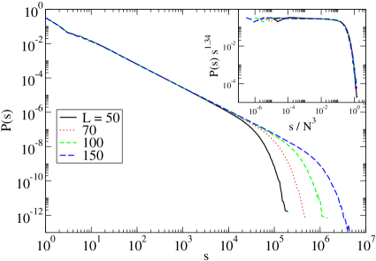
Figure 1: Log-log plot of the probability distributions of avalanche sizes for model I, for various $L$’s and for $p_{move}=10^{-1}$. Inset: data collapse of distributions rescaled according to (5).

First in Fig. 1 we show the size distributions for $p_{move}=10^{-1}$ and several $L$’s, $P_{L}(s)$. These distributions are power-laws cutoff at a size $\sim L^{\nu}$ with $\nu=3$, and the good data collapse in the inset of Fig. 1 shows that an exponent $\gamma\simeq 1.34$ can be used to describe the size distribution with a scaling form

$$P_{L}(s)\sim s^{-\gamma}F(s/L^{\nu})$$ (5)

that is typical of SOC systems. In particular, one extrapolates a diverging power-law range for $L\to\infty$.

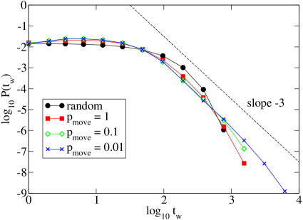
Figure 2: Log-log plot of the probability distributions of waiting times for model I with $L=100$, threshold $s_{min}=3000$, and for several $p_{move}$. Square symbols refer to the same distribution for the model with feeding randomly distributed in space. The straight dashed line represents a power-law $\sim t_{w}^{-3}$.

In Fig. 2 we show the distributions of waiting times, $P(t_{w})$, between event with size larger than $s_{min}=3000$, for a lattice with side $L=100$, and three values of the source moving rate $p_{move}=1$ (filled squares connected with dotted lines), $p_{move}=10^{-1}$ (empty squares connected with dotted lines), $p_{move}=10^{-2}$ (crosses connected with dotted lines). For comparison we also plot the distributions corresponding to random uniform feeding, which are almost exponential, as previously found boffetta1999 . The other curves instead exhibit a power-law tail that becomes wider for decreasing $p_{move}$. This behavior could be expected, as a small $p_{move}$ implies a slower diffusion of the sources and thus a higher spatial correlation between the sites were avalanches occur.

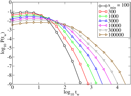
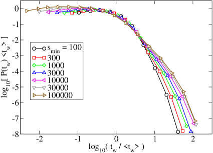
Figure 3: Log-log plot of the distributions of waiting-times for model I (with $L=150$ and $p_{move}=10^{-1}$) for different values of the threshold $s_{min}$.

Figure 4: As in Fig. 4 for the distributions rescaled by the mean waiting time.

In Fig. 4 we see the same distribution functions corresponding to a fixed value of the source moving rate $p_{move}=10^{-1}$ and different thresholds. The simulations are done for the lattice with size $L=150$. The absolute value of the exponent of the power-law decreases with the growth of the threshold $s_{min}$. Power-laws with negative exponents that are smaller in absolute value of course decay slower. Thus, in this model, correlations between events detected by using larger thresholds are qualitatively different from the ones between small events, as they have a slower decay with the waiting time.

Fig. 4 shows the same distributions rescaled by the mean waiting time. It is evident that the distribution curves do not collapse into the power-law with a given exponent, thus representing the fact that the exponent values depend on the thresholds.

These results have a twofold meaning: they again show that correlated avalanches can be found in SOC models. On the other hand, the recent results on the data collapse of the waiting time distributions of flares flares cannot be reproduced, which means that the model is missing some important feature. This should not be surprising, as our model is an extremely oversimplified system. It is also fair to say that the analysis of the results via rescaling of the waiting time distributions is a test that has not yet been used to analyze data from models outside the SOC domain.

III.2 Model II

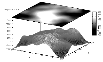
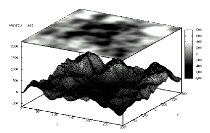
Figure 5: Two configurations of model II (with $p_{move}=10^{-2}$), one for $L=100$ and one for $L=300$.

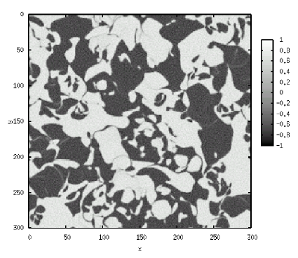
Figure 6: Field $h$ (top panel) and curvature $\Delta h$ (bottom panel) of a configuration for model II (with $L=300$ and $p_{move}=10^{-2}$).

Model II has two sources of opposite polarities that execute a random walk as the result of an idealized complex convective motion of an underlying turbulent atmosphere. While model I displays the usual profiles of the field $h$ (not shown), with a maximum at the center of the lattice, we can observe far more complex configurations in model II. Two typical configurations of the system, one for $L=100$ and one for $L=300$ (both with $p_{move}=10^{-2}$), are shown in Fig. 5. One can see that a non-trivial field landscape arises because of the complex interplay between the relaxation dynamics and the diffusion of the two sources of perturbation. In Fig. 6 one can appreciate that there is also a non-trivial relation between the field $h$ (top panel) and its corresponding curvature field $\Delta h$ (bottom panel).

It is possible that the system dynamics generates a length scale corresponding e.g. to the average distance between local minima and local maxima: the comparison between the two configurations in Fig 5, $L=100$ and $L=300$, in this case seems to confirm this hypothesis, as the typical size of the white and black areas in both “magnetograms” are similar. This length scale contrasts with the scale-free nature of SOC, as the lattice size $L$ does.

A new length scale in the model, in addition to the lattice size, could prevent the model from becoming asymptotically critical for $L\to\infty$. This scenario is supported quantitatively by Fig. 7, in which the distribution of avalanche sizes, while displaying the usual power-law range of SOC models, is cutoff at a size that essentially does not scale with $L$. While for practical purposes this is not a problem (we have a distribution with a power-law range that occupies some decades, like experimental ones), the mathematical assessment of criticality in SOC models would require also this additional length scale to diverge. This might be achieved by letting $p_{move}\to 0$, as suggested by figure 8, in which we see that the size distribution develops a wider power-law range for decreasing $p_{move}$. (Similar results are found in several SOC models when some dissipation is introduced. In our model the mobility of the sources might play a role similar to the rate of dissipation during a toppling in e.g. the Abelian sandpile.) Unfortunately, the simulation of systems with a low $p_{move}$ is much more time-consuming. Indeed, it becomes difficult to achieve a correct sampling, because it takes a too long time for the drivers to span a significant fraction of the lattice sites. Thus, we cannot assess any precise statement concerning this limit.

Model II shows distribution of waiting times with the features that we also found in model I, see figure 9. In particular, the power-law tails of the distributions have different exponents and hence the curves would not collapse upon rescaling of the times.

IV conclusions

The magnetized atmosphere of the Sun is represented in our model as a magnetic ”canopy”. The magnetic field ideally is entering perpendicular to a two-dimensional domain, with sources of perturbation undergoing a diffusion and producing local instabilities whenever the curvature of the magnetic field is too high. These instabilities are flattened out in a dynamics producing avalanches of energy release that we interpret as flares.

In a first model, we have performed numerical simulations with perturbation and boundary conditions typical of the LH-model, and we have measured the size of the avalanches and the time between avalanches of a size bigger than a given threshold. The analysis has shown that the diffusive character of the feeding sources is related to the power-law tail in the waiting time distributions between avalanches. The power-law exponents of these tails depend on the value of the diffusion rate $p_{move}$ and on the thresholds in the size of the avalanches. Thus, they are non-universal and the avalanche time series at a give scale is quantitatively and also qualitatively different from the same time series at another scale, at variance with real time series flares .

With two sources pumping perturbations of opposite polarities we obtain a second model with novel features, like typical configurations with a complex field landscape (magnetograms), and with patches of positive and negative curvature that are non-trivially related to the corresponding magnetic field. When the sources move slow enough, also this system reaches a critical regime with power-law distributions for the avalanche sizes and waiting times. This behavior is achieved even without a mechanism of magnetic reconnection, and without open boundary conditions. A length scale independent of the system size but depending on the source diffusion rate is present in this case, which prevents the system from approaching a pure SOC state for larger and larger lattices.

In order to develop a more detailed model, which could be used for a direct comparison with the observations, one should add more and different types of mechanism of energy release, for example, like the ones introduced in hughes2003 ; paczushug . It would ultimately amount to a systematic study of the processes of transformation and redistribution of the magnetic energy. The results here already reveal that temporal correlations in the energy accumulation and in the release processes can be expected from a SOC model, realizing and incorporating the clustering in space and time of the active areas of the system.

Acknowledgments
Work of B.M.S. have been supported by short term post doctoral grant at the Instituut voor Theoretische Fysica (ITF), K.U.Leuven, Grant of K.U.Leuven -PDM/06/116 and Grant of Georgian National Science Foundation - GNSF/ST06/4-098. M.B. thanks the ITF for the warm hospitality.

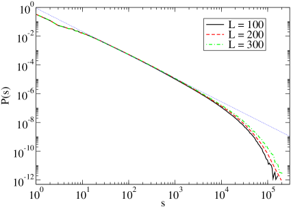
Figure 7: Log-log plot of the distributions of avalanche sizes for model II (with $p_{move}=10^{-2}$) for lattice sizes $L=100$, $200$, and $300$. The straight line interpolates the power-law range of the curves.

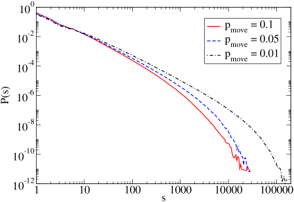
Figure 8: Log-log plot of the distributions of avalanche sizes for model II, for $L=100$ and several $p_{move}$.

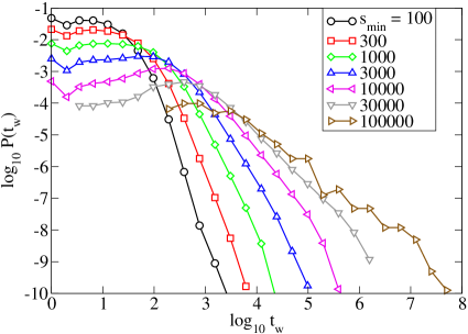
Figure 9: Log-log plot of the distributions of waiting times for model II (with $p_{move}=10^{-2}$ and $L=200$) for several thresholds.

References

- [1] P. Bak, C. Tang, K. Wiesenfeld, Phys. Rev. Lett. 59 (1987) 381.
- [2] P. Bak, How Nature works: The Science of Self-Organized Criticality, Copernicus, New York, 1996.
- [3] D. Sornette, Critical Phenomena in Natural Sciences Springer, Heidelberg, 2000.
- [4] H.J. Jensen, In Self-Organized Criticality, Cambridge University Press, 1998.
- [5] M.J. Aschwanden, T.D. Tarbell, R.W. Nightingale, C.J. Schrijver, A. Title, ApJ 535 (2000) 1047
- [6] M.J. Aschwanden, R.W. Nightingale, T.D. Tarbell, C.J. Wolfson, ApJ 535 (2000) 1027.
- [7] J. Heyvaerts, Coronal Heating Mechanisms, ed. P. Murdin, Bristol: Institute of Physics Publishing 2001.
- [8] B.M. Shergelashvili, S. Poedts, A.D. Pataraya, ApJ 642 (2006) L73.
- [9] B.M. Shergelashvili, S. Poedts, A.D. Pataraya, Proceedings of the 11th European Solar Physics Meeting ”The Dynamic Sun: Challenges for Theory and Observations”, (ESA SP-600), p.98 2005.
- [10] E.T. Lu, R.J. Hamilton, ApJ 380 (1991) L89
- [11] E.T. Lu, R.J. Hamilton, J.M. McTiernan, K.R. Bromund, ApJ 412 (1993) 841.
- [12] E.N. Parker, Sol. Phys. 121 (1989) 271.
- [13] P.A. Sturrock, P. Kaufman, R.L. Moore and D.F. Smith Sol. Phys. 94 (1984) 341.
- [14] P.A. Sturrock, W.W. Dixon, J.A. Klimchuk, S.K. Antiochos, ApJ 356 (1990) L31.
- [15] E.N. Parker, ApJ 330 (1988) 474.
- [16] H. Isliker, A. Anastasiadis, L. Vhalos, A&A 363 (2000) 1134.
- [17] L. Vlahos, H. Isliker, F. Lepreti, ApJ 608 (2004) 540.
- [18] V. Krasnoselskikh, O. Podladchikova, B. Lefebvre, N. Vilmer A&A 382 (2002) 699.
- [19] O. Podladchikova, T. Dudok de Wit, V. Krasnoselskikh, B. Lefebvre, A&A 382 (2002) 713.
- [20] G. Boffetta, V. Carbone, P. Giuliani, P. Veltri, A. Vulpiani, Phys. Rev. Lett. 83 (1999) 4662.
- [21] M. Baiesi, C. Maes, Europhys. Lett. 75 (2006) 413.
- [22] R. Woodard, D.E. Newman, R. Sánchez, B.A. Carreras, Physica A 373 (2007) 215.
- [23] M. De Menech, A.L. Stella, Physica A 309 (2002) 289.
- [24] There are other mechanisms for producing a nontrivial (critical) temporal statistics (see [22, 21, 23] and references therein. For example, one can also confine the random driving to the boundary of the domain, see: H.J. Jensen, Phys. Rev. Lett. 64 (1990) 3103.
- [25] Á. Corral, Phys. Rev. E 68 (2003) 035102.
- [26] P. Bak, K. Christensen, L. Danon, T. Scanlon, Phys. Rev. Lett. 88 (2002) 178501.
- [27] M. Baiesi, M. Paczuski, A.L. Stella, Phys. Rev. Lett. 96 (2006) 051103.
- [28] M. Paczuski, S. Boettcher, M. Baiesi, Phys. Rev. Lett. 95 (2005) 181102.
- [29] D. Hughes, M. Paczuski, R.O. Dendy, P. Helander, K.G. McClements, Phys. Rev. Lett. 90 (2003) 131101-1.
- [30] M. Paczuski, D. Hughes, Physica A. 342 (2004) 158.