Nodal points and the transition from ordered to chaotic Bohmian trajectories

Abstract

We explore the transition from order to chaos for the Bohmian trajectories of a simple quantum system corresponding to the superposition of three stationary states in a 2D harmonic well with incommensurable frequencies. We study in particular the role of nodal points in the transition to chaos. Our main findings are: a) A proof of the existence of bounded domains in configuration space which are devoid of nodal points, b) An analytical construction of formal series representing regular orbits in the central domain as well as a numerical investigation of its limits of applicability. c) A detailed exploration of the phase-space structure near the nodal point. In this exploration we use an adiabatic approximation and we draw the flow chart in a moving frame of reference centered at the nodal point. We demonstrate the existence of a saddle point (called X-point) in the vicinity of the nodal point which plays a key role in the manifestation of exponential sensitivity of the orbits. One of the invariant manifolds of the X-point continues as a spiral terminating at the nodal point. We find cases of Hopf bifurcation at the nodal point and explore the associated phase space structure of the nodal point - X-point complex. We finally demonstrate the mechanism by which this complex generates chaos. Numerical examples of this mechanism are given for particular chaotic orbits, and a comparison is made with previous related works in the literature.

1 Introduction

The formulation of quantum mechanics based on Bohm’s trajectories (de Broglie 1926, Bohm 1952a,b) has attracted considerable interest in recent years because it offers a powerful tool to visualize quantum processes in terms of quantum orbits. According to the Bohmian interpretation (see Bohm and Hiley 1993 and Holland 1993 for reviews) the particles are guided by the Schrödinger field via deterministic equations of motion. In this approach the moving particles, together with the Schrödinger field, form the basic ingredients of objective realilty at the quantum level. On the other hand, in orthodox quantum mechanics the orbits do not refer to deterministic particles’ motions, but they represent the streamlines of the probability current ${\mathbf{j}}=(\psi^{*}\nabla\psi-\psi\nabla\psi^{*})/2i$ (we set $\hbar=1$). Thus they represent a ‘Lagrangian’ (Holland 2005) or ‘hydrodynamical’ (Madelung 1926) description of the quantum probability flow, while the Schrödinger equation yields the Eulerian description of the same flow. At any rate, the descriptive power of the Bohmian approach is independent of its ontological interpretation. In fact, applications of Bohm’s trajectories in the literature have so far successfully addressed such basic quantum processes as the two-slit experiment (Phillipidis 1979), the spin measurement via Stern-Gerlach devices (Dewdney et al. 1986), tunneling through potential barriers (Hirschfelder et al. 1974, Skodje et al. 1989, Lopreore and Wyatt 1999), ballistic electron transport (Beenakker and van Houten 1991), superfluidity (Feynman Lectures, Feynman et al. 1963), etc. (see Wyatt 2005 for a review of applications of quantum dynamics with trajectories).

In the present paper we focus on one particular aspect of Bohm’s theory that refers to the distinction of the Bohmian trajectories into regular and chaotic. A number of studies in the literature (e.g. Dürr et al. 1992, Faisal and Schwengelbeck 1995, Parmenter and Valentine 1995, de Polavieja 1996, Dewdney and Malik 1996, Iacomelli and Pettini 1996, Frisk 1997, Konkel and Makowski 1998, Wu and Sprung 1999, Makowski et al. 2000, Cushing 2000, Falsaperla and Fonte 2003, de Sales and Florencio 2003, Wisniacki and Pujals 2005, Valentini and Westman 2005, Efthymiopoulos and Contopoulos 2006) have so far converged to the conclusion that generic quantum systems of more than one degrees of freedom are characterized by the coexistence, in the configuration space, of both regular and chaotic orbits. Some established results regarding this distinction are:

a) The regular or chaotic character of the quantum mechanical orbits does not necessarily correlate with the character of the classical orbits of the same system, i.e., there are examples of systems with classically regular and quantum mechanically chaotic orbits, or vice versa (see Efthymiopoulos and Contopoulos 2006 for a review).

b) The emergence of chaos is associated with the existence of ‘nodal points’ in the configuration space, i.e., points of the configuration space at which the Schrödinger field becomes null. In some particular examples it has been possible to identify a mechanism by which the approach of an orbit near a nodal point introduces chaos (Makowski et al. 2000, Wisniaski and Pujals 2005). However the general problem of the mechanism of transition from order to chaos for the Bohmian orbits is still largely unexplored.

c) In some cases it has been shown that the extent of chaos is related to the number and spatial distribution of the nodal points in the configuration space (Frisk 1997, Wisniacki et al. 2006). However, in other cases we find the manifestation of strong chaos even if only one nodal point is present. This problem is important because it has been shown that, when the degree of chaos is large, it is possible to obtain an asymptotic convergence of the distribution $p$ of an ensemble of Bohmian trajectories to Born’s rule $p=|\psi|^{2}$, via a Bohm-Vigier (1954) stochastic mechanism (Valentini and Westman 2005, Efthymiopoulos and Contopoulos 2006), without having to postulate this rule.

Our purpose in the present paper is to study how the transition from regular to chaotic motion takes place by considering the orbits of a very simple quantum system, namely the superposition of three eigenstates in a Hamiltonian system of two independent harmonic oscillators. Parmenter and Valentine (1995,1996) demonstrated that when the two oscillator frequencies are incommensurable, the configuration space is filled by both regular and chaotic orbits (the initial claim that all the orbits were chaotic (Parmenter and Valentine 1995) was corrected by Parmenter and Valentine (1996), and by Efthymiopoulos and Contopoulos (2006)). The same coexistence was found by Wisniacki and Pujals (2005) when the frequencies are commensurable but the ampitudes of the superposed eigenfunctions have a complex ratio, and by Konkel and Makowski (1998) in the case of a particle in a box with infinite walls. In the above cases there is only one nodal point which influences the orbits and introduces chaos. Our aim below is, then, to study the transition from order to chaos from two different points of view: a) topologically, i.e. we seek to distinguigh which domains of initial conditions lead to regular or chaotic motion and what theoretical criteria can be devised in order to separate these domains, and b) dynamically, i.e., we seek to identify the dynamical mechanism behind the transition from order to chaos.

The following is an outline of the paper and of the main results:

a) Section 2 contains a proof of the existence of domains in configuration space where nodal points cannot appear. In our considered example the size of these domains depends on the relative amplitudes of the three eigenfunctions and specific quantitative estimates of this dependence are given, which are compared to numerical results.

b) In their domain of analyticity (i.e. far from nodal points), the equations of motion admit solutions expandable in series of a properly defined small parameter (section 3). The series’ terms can be determined by an iterative algorithm. The resulting solutions define theoretical orbits which are, by definition, regular. The theoretical orbits explain all the basic characteristics of the regular orbits as found by numerical integration. In particular they explain the frequencies, the form, the limits and the inner deflections of regular orbits.

c) Section 4 passes to the other limit, of motion, close to the nodal points. In order to unravel the mechanism by which the orbits approaching the nodal point become chaotic, the key point is to take into account the motion of the nodal point itself by passing to a description of the orbits in a moving frame of reference centered at the (moving) nodal point. The main characteristics of the orbits in this frame are found by expansions of the equations of motion in terms of a new small parameter, i.e., the distance $R=\epsilon$ from the nodal point. The angular frequency of motion near the nodal point is of order $O(1/\epsilon^{2})$, a fact allowing us to use an adiabatic approximation. In this approximation, the flow lines near the nodal point are spirals terminating at the nodal point. However, the flow further away from the nodal point is quite complicated and it is studied in detail. In particular, we demonstrate how this flow is related to the manifestation of chaos in the system. The main results are derived theoretically and then substantiated by detailed numerical experiments.

d) Finally, we discuss (section 5) how do our results compare with previous works in the literature on nodal points, and we end with the conclusions (section 6).

2 Limits of nodal lines

We study the quantum orbits in the Hamiltonian model of two uncoupled oscillators:

$$H={1\over 2}(p_{x}^{2}+p_{y}^{2})+{1\over 2}(x^{2}+(cy)^{2})$$ (1)

when the guiding field is the superposition of three stationary states (Parmenter and Valentine 1995):

$$\psi(x,y,t)=e^{-{x^{2}+cy^{2}\over 2}-i{(1+c)t\over 2}}\big{(}1+axe^{-it}+bc^{1/2}xye^{-i(1+c)t}\big{)}~{}~{}.$$ (2)

The equations of motion (de Broglie 1926, Bohm 1952a) are

$$(\dot{x},\dot{y})\equiv\Im\bigg{(}{\vec{\nabla}\psi\over\psi}\bigg{)}$$ (3)

where $\Im$ denotes the imaginary part of each of the components of the vector $\vec{\nabla}\psi/\psi$, or

$${dx\over dt} = -{a\sin t+bc^{1/2}y\sin(1+c)t\over G}$$ (4)

$${dy\over dt} = -{bc^{1/2}x\big{(}ax\sin ct+\sin(1+c)t\big{)}\over G}$$

with

$$G=1+2ax\cos t+2bc^{1/2}xy\cos(1+c)t+a^{2}x^{2}+2abc^{1/2}x^{2}y\cos ct+b^{2}cx^{2}y^{2}~{}~{}.$$ (5)

The equations of motion (4) become singular whenever $G=0$. From (5) we then find the equations of the nodal points:

$$x_{0}=-{\sin(1+c)t\over a\sin ct},~{}~{}~{}~{}y_{0}=-{a\sin t\over bc^{1/2}\sin(1+c)t}~{}~{}.$$ (6)

When the frequency $c$ is a rational number, the nodal points describe periodic motions in the configuration space $(x,y)$, along a finite number of nodal lines (Figure 1a). However, when $c$ is irrational there is an infinite number of nodal lines that fill open domains of the space $(x,y)$ (Figure 1b). As shown in section 3, a theoretical approximation of the regular orbits can be obtained in the complement of the domain of nodal lines. We thus first provide, in this section, rigorous bounds for the domain of nodal lines. In particular, we prove the following proposition: when the relative amplitudes $a,b$ are non-zero, the domain of nodal lines is bounded by a set of limiting hyperbolae.

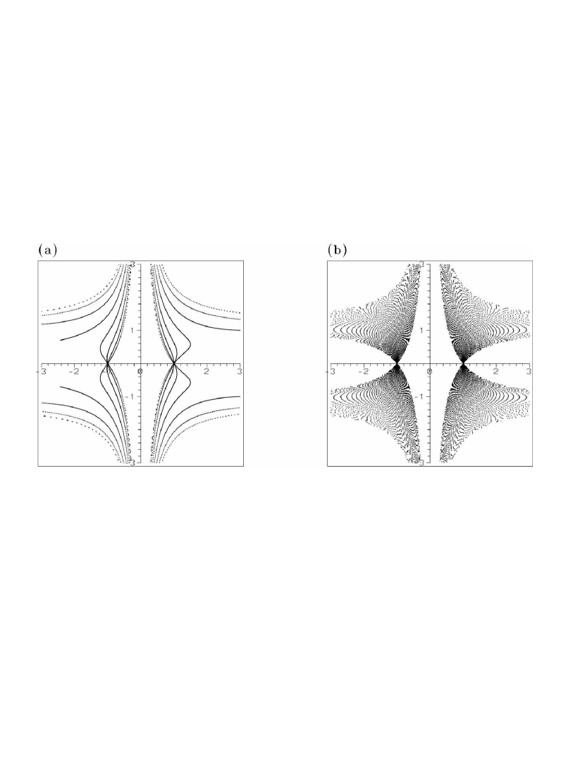
Figure 1: Nodal lines given by Eqs.(6) for $a=1$, $b=1$, $0\leq t\leq 1000$ and (a) $c=7/10$, (b) $c=\sqrt{2}/2$.

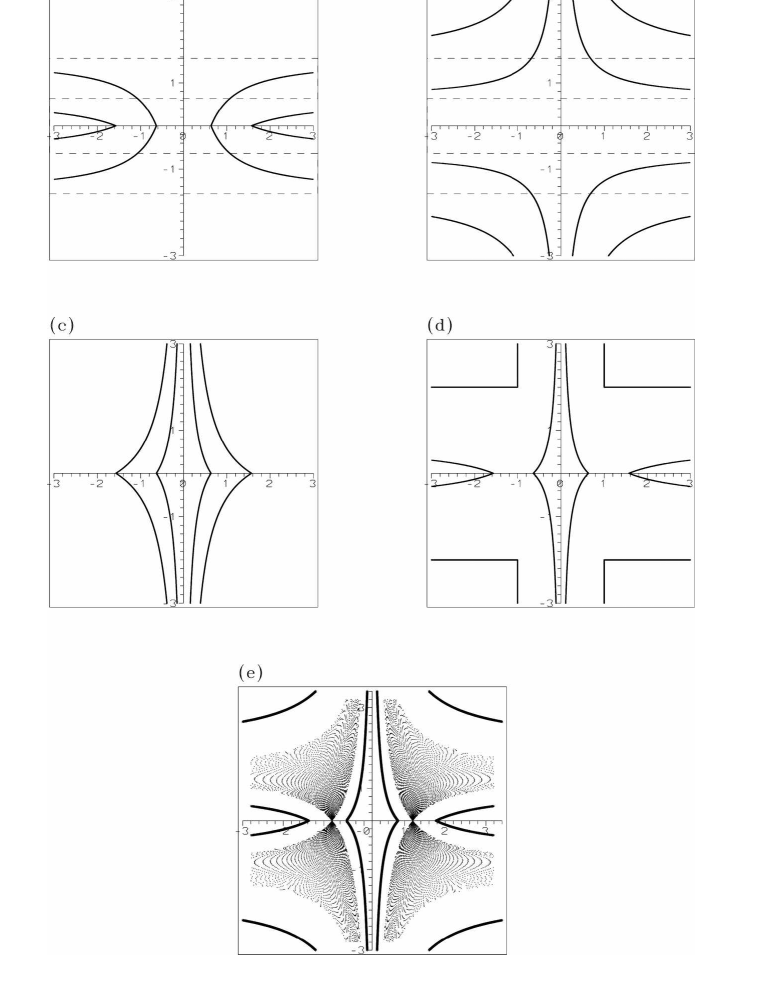
Figure 2: The limits of nodal lines as determined by (a) Eq.(12), (b) Eq.(13), (c) Eq.(14), (d) Eqs.(15) and (16). (e) The nodal lines given by Eq.(6) for $a=1$, $b=1$, $c=\sqrt{2}/2$, $0\leq t\leq 1000$, superposed to the less restrictive of all the limits shown in panels (a) to (d).

To this end, we write $x_{0}=-X_{0}/a$ and $y_{0}=-aY_{0}/bc^{1/2}$, where

$$X_{0}={\sin(1+c)t\over\sin ct},~{}~{}~{}~{}Y_{0}={\sin t\over\sin(1+c)t}~{}~{}.$$ (7)

We make use of the following lemma:

(i) $$\forall~{}u\in{\cal R}~{}\mbox{with}~{}0\leq u\leq\pi/2,~{}~{}\exists~{}\delta>0~{}\mbox{with}~{}{2\over\pi}\leq\delta\leq 1:~{}\sin u=\delta u$$ (8)

(ii) $$\forall~{}u\in{\cal R}~{}\mbox{with}~{}0\leq u\leq\pi,~{}~{}\sin u\leq u~{}~{}.$$

In order to find the bounds of $(|X_{0}|,|Y_{0}|)$ we consider all the $4\times 4=16$ possible combinations of the trigonometric arguments $t,(1+c)t$ being in any of the four quartiles of the trigonometric circle, i.e.,

$$(1+c)t = 2k_{1}\pi\pm t_{1},~{}\mbox{or}~{}(1+c)t=(2k_{1}+1)\pi\pm t_{1}$$

$$t = 2k_{2}\pi\pm t_{2},~{}\mbox{or}~{}t=(2k_{2}+1)\pi\pm t_{2}$$ (9)

with $(k_{1},k_{2})\in{\cal Z}^{2}$ and $0\leq t_{1}\leq\pi/2$, $0\leq t_{2}\leq\pi/2$. Taking now $ct=(1+c)t-t$ we find the following possibilities for $|\sin(ct)|$:

$$|\sin(ct)|=|\sin(t_{1}\pm t_{2})|~{}~{}.$$ (10)

We then distinguish four cases, namely cases A,B with $|\sin ct|=|\sin(t_{1}-t_{2})|$, and cases C,D with $|\sin ct|=|\sin(t_{1}+t_{2})|$.

Case A: $t_{1}>t_{2}$ (and $|\sin(ct)|=\sin(t_{1}-t_{2})$). Since $t_{1}-t_{2}\leq\pi/2$, according to the Lemma (8)(i)

$$\exists~{}\delta_{i}>0,~{}i=1,2,3:~{}{2\over\pi}\leq\delta_{i}\leq 1~{}\mbox{such that}~{}$$

$$|\sin(1+c)t|=\delta_{1}t_{1},|\sin t|=\delta_{2}t_{2},~{}|\sin ct|=\sin(t_{1}-t_{2})=\delta_{3}(t_{1}-t_{2})$$

or

$$|X_{0}|={\delta_{1}t_{1}\over\delta_{3}(t_{1}-t_{2})},~{}~{}|Y_{0}|={\delta_{2}t_{2}\over\delta_{1}t_{1}}~{}~{}.$$ (11)

From (11) then follows the inequality:

$${1\over{\pi\over 2}-|Y_{0}|}\leq|X_{0}|\leq{1\over{2\over\pi}-|Y_{0}|}$$ (12)

which is shown graphically in Fig.2a. When $|Y_{0}|=0$, $|X_{0}|$ is between $2/\pi$ and $\pi/2$.

Case B: $t_{2}>t_{1}$ (and $|\sin(ct)|=\sin(t_{2}-t_{1})$). Working in the same way as for Case A we find the inequality

$${1\over{\pi\over 2}|Y_{0}|-1}\leq|X_{0}|\leq{1\over{2\over\pi}|Y_{0}|-1}$$ (13)

shown graphically in Fig.2b. When $|X_{0}|\rightarrow\infty$, $|Y_{0}|$ is between $2/\pi$ and $\pi/2$ (dashed asymptotic curves in Fig.2b).

Case C: $t_{1}+t_{2}\leq\pi/2$ (and $|\sin(ct)|=\sin(t_{1}+t_{2})$). In this case we find that

$$\exists~{}\delta_{i}>0,~{}i=1,2,3:~{}{2\over\pi}\leq\delta_{i}\leq 1~{}\mbox{such that}~{}$$

$$|\sin(1+c)t|=\delta_{1}t_{1},|\sin t|=\delta_{2}t_{2},~{}|\sin ct|=\sin(t_{1}+t_{2})=\delta_{3}(t_{1}+t_{2})$$

or

$${2\over\pi(|Y_{0}|+1)}\leq|X_{0}|\leq{\pi\over 2(|Y_{0}|+1)}$$ (14)

(Fig.2c). When $|Y_{0}|=0$, $|X_{0}|$ is between $2/\pi$ and $\pi/2$.

Case D: $t_{1}+t_{2}>\pi/2$ (and $|\sin(ct)|=\sin(t_{1}+t_{2})$). In this case

$$\exists~{}\delta_{i}>0,~{}i=1,2,3:~{}{2\over\pi}\leq\delta_{i}\leq 1~{}\mbox{such that}~{}$$

$$|\sin(1+c)t|=\delta_{1}t_{1},|\sin t|=\delta_{2}t_{2},~{}|\sin ct|=\sin(t_{1}+t_{2})=\sin(\pi-(t_{1}+t_{2}))=\delta_{3}(\pi-t_{1}-t_{2})$$

implying

$${2\over\pi({\pi\over 2}|Y_{0}|+1)}\leq|X_{0}|\leq{1\over{2\over\pi}-|Y_{0}|}~{}~{}.$$ (15)

Furthermore, if $t_{1}\leq\pi/4$ (case D₁) we have $t_{2}\geq\pi/4$ and $\pi-(t_{1}+t_{2})\geq\pi/4$. The Eqs.(7) and (2) imply that $|X_{0}|\leq 1$ and $|Y_{0}|\geq 1$. On the other hand, if $t_{1}>\pi/4$ (case D₂) we have

$$|Y_{0}|={\sin t\over\delta_{1}t_{1}}<{1\over\delta_{1}{\pi\over 4}}<2~{}~{}.$$

The union of the two possibilities yields:

$$|X_{0}|\leq 1~{}~{}~{}\mbox{or}~{}~{}~{}|Y_{0}|\leq 2~{}~{}.$$ (16)

The inequalities (15) and (16) are shown graphically in Fig. (2d). When $|Y_{0}|=0$, $|X_{0}|$ is between $2/\pi$ and $\pi/2$.

The less restrictive of all bounds determine the permissible domain for nodal points. The outer limit (13) of Case B is less restrictive than the limit $|X_{0}|$ of Case D if $1/({2\over\pi}|Y_{0}|-1)<1$, i.e. if $|Y_{0}|<\pi$ (in the exceptional case that $|Y_{0}|>\pi$ the limit $|X_{0}|=1$ is less restrictive than the limit of case B). Figure 2e shows the analytical estimates for the bounds of the nodal lines compared to the numerical determination of the nodal lines in the variables $(x_{0},y_{0})$ for the parameters $a=b=1$, $c=\sqrt{2}/2$. The further restrictions of the cases A-D are also satisfied if $t_{1}$ and $t_{2}$ take the values specified in these particular cases. The main conclusion is that there is a central domain, with boundary defined by the innermost arcs of limiting hyperbolae, that is never crossed by nodal points. There is also an outer domain, at large distances from the center, which is again prohibited to nodal points. By calculating many orbits, our numerical evidence is that the orbits lying within these domains are regular. In particular, we now turn our attention to the analytical determination of the regular orbits for the central domain free of nodal points.

3 Integrals of motion and the bounds of regular orbits

According to the analysis of the previous section, a lower bound for the distance of a nodal point $(x_{0},y_{0})$ from the origin $(0,0)$ is given by $d_{min}=(x_{0,min}^{2}+y_{0,min}^{2})^{1/2}$, with $(x_{0}=X_{0,min}/a,y_{0}=aY_{0,min}/bc^{1/2})$, and $X_{0,min},Y_{0,min}$ corresponding to the closest approach of the innermost limiting hyperbola (Eq.(15)) to the origin, i.e.

$${\pi^{4}X_{0,min}^{4}\over 16}+{\pi X_{0,min}\over 2}-1=0,~{}~{}Y_{0,min}={2\over\pi}\Bigg{(}{2\over\pi X_{0,min}}-1\Bigg{)}$$

or $X_{0,min}=0.461226$, $Y_{0,min}=0.242092$. When $a$ and $b$ are large, the distance $d_{min}$ is small and the inner domain free of nodal points is small. On the other hand, in the limit $a\rightarrow 0$, $b\rightarrow 0$ we have $d_{min}\rightarrow\infty$ and the whole space is free of nodal points. This implies that if we look for analytic solutions of the equations of motion (4), i.e., free of singularities in the neighborhood of the origin, we may consider $a,b$ in Eq.(5) as small parameters, and expand $1/G$ in Eq.(4) in a power series of these parameters. This results in solutions

$$x(t)=x_{0}+x_{1}(t)+x_{2}(t)+...,~{}~{}~{}y(t)=y_{0}+y_{1}(t)+y_{2}(t)+...,~{}~{}~{}$$ (17)

where the functions $x_{n}(t)$, $y_{n}(t)$ are of order $n$ in the amplitudes $a$ or $b$. The convergence of these series, which are of the form of the ‘third integral’ (Contopoulos 1960), is an open problem. However, our numerical evidence below is that the form of theoretical orbits derived by these series fits well the form of the numerical orbits for small parameters $a,b$.

In the zeroth order approximation all the solutions are equilibria $x(t)=x_{0}$, $y(t)=y_{0}$. This corresponds to the limit $a=b=0$, in which the guiding $\psi-$field is a bound stationary state, and all the quantum orbits are neutral equilibria. On the other hand, when higher order terms are taken into account, Eqs.(17) can be inverted, and, provided that the series converge, they yield the integrals of motion

$$x-x_{1}(t)-x_{2}(t)-...=x_{0},~{}~{}~{}y-y_{1}(t)-y_{2}(t)-...=y_{0}$$ (18)

implying that the resulting orbits are, by definition, regular.

The solutions (17) are found recursively, i.e., order by order, giving $x_{k},y_{k}$ as explicit trigonometric expressions in $t$, with two basic frequencies $\nu_{1}=1$ and $\nu_{2}=c$.

The first order equations read

$${dx_{1}\over dt}=-a\sin t-{bc^{1/2}}y_{0}\sin((1+c)t),~{}~{}~{}{dy_{1}\over dt}=-bc^{1/2}x_{0}\sin((1+c)t)$$ (19)

and they can be readily integrated yielding

$$x_{1}(t) = A_{1}+a\cos t+bc^{1/2}y_{0}{\cos((1+c)t)\over 1+c}$$

$$y_{1}(t) = B_{1}+bc^{1/2}x_{0}{\cos((1+c)t)\over 1+c}$$ (20)

where $A_{1},B_{1}$ are integration constants. Since we wish to absorb the whole dependence of the solution on the initial conditions in the $x_{0},y_{0}$ part of the solution, we select the values of $A_{1},B_{1}$ such that $x_{1}(0)=y_{1}(0)=0$.

In a similar way we treat the second order equations, finding the solutions

$$x_{2}(t) = -{a^{2}x_{0}\over 2}\cos(2t)-{b^{2}cx_{0}\over(1+c)^{2}}\cos((1+c)t)$$

$$- {b^{2}cx_{0}\over 2(1+c)}\bigg{(}y_{0}^{2}-{1\over 2(1+c)}\bigg{)}\cos(2(1+c)t)$$

$$- {2abc^{1/2}x_{0}y_{0}\over 2+c}\cos((2+c)t)+A_{2}$$

and

$$y_{2}(t) = -\bigg{(}{abc^{1/2}\over 1+c}+{b^{2}cy_{0}\over(1+c)^{2}}\bigg{)}\cos((1+c)t)$$

$$- {b^{2}cy_{0}\over 2(1+c)}\bigg{(}x_{0}^{2}-{1\over 2(1+c)}\bigg{)}\cos(2(1+c)t)$$

$$+ {ab\over 2c^{1/2}}\cos(ct)-{abc^{1/2}\over 2+c}\bigg{(}x_{0}^{2}-{1\over 2}\bigg{)}\cos((2+c)t)+B_{2}$$

respectively. The integration constants $A_{2},B_{2}$ are also given values such that $x_{2}(0)=y_{2}(0)=0$.

We can prove the consistency of the above construction, i.e., that no secular terms can appear in the above recursive scheme. The proof follows by induction: If the solutions $x_{i}(t),y_{i}(t)$, $i=1,...,n$ contain only cosine terms (of the form $\cos((m_{1}+m_{2}c)t)$ with $m_{1},m_{2}$ integer, then, the expansion

$${1\over G}=1+\sum_{k=1}^{n}(-1)^{k}\Bigg{[}2ax^{(n)}\cos t+2bc^{1/2}x^{(n)}y^{(n)}\cos(1+c)t$$

$$+a^{2}(x^{(n)})^{2}+2abc^{1/2}(x^{(n)})^{2}y^{(n)}\cos ct+b^{2}c(x^{(n)})^{2}(y^{(n)})^{2}\Bigg{]}^{k}+\ldots$$

with

$$x^{(n)}(t)=x_{0}(t)+x_{1}(t)+\ldots+x_{n}(t),~{}~{}y^{(n)}(t)=y_{0}(t)+y_{1}(t)+\ldots+y_{n}(t)$$

contains only powers of cosine terms, yielding again only cosine terms since $\cos w_{1}\cos w_{2}=$ $(\cos(w_{1}+w_{2})+\cos(w_{1}-w_{2}))/2$. Thus, the equations of motion in order $n+1$ yield only sine terms, since $1/G$ in Eqs.(4) is multiplied only by sine terms and $\sin w_{1}\cos w_{2}=$ $(\sin(w_{1}+w_{2})+\sin(w_{1}-w_{2}))/2$. If for some terms we have $w_{1}=(m_{1}+m_{2}c)t$, $w_{2}=(m_{1}^{\prime}+m_{2}^{\prime}c)t$, the sine terms produced in the equations of motion are $\sin(m_{1}+m_{1}^{\prime}+m_{2}c+m_{2}^{\prime}c)t$, or $\sin(m_{1}-m_{1}^{\prime}+m_{2}c-m_{2}^{\prime}c)t$. If ($m_{1}=\pm m_{1}^{\prime}$ and $m_{2}=\pm m_{2}^{\prime}$), or, $c$ is rational and equal to $c=-(m_{1}\pm m_{1}^{\prime})/(m_{2}\pm m_{2}^{\prime})$, one of the sine terms in the equation of motion becomes equal to zero (resonance). However, the resonances do not create any secular term in the solutions of the equations since the associated terms simply disappear from the r.h.s of Eqs.(4). Thus, the equations in the next order give $dx_{n+1}/dt$ and $dy_{n+1}/dt$ as sums of sine terms, and it follows that, if $x^{(n)}$ and $y^{(n)}$ are sums of cosine terms, $x_{n+1}$ and $y_{n+1}$ are also sums of cosine terms. Thus, no secular terms appear in the solutions $x^{(n)}$, $y^{(n)}$, $\forall n=1,\ldots\infty$ since $x^{(1)},y^{(1)}$ are sums of cosine terms.

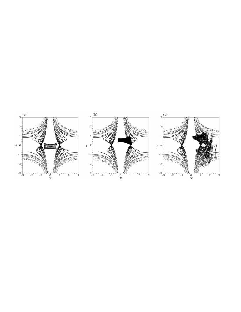
Figure 3: Three orbits in the equations of motion (4) for $a=b=1$, $c=\sqrt{2}/2$ and $0\leq t\leq 1000$. The initial conditions are (a) $x(0)=0.75$, $y(0)=0.25$ (regular, not overlapping with the domain of nodal lines), (b) $x(0)=y(0)=1$ (regular, partly overlapping with the domain of nodal lines), and (c) $x(0)=y(0)=1.4$ (chaotic).

The main characteristics of the regular orbits in the central region can be understood in terms of the above equations. In particular:

a) The regular orbits are quasi-periodic, i.e., they are given as double Fourier series with two fundamental frequencies $\nu_{1}$, $\nu_{2}$, which have constant values $\nu_{1}=1$, $\nu_{2}=c$. This fact is important because it implies that there is no dependence of the frequencies of the orbits on the amplitudes of the oscillations. This is different from what is usually encountered in the case of classical nonlinear dynamical systems, in which the frequencies depend, in general, on the amplitudes. On the contrary, the quantum mechanical orbits in this system are completely degenerate with respect to their fundamental frequencies.

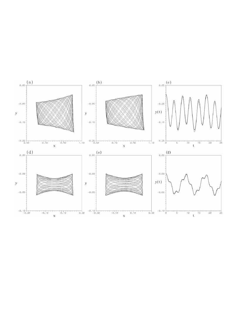
Figure 4: (a) An orbit with $a=b=0.2$, $c=\sqrt{2}/2$ and initial conditions $x(0)=1$, $y(0)=0$. (b) The theoretical approximation to the same orbit up to terms of second degree in $a$ and $b$, given by Eqs.(23) and (3). (c) The time evolution of $y(t)$ for the same orbit. The numerical and theoretical curves almost coincide. (d) Same as (a) but with initial conditions $x(0)=y(0)=0$. (e) Same as (b) but for the orbit (d). (f) Same as (c) but for the orbit (d); the secondary local maxima of $y(t)$ correspond to deflections of the orbit inside its ‘box’ limit.

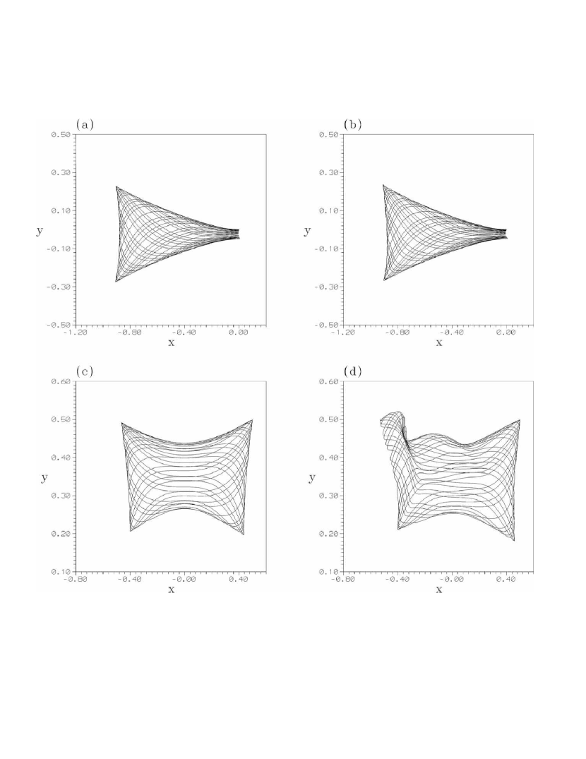
Figure 5: Numerical versus theoretical orbits for $a=b=0.5$, $c=\sqrt{2}/2$. (a) Numerical orbit with initial conditions $x(0)=y(0)=0$. (b) The theoretical approximation of orbit (a) with an expansion up to terms of 10-th degree in $a$,$b$. (c) Numerical orbit with initial conditions $x(0)=0.5$, $y(0)=0$. (d) Same as in (b) but for the orbit (c).

b) The amplitudes of all the trigonometric terms depend on $a$ and $b$, but in many terms they depend also on the initial conditions $x_{0},y_{0}$. The former condition ensures that for $a,b$ sufficiently small a regular orbit does not overlap with the domain of nodal lines. This is because the amplitudes of oscillations are $O(a)$ and $O(bc^{1/2})$ in the $x$ and $y$ axes respectively (Eqs.(3)), while the minimum distance of a nodal point from the center is of order $O(|1/a|+|1/b|)$ (section 2). Numerically we find such regular orbits for $a,b$ as high as $a=b=1$ (Figure 3a). However, the oposite is not true, namely an orbit overlaping partly with the domain of nodal lines may still be regular (Figure 3b). In fact, we find numerically that while there is a spatial overlap of the domains of the orbit and of the nodal lines, the time evolution of both the orbit and the nodal point is such that their distance is always large (of order unity). Thus when an orbit enters some region containing nodal lines the nodal point is far from this region. However, we also find numerically that if an orbit has significant overlap with the domain of nodal lines, the orbit is, in general, chaotic (Figure 3c).

c) In the lowest approximation, when $x_{0}\neq 0$ the theoretical orbits are ‘box orbits’ (Eqs.(3)) like in the classical case. However, when higher order terms are taken into account, some box orbits develop deflections internal to the box, while other box orbits have deflections only at the boxes’ limits, depending on the value of $x_{0},y_{0}$. A simple example is provided by orbits starting on the axis $y_{0}=0$. Then, the equations of the orbits are simplified considerably . We have, up to second order:

$$x(t) = x_{0}+a[\cos t-1]-{a^{2}x_{0}\over 2}[\cos 2t-1]-$$ (23)

$${b^{2}cx_{0}\over(1+c)^{2}}[\cos((1+c)t)-1]+{b^{2}cx_{0}\over 4(1+c)^{2}}[\cos(2(1+c)t)-1]$$

$$y(t) = {bcx_{0}\over 1+c^{2}}[\cos((1+{1\over c^{2}})t)-1]$$

$$- {abc^{1/2}\over 1+c}[\cos((1+c)t)-1]+{ab\over 2c^{1/2}}[\cos(ct)-1]$$

$$- {abc^{1/2}\over 2+c}(x_{0}^{2}-{1\over 2})[\cos((2+c)t)-1]~{}~{}.$$

In Eq.(23) the first order term $a[\cos t-1]$ depends only on $a$, yielding an oscillation of amplitude $2a$, while in Eq.(3), the first order term $bc^{1/2}x_{0}[\cos((1+c)t)-1]/(1+c)$ depends on both $b$ and $x_{0}$. For all initial conditions with $|x_{0}|=O(1)$, this term is dominant over the second order terms in Eq.(3). Thus the orbit is a deformed parallelogram, i.e., it resembles to classical box orbits (Figure 4a,b,c). On the other hand, if $|x_{0}|\rightarrow 0$, this term becomes small, while the second order terms, not depending on $x_{0}$, become now important. This means that secondary oscillations of the function $y(t)$ are developed, that may also yield local minima or maxima besides the main minimum or maximum defined by the first order Fourier component of (3). This causes the orbit to develop deflections in the $y-$ direction inside the box. A numerical example of this behavior is demonstrated in Figs. 4d,e,f.

Figure 5 shows some further examples of theoretical orbits calculated by the above series, via a computer program implementing the recursive algorithm up to the 10th order. As expected in any kind of perturbative series, as $a,b$ increase one needs higher order terms to obtain a good approximation of the orbits. In fact, as already analyzed, the approximation depends also on the values of the initial conditions $x_{0},y_{0}$ which appear in the amplitudes of the trigonometric terms of Eqs.(3), (3) and (3). Thus, when $x_{0}=y_{0}=0$, the theoretical orbit for $a=b=0.5$ (Fig.5a,b) fits well the numerical orbit, while if the series are truncated at orders well below 10 the agreement is not so good. On the other hand for the same amplitudes $a,b$ the fit is not good when $x_{0}=y_{0}=0.5$ (Fig.5c,d). Now, in any perturbation theory the analytical results are precise up to values of the small parameters smaller than the values for which regular orbits are found numerically. Thus, in our case we find that for amplitudes larger than $a=b=0.75$ the approximation of the numerical orbits by series yields no longer accurate results, despite the fact that we still find numerically many regular orbits.

4 The dynamics close to nodal points and the transition to chaos

4.1 Phase space structure close to nodal points and the adiabatic approximation

Having demonstrated the existence of regular orbits far from the nodal points, we now examine the motion in the other limit, i.e., close to a nodal point. Our main remark in the sequel is that the phenomena relevant to the transition to chaos are unraveled when one considers the passage of the orbits in the neighborhood of the nodal point in a moving frame of reference that is centered at the nodal point. Introducing $u=x-x_{0}$, $v=y-y_{0}$, the equations of motion in the moving frame read:

$${du\over dt} = -{bc^{1/2}v\sin(1+c)t\over G}-\dot{x}_{0}$$

$${dv\over dt} = {bc^{1/2}u\sin(1+c)t-abc^{1/2}u^{2}\sin ct\over G}-\dot{y}_{0}$$ (25)

where $G=G_{2}+G_{3}+G_{4}$ with

$$G_{2} = {u^{2}\over x_{0}^{2}}-2bc^{1/2}uv\cos(1+c)t+b^{2}cx_{0}^{2}v^{2}$$

$$G_{3} = -{2bc^{1/2}\over x_{0}}u^{2}v\cos(1+c)t+2b^{2}cx_{0}uv^{2}$$ (26)

$$G_{4} = b^{2}cu^{2}v^{2}$$

and $\dot{x}_{0},\dot{y}_{0}$ are found by differentiating $x_{0}$, $y_{0}$ with respect to time in (Eq.(6). We then consider the distance $R=\sqrt{u^{2}+v^{2}}\equiv\epsilon$ of an orbit from the nodal point as a small parameter and derive the main characteristics of the motion by taking expansions of the equations of motion (4.1) in powers of $\epsilon$, i.e., by considering both $u$ and $v$ as $O(R)\equiv O(\epsilon)$. In polar coordinates $u=R\cos\phi$, $v=R\sin\phi$, the equations (4.1) read:

$${dR\over dt} = -{abc^{1/2}R^{2}\cos^{2}\phi\sin\phi\sin ct\over G}-\dot{x}_{0}\cos\phi-\dot{y}_{0}\sin\phi$$

$${d\phi\over dt} = {bc^{1/2}\sin(1+c)t-abc^{1/2}R\cos^{3}\phi\sin ct\over G}-{1\over R}\dot{y}_{0}\cos\phi+{1\over R}\dot{x}_{0}\sin\phi$$ (27)

where $G=g_{2}R^{2}+g_{3}R^{3}+g_{4}R^{4}$ and $g_{2},g_{3},g_{4}$ are readily specified from Eq.(4.1) (see appendix for explicit formulae).

To the leading order ($1/\epsilon^{2}$), the second of Eqs.(4.1) yields:

$${d\phi\over dt}={bc^{1/2}\sin(1+c)t\over R^{2}\bigg{(}{\cos^{2}\phi\over x_{0}^{2}}-2bc^{1/2}\cos\phi\sin\phi\cos(1+c)t+b^{2}cx_{0}^{2}\sin^{2}\phi\bigg{)}}+...$$ (28)

Thus, the angular velocity around the nodal point is large (of order $O(1/\epsilon^{2})$) and the period can be made arbitrarily small by approaching closer and closer to the nodal point. This fact justifies the use of the adiabatic approximation in the study of the motions near the nodal point. That is, at a given initial time $t_{0}$ we set $t=t_{0}+\epsilon^{2}t^{\prime}$, with $\epsilon=R_{0}\equiv R(t_{0})$, and find

$${d\phi\over dt^{\prime}}={bc^{1/2}\sin(1+c)t_{0}\over{\cos^{2}\phi\over x_{0}^{2}}-2bc^{1/2}\cos\phi\sin\phi\cos(1+c)t_{0}+b^{2}cx_{0}^{2}\sin^{2}\phi}+O(\epsilon^{2})~{}~{}.$$ (29)

Now, the denominator in the r.h.s. of Eq.(29) is equal to the square of the length of one diagonal of the parallelepiped with sides $|\cos\phi/x_{0}|$,$|bc^{1/2}x_{0}\sin\phi|$ forming an angle $(1+c)t_{0}$, thus it is always positive. It follows that $d\phi/dt^{\prime}$ and $d\phi/dt$ have a unique sign during a whole period of $\phi$, which is the same as the sign of $\sin((1+c)t_{0}$. That is, at a given time $t_{0}$, the angular motions close to the nodal point are all described in the same sense.

In the same approximation we can now determine the form of the integral curves of the velocity vector field (4.1). Dividing the first with the second of Eqs.(4.1), and setting a constant $t_{0}$ in the place of $t$ in the r.h.s. yields the equation of the integral curves, which is of the form:

$${dR\over d\phi}={A_{2}(\phi;t_{0},x_{0},\dot{x}_{0},\dot{y_{0}})R^{2}+A_{3}(\phi;t_{0},x_{0},\dot{x}_{0},\dot{y_{0}})R^{3}+...\over B_{0}(\phi;t_{0},x_{0},\dot{x}_{0},\dot{y_{0}})+B_{1}(\phi;t_{0},x_{0},\dot{x}_{0},\dot{y_{0}})R+...}~{}~{}.$$ (30)

The precise functions $A_{i}$, $B_{i}$ are given in the appendix. At this point it suffices to state that both functions contain only trigonometric terms in $\phi$. If we expand Eq.(30) with respect to $R$ we find:

$${dR\over d\phi}=f_{2}(\phi;t_{0},x_{0},\dot{x}_{0},\dot{y_{0}})R^{2}+f_{3}(\phi;t_{0},x_{0},\dot{x}_{0},\dot{y_{0}})R^{3}+O(R^{4})$$ (31)

with

$$f_{2}={A_{2}\over B_{0}},~{}~{}f_{3}={A_{3}\over B_{0}}-{A_{2}B_{1}\over B_{0}^{2}}~{}~{}.$$

Rescaling the radial distance as $R=\epsilon R^{\prime}$, with $\epsilon=R_{0}$, Eq.(31) takes the form:

$${dR^{\prime}\over d\phi}=\epsilon f_{2}R^{\prime 2}+\epsilon^{2}f_{3}R^{\prime 3}+O(\epsilon^{3}R^{\prime 4})~{}~{}.$$ (32)

This equation satisfies the neccesary conditions for applying the averaging theorem (e.g. Verhulst 1993). This implies that there is a near-identity transformation $\bar{R^{\prime}}=R^{\prime}+O(\epsilon)$ such that the dynamics in terms of $\bar{R^{\prime}}$ is given by:

$${d\bar{R}^{\prime}\over d\phi}=\epsilon<f_{2}>\bar{R}^{\prime 2}+\epsilon^{2}<f_{3}>\bar{R}^{\prime 3}+O(\epsilon^{3}\bar{R}^{\prime 4})$$ (33)

where

$$<f_{i}>\equiv{1\over 2\pi}\int_{0}^{2\pi}f_{i}d\phi,~{}~{}~{}i=2,3~{}~{}~{}.$$

After some algebra (see appendix) we find that $<f_{2}>=0$ and $<f_{3}>\neq 0$. Thus, the equation of the integral curves (back-transformed to non-rescaled variables) reads finally:

$${dR\over d\phi}=<f_{3}>R^{3}+...$$ (34)

where $<f_{3}>$ depends only on $t_{0}$ both explicitly and through $x_{0},\dot{x}_{0},\dot{y}_{0}$. The precise form of $<f_{3}>$, found in the appendix, reads:

$$<f_{3}> = \Bigg{(}{1+b^{2}cx_{0}^{4}\over 4bc^{1/2}x_{0}^{4}\sin(1+c)t_{0}}\Bigg{)}\times$$ (35)

$$\Bigg{(}x_{0}\dot{x}_{0}+{\dot{x}_{0}\dot{y}_{0}(b^{2}cx_{0}^{4}-1)\over bc^{1/2}\sin(1+c)t_{0}}-x_{0}^{2}(\dot{x}_{0}^{2}-\dot{y}_{0}^{2})\cot(1+c)t_{0}\Bigg{)}~{}.$$

Eq.(34) admits the solution

$$R(\phi)={R_{0}\over\sqrt{1-2R_{0}^{2}<f_{3}>(\phi-\phi_{0})}}$$ (36)

which is a spiral terminating at $R=0$, i.e., at the nodal point, when $\phi\rightarrow\infty$ (if $<f_{3}>~{}<~{}0$), or $\phi\rightarrow-\infty$ (if $<f_{3}>~{}>~{}0$). Comparing this to the actual sense of rotation, given by the sign of $\sin((1+c)t_{0}$, we can decide whether, as $t$ increases, the orbits along the spiral recede from or approach to the nodal point. The sense of rotation changes at times $t_{0}$ when $\sin(1+c)t_{0}=0$, i.e., $x_{0}=0$ and $y_{0}=\infty$. On the other hand, the sign of $<f_{3}>$ changes at times $t_{0}$ when

$$x_{0}\dot{x}_{0}+{\dot{x}_{0}\dot{y}_{0}(b^{2}cx_{0}^{4}-1)\over bc^{1/2}\sin(1+c)t_{0}}-x_{0}^{2}(\dot{x}_{0}^{2}-\dot{y}_{0}^{2})\cot(1+c)t_{0}=0~{}~{}.$$

Close to such a time a Hopf bifurcation takes place that is connected to a change of the character of the nodal point from attractor to repellor, or vice versa. This phenomenon is analyzed in subsection 4.2 below.

Eq.(36) is valid only very close to the nodal point. In order to find the form of the phase flow at larger distances from the nodal point, we look for stationary points of the flow (4.1). The stationary points are given by non-zero solutions $(u_{0},v_{0})$ of the system of equations $du/dt=dv/dt=0$. Assuming $(u_{0},v_{0})$ small, and keeping terms up to second degree in $u_{0}$, $v_{0}$ in Eqs.(4.1), we find the solution:

$$v_{0}\simeq\Bigg{(}{\dot{x}_{0}\over\dot{y}_{0}}\Bigg{)}\Bigg{(}{au_{0}^{2}\sin ct_{0}\over\sin(1+c)t_{0}}-u_{0}\Bigg{)}$$

which, after replacement in the first of Eqs.(4.1), with $du/dt=dv/dt=0$, yields:

$$u_{0}\simeq{K(t_{0})\over L(t_{0},x_{0},\dot{x}_{0},\dot{y}_{0})},~{}~{}~{}v_{0}\simeq\Bigg{(}{\dot{x}_{0}\over\dot{y}_{0}}\Bigg{)}\Bigg{(}{au_{0}^{2}\sin ct_{0}\over\sin(1+c)t_{0}}-u_{0}\Bigg{)}$$ (37)

where

$$K=bc^{1/2}\sin(1+c)t_{0}$$

and

$$L=\Bigg{(}2\dot{x}_{0}bc^{1/2}\cos(1+c)t_{0}+{\dot{y}_{0}\over x_{0}^{2}}+{b^{2}cx_{0}^{2}\dot{x}_{0}^{2}\over\dot{y}_{0}}\Bigg{)}+abc^{1/2}\sin ct_{0}~{}~{}.$$

The stationary point $(u_{0},v_{0})$ is a saddle (hereafter called ‘X-point’), with one positive and one negative real eigenvalues. The reality of eigenvalues follows immediately by noticing that the variational matrix of (4.1) is symmetric by virtue of the fact that the equations of motion are given by the grad $\nabla_{u,v}S^{\prime}$ with $S^{\prime}=S-\dot{x}_{0}u-\dot{y}_{0}v$, with $S(u,v,t)$ equal to the phase of the wavefunction $\psi=Re^{iS}$. Thus, the off-diagonal elements of the variational matrix are equal, namely:

$${\partial\over\partial v}{du\over dt}={\partial^{2}S^{\prime}\over\partial v\partial u}={\partial^{2}S^{\prime}\over\partial u\partial v}={\partial\over\partial u}{dv\over dt}$$

i.e., the variational matrix is symmetric and its eigenvalues are real. Furthermore, setting $a_{11}=\partial(du/dt)/\partial u$, $a_{12}=\partial(du/dt)/\partial v$, $a_{21}=\partial(dv/dt)/\partial u$, $a_{22}=\partial(dv/dt)/\partial v$, the characteristic equation is given by

$$\lambda^{2}-(a_{11}+a_{22})\lambda+(a_{11}a_{22}-a_{21}a_{12})=0~{}~{}.$$

To the lowest approximation we find:

$$a_{11}={bc^{1/2}v\sin(1+c)t_{0}\over G^{2}}{\partial G\over\partial u}+...,~{}~{}a_{22}=-{bc^{1/2}u\sin(1+c)t_{0}\over G^{2}}{\partial G\over\partial v}+...,~{}~{}$$

$$a_{12}=a_{21}={1\over 2}{bc^{1/2}v\sin(1+c)t_{0}\over G^{2}}\Bigg{(}v{\partial G\over\partial v}-u{\partial G\over\partial u}\Bigg{)}+...$$

Thus the roots of the characteristic equation satisfy

$$\lambda_{1}\lambda_{2}=-{b^{2}c\sin^{2}(1+c)t_{0}\over 4G^{4}}\Bigg{(}v{\partial G\over\partial v}+u{\partial G\over\partial u}\Bigg{)}^{2}+...$$ (38)

and if we replace $u,v$ in (38) by the root $u_{0},v_{0}$, with $u_{0},v_{0}$ sufficiently small, the product of the eigenvalues is negative. This means that one eigenvalue is positive and the other negative (except for degenerate cases in which one eigenvalue is zero).

A further conclusion stems by noticing that, if the X-point has a distance $d_{0}=\sqrt{u_{0}^{2}+v_{0}^{2}}$ from the nodal point, implying that both $u_{0}$ and $v_{0}$ are of order $O(d_{0})$, then all the entries $a_{ij}$ of the variational matrix are of order $O(1/d_{0}^{2})$. It follows that both eigenvalues satisfy:

$$|\lambda_{i}|=O({1\over d_{0}^{2}}),~{}~{}~{}i=1,2~{}~{}.$$ (39)

This conclusion is important because it implies that while, as we will see in the next subsection, chaos is introduced mainly at the approch of the orbits near an X-point, the contribution of the latter to the positive value of the Lyapunov characteristic exponent of an orbit is determined by the measure of the X-point’s positive eigenvalue $\lambda$, which, on its turn, is large when the X-point is close to the nodal point, i.e., when $d_{0}$ in Eq.(39) is small. This means that the nodal points influence chaos rather indirectly, that is, the chaotic behavior is actually due to the X-points, but the effectiveness of the latter depend on their closeness to the nodal points. Notice that the X-point can approach arbitrarily close to the nodal point, since the two points collide whenever $K=0$, i.e., $\sin(1+c)t_{0}=0$. This happens whenever the nodal point reaches infinity from either side of the y-axis. In general, the distance $d_{0}$ is small when $|y_{0}|$ is large.

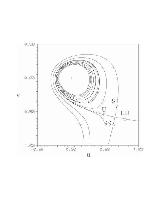
Figure 6: The nodal point - X point complex on the $(u,v)$ plane, in the adiabatic approximation when $t_{0}=10$ and $a=b=1$, $c=\sqrt{2}/2$.

Figure 6 shows how do the spirals emanating from the nodal point connect to the invariant manifolds emanating from the X-point in the adiabatic approximation. This figure is a numerical calculation of all the integral curves emanating from the X-point, when $a=b=1$, $c=\sqrt{2}/2$ and $t_{0}=10$. The X-point is found numerically up to twelve digits by looking for roots of Eqs.(4.1) close to the nodal point by a Newton-Raphson routine. The numerical solution $(u_{0},v_{0})$ is then inserted in the expressions for the matrix elements $a_{ij},i=1,2,j=1,2$, yielding the eigenvalues and eigenvectors of the variational matrix at $(u_{0},v_{0})$. Then, we give initial conditions for $u,v$ on both semi-lines (with respect to $(u_{0},v_{0})$) determined by the directions of the two eigenvectors, at a distance $10^{-4}$ from the X-point. Finally, we integrate numerically the differential equation:

$${du\over dv}=f_{uv}(u,v,t_{0})$$ (40)

found by dividing the two equations of (4.1), for each of the four different above sets of initial conditions. This yields numerically the two branches of the stable and unstable manifolds of the X-point. Clearly, since all the spirals terminating at the nodal point are described in the same sense, only one of these four branches can be connected to a spiral terminating at the nodal point. This branch can always be identified by comparing the senses of description of the manifolds and of the spiral. In particular, one of the asymptotic spirals of the nodal point is joined to one branch of the unstable manifold emanating from the X-point, if the nodal point is an attractor, or to the stable manifold, if the nodal point is a repellor. The set of all the integral curves of the flow in the neighborhood of the nodal point and X-point is hereafter called the ‘nodal point - X-point complex’.

Figure 7 shows a comparison of the spatial distribution of the nodal points (Fig.7a) and of the respective X-points (Fig.7b), on the plane $(x,y)$ when $a=b=1$, $c=\sqrt{2}/2$ and $t_{0}$ is in the interval $0\leq t_{0}\leq 1000$. The nodal lines and the X-point lines form similar patterns. In particular, similarly to the nodal points (section 2), the X-points avoid a central region of the plane $(x,y)$ in which the majority of orbits turn to be regular (subsection 4.3). Fig.7c shows the modulus of the positive eigenvalue of the X-point as a function of the distance $d_{0}$ of the X-point from the nodal point. We find numerically a power-law scaling $\lambda\propto 1/d^{p}$ with $p\simeq 1.5$, i.e., less steep than the theoretical scaling given by Eq.(39). From this figure, as well as from Figure 6, in which the distance of the X-point from the nodal point is about $d_{0}=0.9$, we deduce that the results obtained by the previous perturbative analysis are essentially valid not only at very small distances from the nodal point but also at relatively large distances (of order $10^{-1}$). At any rate, we always find that the stationary points of the vector field (4.1), as determined numerically, induce a similar phase-space structure as in Figure 6, i.e., this structure is general in the model considered.

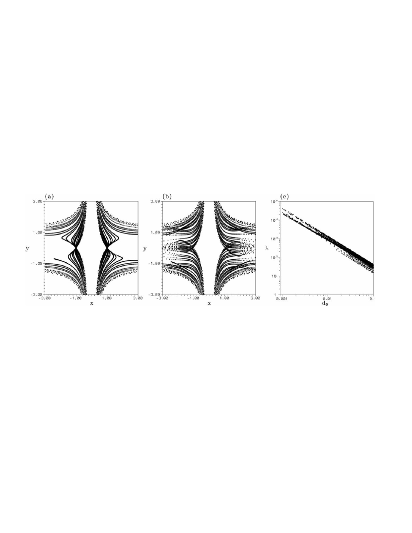
Figure 7: (a) Nodal lines, (b) X-point lines, and (c) the positive eigenvalue of the X-point versus the distance $d_{0}$ of the X-point from the nodal point, when $a=b=1$, $c=\sqrt{2}/2$.

4.2 The exponential sensitivity of the orbits

In order to understand how does the approach of an orbit to the nodal point - X-point complex introduce exponential sensitivity of the orbits to the initial conditions, we consider in detail the successive encounters of two nearby orbits, with initial separation $10^{-4}$, with this complex, which take place at snapshots at which the orbits pass close to the complex. To this end, we consider the orbit of Figure 8a (initial conditions $x_{1}(0)=y_{1}(0)=-1.1$ and $a=b=1$, $c=\sqrt{2}/2$) which has a number of consecutive encounters with the nodal point - X point complex. This orbit is chaotic, as seen from the calculation of the ‘finite time Lyapunov characteristic number’

$$\chi(t)={1\over t}\ln{|\xi(t)|\over|\xi(0)|}$$ (41)

where $\xi(t)\equiv(dx(t),dy(t))$ is the deviation vector associated with the orbit $(x_{1}(t),y_{1}(t))$, which is found by integrating the variational equations of motion together with the orginal equations of motion. The limit $\lim_{t\rightarrow\infty}\chi(t)$ yields the usual Lyapunov characteristic number. Numerically we find (Fig.8b) that this limit is close to $LCN\simeq 3\times 10^{-2}$. We then consider in detail the growth of deviations from this orbit by calculating also a nearby orbit $(x_{2}(t),y_{2}(t))$ with initial conditions $x_{2}(0)=x_{1}(0)+10^{-4}$, $y_{2}(0)=y_{1}(0)$.

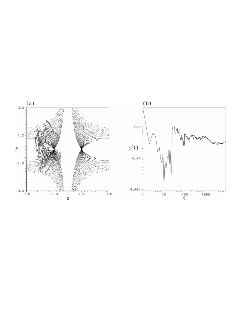
Figure 8: (a) Chaotic orbit with initial conditions $x(0)=y(0)=-1.1$, and $a=b=1$, $c=\sqrt{2}/2$. The orbit intersects the nodal lines of the left semiplane of $(x,y)$. (b) The ‘finite time’ Lyapunov characteristic number $\chi(t)$ for the same orbit. The limiting value is close to $LCN\simeq 0.03$.

Figure 9a shows the growth in time of the distance $\Delta S(t)=\bigg{(}(x_{1}(t)-x_{2}(t))^{2}+$ $(y_{1}(t)-y_{2}(t))^{2}\bigg{)}^{1/2}$ between the two nearby orbits. Clearly, the distance grows in general with time, but the growth takes place by rather abrupt steps. That is, while the distance has in general large fluctuations, there are particular times when the distance $\Delta S$ suddenly grows by jumps of about one order of magnitude (or more). Thus, the initial distance $\Delta S=10^{-4}$ becomes of order $10^{-3}$ at a time $t\simeq 25$, then of order $10^{-2}$ at $t\simeq 90$, and finally of order $10^{-1}$ (reaching even unity) at about $t\simeq 170$. After this time the distance $\Delta S$ can no longer be considered as small, that is, the orbits are no longer nearby.

Figure 9b is a close up to the third of the above described jumps, focusing on the time interval $160\leq t\leq 180$. From this figure it is clear that there are three encounters of the orbit with the nodal point - X point complex taking place in the considered time interval. In encounter (I), the minimum distance of the orbit (1) ($\equiv(x_{1}(t),y_{1}(t)$) from the nodal point is $\epsilon_{min}\simeq 0.4$, and the minimum distance from the X point is even smaller ($d_{min}\simeq 0.1$). On the contrary, in the next encounter (II), the minimum distance from the X-point is rather large ($d_{min}\simeq 0.9$) while the minimum distance from the nodal point is about the same as in case (I). Finally, in case (III) the minimum distance from the X-point is small ($d_{min}\simeq 0.2$) while the minimum distance from the nodal point is now large ($\epsilon_{min}\simeq 1$). Clearly, the growth of the distance $\Delta S$ mostly takes place during the encounters (I) and (III) in which the orbits pass closer to the X-point than to the nodal point. On the other hand, in the case of encounter (II), the growth is smaller while the orbit approaches closer the nodal point than the X-point. We conclude that large variations of $\Delta S$ are in general associated with approaches of the orbits to the X-point rather than to the nodal point.

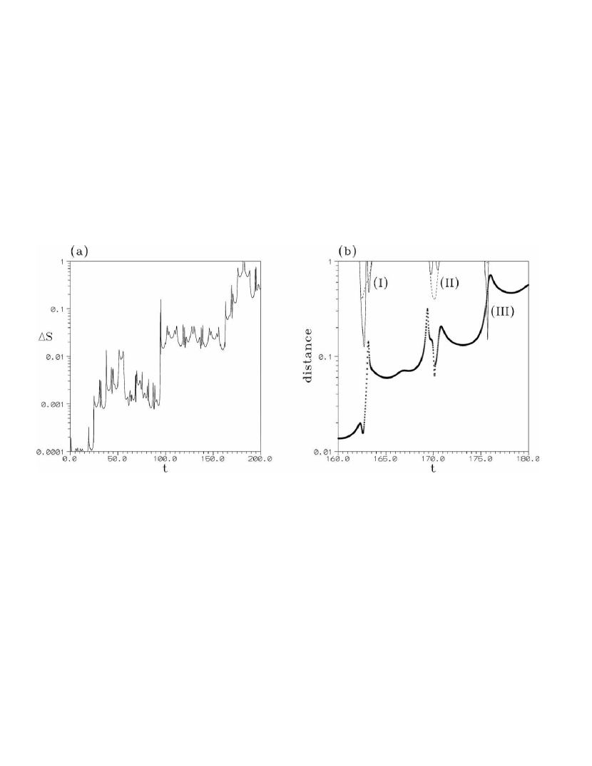
Figure 9: (a) The separation $\Delta S$ of two nearby orbits as a function of the time $t$ ($a=b=1$, $c=\sqrt{2}/2$ and initial conditions $x_{1}(0)=-1.1$, $x_{2}(0)=x_{1}(0)+10^{-4}$, $y_{1}(0)=y_{2}(0)=-1.1$). (b) A detail of (a) in the time interval $160\leq t\leq 180$. The line with thick dots gives $\Delta S$. The solid and dashed lines show the distances $d(t)$ and $\epsilon(t)$ of the orbit $(x_{1}(t),y_{1}(t))$ from the instantaneous locations of the X-point and of the nodal point respectively, when the latter are smaller than 1.

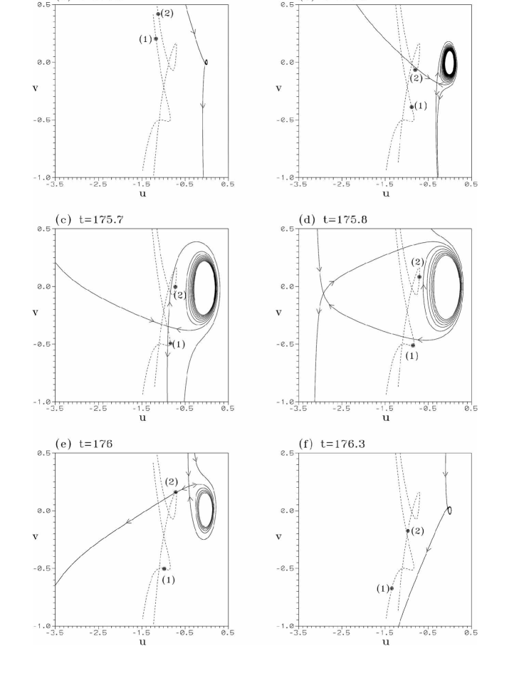
Figure 10: The encounter event (III) of Figure 9b viewed in detail in the plane $(u,v)$. The orbits (1)and (2), in the time interval $175\leq t\leq 176.5$, are shown by dashed lines, while the thick dots indicate the positions of the orbital points on these lines at the times (a) $t=175.2$, (b) $t=175.5$, (c) $t=175.7$, (d) $t=175.8$, (e) $t=176$, and (f) $t=176.3$. The invariant manifolds of the instantaneous X-point - nodal point complex are plotted for the same times. The main deflection of the orbits, takes place within the time interval $175.7\leq t\leq 175.8$.

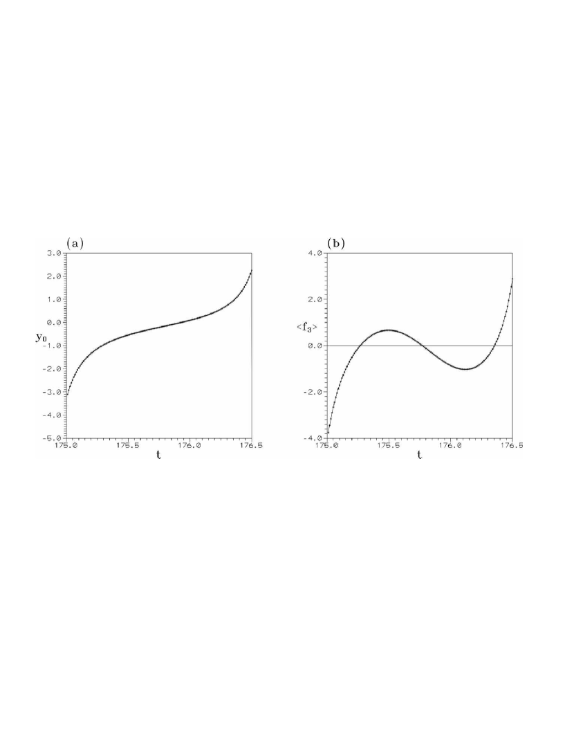
Figure 11: (a) The nodal point coordinate $y_{0}(t)$ in the time interval $175\leq t\leq 176.5$. (b) The value of $<f_{3}>(t_{0})$ in the time interval $175\leq t_{0}\leq 176.5$. There are three moments in this interval at which $<f_{3}>=0$. These correspond to changes in the topological structure of the X-point - nodal point complex.

Figure 10 shows in detail how does the separation of the orbits take place during the encounter event (III). The two nearby orbits are shown as dashed curves, in the time interval $175\leq t\leq 176.5$, in the moving frame of reference centered at the nodal point. The different frames correspond to different time snapshots, and the particular positions of the orbital points $(1)\equiv(u_{1},v_{1})=(x_{1}-x_{0},y_{1}-y_{0})$, $(2)\equiv(u_{2},v_{2})=(x_{2}-x_{0},y_{2}-y_{0})$ at the given snapshot are marked with thick dots. Finally, the instantaneous stable and unstable asymptotic manifolds emanating from the X-point (in the adiabatic approximation) are plotted for the time corresponding to each frame.

We notice that the X-point changes position relative to the nodal point, which in these frames is always centered at $(u,v)=(0,0)$. In fact, as already mentioned, the two points collide whenever $\sin(1+c)t=0$ (and then $y_{0}=\pm\infty$). There are two consecutive collisions at $t=174.829$ and $t=176.669$. The time $t=175.2$ (Fig.10a) is close to the first of the above two collision times and, consequently, the X-point at $t=175.2$ is very close to the nodal point. Then, the X-point moves to the left up to about $t=175.8$ (Figs.10b,c,d), and then it returns to the right approaching again the nodal point (Figs.10e,f). The time $t=176.3$ is close to the second collision time ($t=176.669$), thus the X-point in Fig.10f comes again very close to the nodal point.

Now, at the time $t=175.2$ the orbits have a separation of about $\Delta S=0.15$ (Fig.10a). At this time snapshot the orbits move in a nearly parallel way, and their distances from both the nodal point and X-point are rather large (of order unity). The orbits move downwards in about the same direction as indicated by the arrows of the invariant manifolds of the X-point (in the rest frame $(x,y)$ this means that the nodal point approaches the orbital points from $y=-\infty$, see also Fig.11a). Furthermore, as the X-point itself moves from right to left, both orbits approach to it (Fig.10b, $t=175.5$).

The crucial phenomenon occurs near $t=175.7$ (Fig.10c). Around this time, the X point crosses a segment joining the orbital points (1) and (2). The two points have approached the moving X-point at a distance smaller than $0.2$, but they are on opposite branches of the unstable manifold. Thus, point (1) moves downwards following one branch of the unstable manifold of the X point, while point (2) moves upwards following the other branch of the same manifold. This causes a abrupt growth of the distance of the two points by a factor $\simeq 3$.

An important change in the topological structure of the invariant manifolds, that influences the orbits, takes place between $t=175.7$ (Fig.10c) and $t=175.8$ (Fig.10d). Namely, at $t=175.7$ (Fig.10c) the spiral terminating at the nodal point is connected to one branch of the stable manifold of the X-point, while at $t=175.8$ (Fig.10d) it is connected to one branch of the unstable manifold of the X-point. This transition takes place via a Hopf bifurcation which is described in detail below. At any rate, at $t=175.8$ (Fig.10d) the X-point has moved to the left, far from the nodal point, and orbit (1) is close to the stable manifold of the X-point. Thus, orbit (1) is deflected to the left, while orbit (2) continues slowly upwards.

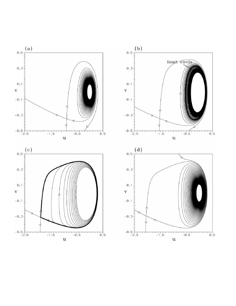
Figure 12: The instantaneous flow chart of the X-point - nodal point complex at the times (a) $t_{0}=176.7$, (b) $t=176.76$, (c) $t=176.7750938$, (d) $t=175.78$. A Hopf bifurcation taking place near the value $t=176.72$ (at which $<f_{3}>=0$ in figure 11), leads to the formation of a limit circle (repellor), shown in (b), which disappears after reaching the separatrix of (c).

Finally, a little later ($t=176$, Fig.10e), the X-point returns close to the nodal point so that point (2) comes very close to the unstable manifold of the X-point. This causes a deflection of orbit (2) to the left, while orbit (1), although far from the X-point - nodal point complex, moves also to the left, following the general direction of motion indicated by the unstable manifold of the X-point. Finally, at $t=176.3$ (Fig.10f) both orbital points are far from the X-point - nodal point complex, but they are relatively close to the unstable manifold of the X-point in a downwards direction. From there on both orbits move in a nearly parallel way until the next encounter event which occurs much later. The overall growth of the distance of the two orbits by a factor 3 in a time $\Delta t=176.3-175.2=1.1$ corresponds to an exponential growth rate $\ln 3/1.1\simeq 1$ in this time interval. This is much larger than the average exponential growth rate (=LCN$\simeq 0.03$) for the same orbit within a much longer time interval. This fact justifies the statement that the growth of $\Delta S$ is by abrupt jumps, which take place during local (in space and time) encounters with the nodal point - X-point complex.

The topological transition in the phase space structure taking place between $t=175.7$ (Fig.10c) and $t=175.8$ (Fig.10d) is due to a Hopf bifurcation taking place between these two times as a result of the fact that the value of $<f_{3}>$ (Eq.(35)) changes sign (Fig.11b), while the sign of $d\phi/dt$ remains constant (because there is no change in the sign of $\sin(1+c)t$, i.e., no transition of $y_{0}$ to infinity, in the same interval, Fig.11a). By virtue of Eq.(36), the change of the sign of $<f_{3}>$ at a time between $t_{0}=175.7$ and $t_{0}=175.8$ implies that the nodal point turns from repellor to attractor. The precise time when this happens depends on higher order terms in the development of the equations of motion around the nodal point, but it is nevertheless close to the time when the term depending on $<f_{3}>$ becomes equal to zero. Numerically, we find the bifurcation to take place near $t_{0}=175.75$. Before this time (e.g. at $t_{0}=175.7$, Fig.12a) the nodal point is a repellor, and a spiral emanating from it joins the stable manifold of the X-point. On the other hand, a little after this time ($t_{0}=175.76$, Fig.12b), the nodal point has become an attractor, while the stability character of the X-point does not change appreciably. Thus, between the nodal point and X-point there is now a limit circle which acts as a repellor, i.e., the orbits on both sides of the circle move away from it on spirals either terminating at the nodal point or moving towards the X-point. In the latter case a spiral either joins the stable manifold terminating at the X-point or continues downwards, away from the X-point, in the channel formed between the two branches of the unstable manifold of the X-point (Fig.12b). As $t_{0}$ increases the limit circle moves outwards approaching the invariant manifolds of the X-point. At a critical time $t_{0}=175.7750938$ (Fig.12c) the limit circle coincides with the invariant manifolds of the X-point. At still larger times ($t=175.78$, Fig.12d), the limit circle disappears and one branch of the unstable manifold of the X-point continues now as a spiral terminating at the nodal point.

Figure 13 shows how does the effect of a close encounter of an orbit with the nodal point - X point complex shows up in the time evolution of the deviations $\xi(t)$ as given by solving the variational equations of motion together with the equations of motion for one orbit. The abrupt jumps in the length of the deviation vector $\mathbf{\xi}=(dx,dy)\equiv(du,dv)$ (Fig.13a) are associated with passages of the orbit close to the nodal point - X-point complex. In order to obtain quantitative estimates of the exponential growth of deviations at successive encounter events, we proceed as follows: The time span of the total run of an orbit is split in short windows of width $\Delta t=0.1$ (the timestep of the numerical integration is variable and much shorter than this window, i.e., $dt\leq 10^{-5}$). In each time window, an average ‘stretching number’ (Voglis and Contopoulos 1994) is calculated according to:

$$a_{i}={1\over\Delta t}\ln|{\xi(t_{i}+\Delta t)\over\xi(t_{i})}|$$ (42)

where $t_{i}=(i-1)\times\Delta t$ is the initial time of the i-th window, and $\xi(t)$ is the length of the deviation vector $\mathbf{\xi}(t)$ at the time $t$. This quantity characterizes the local growth rate of deviations, while the average value of all the stretching numbers yields the ‘finite time Lyapunov characteristic number’

$$\chi(t)={1\over N\Delta t}\sum_{i=1}^{N}\ln|{\xi(t_{i}+\Delta t)\over\xi(t_{i})}|={1\over t}\ln|{\xi(t)\over\xi(0)}|~{}~{}.$$ (43)

(The limit $\lim_{t\rightarrow\infty}\chi(t)$ defines the Lyapunov characteristic number of the orbit). In the same time windows we also store the values of the minimum distance of the orbit to the nodal point $\epsilon_{min}$, and to the X-point $d_{min}$, as well as the minimum distance between the X-point and nodal point $d_{0,min}$. These three minimum values are not occurring at precisely the same times within a given time window, however the width of the window $\Delta t=0.1$ itself is small enough so that the occurrences of the minimum values can be considered as nearly simultaneous.

Figure 13b then shows the main result. The distances that an orbit reaches from either the nodal point or the X-point, for all the 10000 time windows in a total time span $0\leq t\leq 1000$, are grouped in bins of width $\delta=2.5\times 10^{-2}$. The abscissa in Fig.13b gives the median value of each bin, which is the same for either the distance $d$ from the X-point or $\epsilon$ from the nodal point. A weighted average value $\bar{a}$ of the stretching number is then calculated in each bin, by summing the values of the stretching numbers which appear during all the passages of the orbit at distances $d\pm\delta/2$ from the X-point, or $\epsilon\pm\delta/2$ from the nodal point, and dividing by the total number of values of the stretching number in the sample. Clearly, when the stretching numbers are grouped with respect to the various distances $d$ reached from the X-point, the average stretching number $\bar{a}(d)$ is positive for all distances $d\leq 0.25$, while for $d>0.25$, $\bar{a}(d)$ fluctuates between positive and negative values, showing nevertheless a preference for positive values. Such a preference reflects the hyperbolic dynamics induced on the orbits by their approaches to the X-point. That is, the general solution of the variational equations close to the X-point contains terms growing exponentially and other terms decaying exponentially. However, the growing terms prevail as the time $t$ increases. Thus, the overall average stretching number $<\bar{a}>$ after many encounters of an orbit with the X-point turns to be positive.

On the other hand, when the stretching numbers are grouped with respect to the distance $\epsilon$ of an orbit from the nodal point, the average stretching number $\bar{a}(\epsilon)$ (dashed curve in Fig.13b) shows no clear preference towards positive or negative values when $\epsilon$ is small ($\epsilon<0.25$), while a preference towards positive values of $\bar{a}$ appears when $\epsilon>0.25$. This agrees with Fig.13a, or Fig.9b, which show that the growth of deviations occurs mainly during encounters (I) and (III), during which the minimum distance of the orbit from the X-point is smaller than the distance from the nodal point.

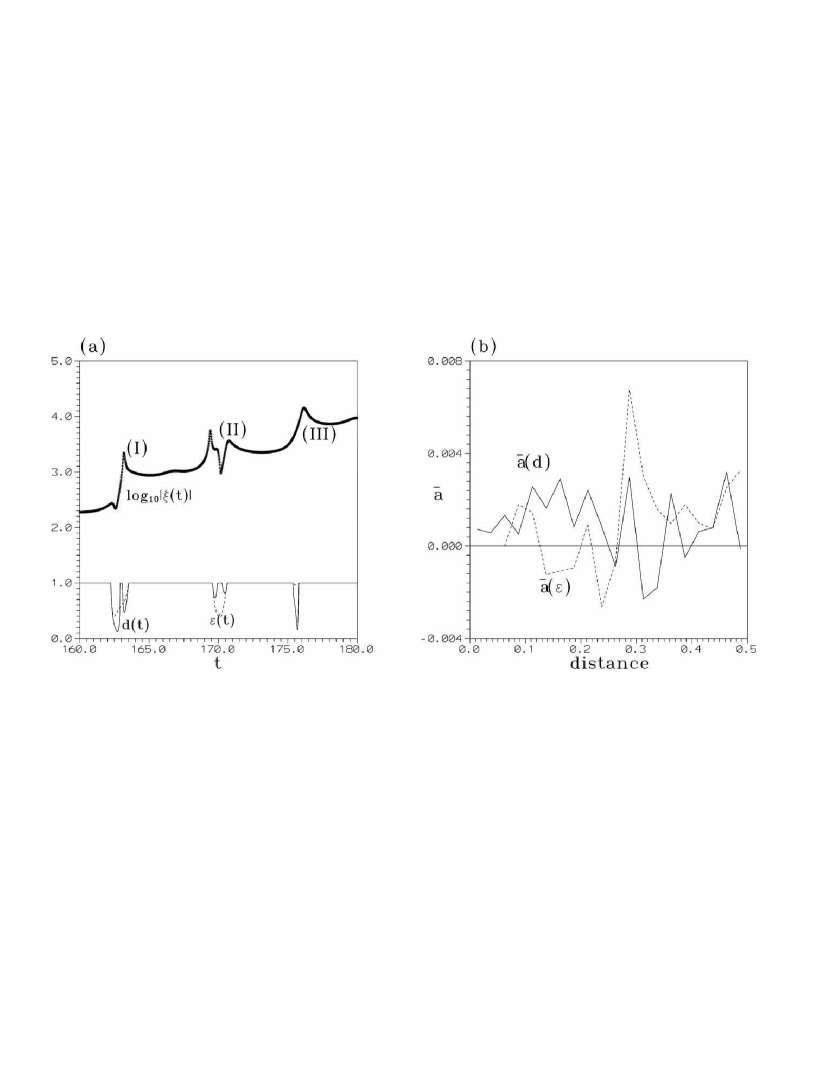
Figure 13: (a) the growth of the length of the deviation vector $\xi(t)$ for the same orbit $(x_{1}(t),y_{1}(t))$ as in Figure 9b. The lower solid and dashed lines are the same as in Fig.9b. (b) The mean stretching number $\bar{a}$ as a function of the distance from the X-point $\bar{a}(d)$, or from the nodal point $\bar{a}(\epsilon)$, for the same orbit and time up to $t=1000$. For each value of $d$ or $\epsilon$, the value of $\bar{a}$ is calculated by taking the sum of all the stretching numbers (Eq.(42) with $\Delta t=0.1$) occuring at passages of the orbit at a distance $d\pm\delta/2$ from the X-point and $\epsilon\pm\delta/2$ from the nodal point respectively, with $\delta=2.5\times 10^{-2}$.

5 Discussion

The role of the nodal points of the wavefunction (sometimes called ‘quantum vortices’) in determining the main features of the ‘hydrodynamical’ probability flow has been studied in a number of different quantum systems (see Wyatt (2005) and references therein). Here we refer only to studies related to our own, i.e., to the appearance of chaos due to nodal points (quantum vortices).

Berry (2005) studied the flow lines of a general time-independent complex scalar field $\psi(x,y)$ and found that they typically spiral in or out of a ‘phase vortex’. He also found the stationary points of this flow which can be either elliptic or hyperbolic. Berry explicitly excludes a spiral flow near the vortices of the Schrödinger field because the quantum mechanical current satisfies $\nabla\cdot\mathbf{j}=0$. This is precisely what happens in our case if one considers the flow lines in the rest frame $(x,y)$ rather than a frame moving together with the nodal points. In the rest frame, the flow integral curves (found by dividing by parts Eqs.(4)) are given by the differential equation:

$${dy\over dx}={bc^{1/2}x\big{(}ax\sin ct+\sin(1+c)t\big{)}\over a\sin t+bc^{1/2}y\sin(1+c)t}~{}~{}.$$ (44)

Keeping the time $t$ frozen in the r.h.s., Eq.(44) yields the integral curves

$$a\sin ty+bc^{1/2}\sin(1+c)t{y^{2}\over 2}-abc^{1/2}\sin ct{x^{3}\over 3}-bc^{1/2}\sin(1+c)t{x^{2}\over 2}=C$$ (45)

The critical points of (45) are given by the solutions of $\nabla C=0$. There are two solutions:

$$(x_{1},y_{1}) = (-{\sin(1+c)t\over a\sin ct},-{a\sin t\over bc^{1/2}\sin(1+c)t})\equiv(x_{0},y_{0})$$

$$(x_{2},y_{2}) = (0,-{a\sin t\over bc^{1/2}\sin(1+c)t})\equiv(0,y_{0})~{}~{}.$$ (46)

The first critical point $(x_{1},y_{1})$ coincides with the nodal point. The eigenvalues of the Hessian matrix of $C$ at $(x_{0},y_{0})$ are given by $\lambda_{1,2}=\pm ibc^{1/2}\sin(1+c)t$, thus they are imaginary at any time $t$, implying that the integral curves of the velocity field in the neighborhood of the nodal point are approximately ellipses centered at $(x_{0},y_{0})$ at any time $t$ except $t_{c}=2k\pi/(1+c)$ or $t_{c}=(2k+1)\pi/(1+c)$ with $k$ integer. The difference with respect to the approximation of Eq.(36) is that in the moving frame of reference the instantaneous flow lines form spirals if $<f_{3}>\neq 0$, i.e., if $\dot{x}_{0}\neq 0$ or $\dot{y}_{0}\neq 0$, that is the spirals appear (in the moving frame) only because the velocity of the nodal point is non-zero. Furthermore, in our analysis, the eigenvalues of the X-point in the nodal point - X-point complex scale as an inverse power of the distance of the X-point from the nodal point. On the contrary, the eigenvalues of the second critical point $(x_{2},y_{2})$ of Eqs.(5) are given by $\lambda_{1,2}=\pm bc^{1/2}\sin(1+c)t$, i.e. they are bounded by quantities of order $a$ or $b$. Thus, despite the fact that $(x_{2},y_{2})$ represents also a saddle point in the rest frame of motion in the adiabatic approximation, its influence to the dynamics is not so important when $a$ and $b$ are of order unity. In fact, this point is always attached to the y-axis, so that it can only influence the deviation vectors at times when the orbits come close to this axis. This is at variance with the numerical results showing that positive stretching numbers are introduced when the orbits approach the nodal point - X-point complex at arbitrary locations within the plane $(x,y)$.

Wisniacki and Pujals (2005) studied the Bohmian orbits in an example similar to ours, namely the superposition of three stationary states of the double harmonic oscilator, when, however, the latter is isotropic ($c=1$) and the ratios of the probability amplitudes of the states $|\Psi_{10}>$ and $|\Psi_{11}>$ with that of $|\Psi_{00}>$ are complex. In the case $c=1$ there is only one fundamental frequency of the time-dependent trigonometric terms of the equations of motions. This allows one to obtain stroboscopic plots of the orbits, i.e., Poincaré surfaces of section. Wisniacki et al. pointed out that it is the motion of the nodal point which generates chaos. However, their mechanism of introduction of chaos is different from ours. Namely, in the case of Wisniacki et al. the motion of the nodal point generates a saddle point on the surface of section, but the surface of section is area preserving, and the transverse intersections between the stable and unstable invariant manifolds of the saddle point generate homoclinic chaos. The most important difference is that their mechanism can be applied only in resonant cases while our mechanism applies to general non-resonant cases.

A similar example was studied by Makowski et al. (2000). Both results correspond to the case of a complex ratio $a/b$ and $c=1$. On the other hand, if $c$ is rational but $a/b$ is real, all the orbits are periodic and neutrally stable, thus there is no chaos at all (some examples of seemingly chaotic orbits in a similar model given by Konkel and Makowski (1998), for a rational value of $c$, are just due to numerical errors caused by the stiffness of the equations of motion close to the X-point. In order to obtain the correct orbits, which are periodic and not chaotic, we had to use a program in Mathematica with an accuracy of 50 digits!).

Falsaperla and Fonte (2003) studied the orbits near nodal lines in a 3D model. In that case the orbits describe helical motions around the nodal line (called by these authors ‘spirals’) while the projections of the motion on a $z=$constant surface are ellipses. These authors point out that the nodal lines “regularize the motion” in their neighborhood, and only orbits not following a definite nodal line are “intermittent chaotic”. They furthermore find too that the period of rotation along the helix is of order $O(\epsilon^{2})$, where $\epsilon$ in this case is the distance from the nodal line. While a detailed comparison of 2D and 3D models is necessary, our analysis above shows essentially why the growth of the deviation vectors is intermittent, i.e., it takes place by abrupt steps whenever an orbit approaches the nodal point - X-point complex. Furthermore, we also explain why the appearance of chaos is not strictly correlated with very close approaches to the nodal point (in such cases the orbits simply spiral around the nodal point), but it occurs mainly when the orbit approaches closely the X-point associated with the nodal point. This happens even if the latter has a distance from the nodal point which is much larger than the distance of the orbit from the X-point.

Wu and Sprung (1999) gave plots (their Fig.4) of the probability flow, which resemble our Figure 7. However, this resemblence is only due to a ‘phase mixing’ phenomenon taking place in the rest frame near the nodal point. Namely, because the rotation frequency depends on the distance from the nodal point as $1/\epsilon^{2}$, a fluid element of some thickness approaching the nodal point forms a number of windings around the nodal point due to the differential rotation of the orbits included in its area. These windings give the impression of forming a spiral pattern, which is, however, only apparent, namely the windings are limited by an inner circle (or ellipse) due to orbits of the fluid element closest to the nodal point (this is different from our limit circle of Fig.12). On the other hand, in earlier works the same authors found spiral motions around quantum vortices in the rest frame of motion, when the quantum system is subject to a vector potential in addition to a scalar potential (Wu and Sprung 1994). The plots shown in that work are similar to ours, although the similarity in the topological structure of the phase space is due to the presence of an extra term in the equations of motion due to the vector potential, rather than to the motion of the nodal point.

Finally, Frisk (1997) and Wisniacki et al. (2006) noticed that the transition to chaos is enhanced when there are many co-existing vortices influencing the orbits. In that case it is necessary to consider the connections of the invariant manifolds emanating from the stationary points of one vortex with those of other vortices and see how this can increase chaos and transport phenomena in configuration space. This problem is proposed for future study.

6 Conclusions

In summary, the main conclusions of our study are the following:

1) In a simple quantum system consisting of the superposition of three eigenstates of the double harmonic oscillator potential, in which there is one nodal point of the wavefunction travelling in the plane $(x,y)$, we proved the existence of domains of this plane which are free of nodal points. Bohmian orbits in these domains, as well as orbits slightly overlapping with the nodal lines, are regular.

2) In the central domain devoid of nodal lines the equations of motion admit expansions in powers of the probability amplitudes of the eigenstates, yielding the trajectories as double Fourier series in the fundamental frequencies of the system. These series represent theoretical orbits which are, by definition, regular. We show the agreement of the theoretical and numerical orbits in this domain for sufficiently small values of the probability amplitudes and sufficiently high order of the expansions, and use this to explain the morphological characteristics of the regular orbits.

3) Close to the nodal points, we use different expansions, in powers of the distance from the nodal point, in order to unravel the dynamics. The angular frequency of motion in a $\epsilon-$ neighborhood of the nodal point is of order $O(1/\epsilon^{2})$. This justifies the use of the adiabatic approximation. In the fixed frame $(x,y)$ the flow lines close to the nodal point are ellipses. However, in a moving frame attached to the nodal point, the flow lines are spirals terminating at the nodal point. The temporary sense of description of the spirals by the orbits is unique, i.e., at a given time the nodal point is either an attractor or a repellor. Furthermore, at a finite distance from the nodal point there is a saddle stationary point of the flow with one asymptotic manifold joining the spiral and the other three extending to infinity.

4) The eigenvalues of the X-point scale as $1/d_{0}^{p}$ where $d_{0}$ is the distance of the X-point from the nodal point and $p\simeq 2$. Furthermore, the distance $d_{0}$ can be arbitrarily small, i.e., there are collisions of the X- and nodal points. We show that the orbits approaching close to the X-point exhibit exponential growth of their deviations, i.e., they are chaotic. In all numerical examples we find that chaos is associated with the approach of the orbits to the X-point, which, however, is only guaranteed when we have a moving nodal point. Furthermore the chaotic influence of the X-point on the orbits is strongest when the X-point is closest to the nodal point. Thus, the nodal point indirectly influences the transition of Bohm’s trajectories from order to chaos via the above mechanism.

7 Appendix: Calculation of $<f_{3}>$

The precise form of Eq.(30) reads:

$${dR\over d\phi}=\frac{-AR^{2}-\dot{x}_{0}G\cos\phi-\dot{y}_{0}G\sin\phi}{B-CR-\dot{y}_{0}{G\over R}\cos\phi+\dot{x}_{0}{G\over R}\sin\phi}$$ (47)

where

$$A=abc^{1/2}\cos^{2}\phi\sin\phi\sin ct,~{}~{}B=bc^{1/2}\sin(1+c)t,~{}~{}C=abc^{1/2}\cos^{3}\phi\sin ct$$

and $G=g_{2}R^{2}+g_{3}R^{3}+g_{4}R^{4}$ with

$$g_{2}={\cos^{2}\phi\over x_{0}^{2}}-2bc^{1/2}\sin\phi\cos\phi\cos(1+c)t+b^{2}cx_{0}^{2}\sin^{2}\phi$$

$$g_{3}=-{2bc^{1/2}\over x_{0}}\cos(1+c)t\cos^{2}\phi\sin\phi+2b^{2}cx_{0}\cos\phi\sin^{2}\phi$$

$$g_{4}=b^{2}c\cos^{2}\phi\sin^{2}\phi~{}~{}.$$

Expanding Eq.(47) in ascending powers of $R$ we find:

$${dR\over d\phi} = \Bigg{(}-AR^{2}-\dot{x}_{0}g_{2}\cos\phi R^{2}-\dot{x}_{0}g_{3}\cos\phi R^{3}-\dot{y}_{0}g_{2}\sin\phi R^{2}-\dot{y}_{0}g_{3}\sin\phi R^{3}\Bigg{)}$$ (48)

$$\times {1\over B}\Bigg{(}1+{c\over B}R+\dot{y}_{0}{g_{2}\over B}\cos\phi R-\dot{x}_{0}{g_{2}\over B}\sin\phi R\Bigg{)}+\ldots$$

Averaging Eq.(48) we find:

$${d\bar{R}\over d\phi}={1\over 2\pi}\int_{0}^{2\pi}{dR\over d\phi}d\phi=<f_{2}>R^{2}+<f_{3}>R^{3}+...$$ (49)

where

$$f_{2}={1\over B}(-A-\dot{x}_{0}g_{2}\cos\phi-\dot{y}_{0}g_{2}\sin\phi)$$

$$f_{3}={1\over B}(-A-\dot{x}_{0}g_{2}\cos\phi-\dot{y}_{0}g_{2}\sin\phi)\times({c\over B}+\dot{y}_{0}{g_{2}\over B}\cos\phi-\dot{x}_{0}{g_{2}\over B}\sin\phi)$$

$$+{1\over B}(-\dot{x}_{0}g_{3}\cos\phi-\dot{y}_{0}g_{3}\sin\phi)~{}~{}.$$

Collecting terms of the form

$${1\over 2\pi}\int_{0}^{2\pi}\cos^{n}\phi\sin^{m}\phi d\phi,~{}~{}~{}m,n~{}~{}\mbox{even}$$

we find that $<f_{2}>=0$, while

$$<f_{3}> = {1\over 16b^{2}c\sin^{2}(1+c)t_{0}}\Bigg{(}4abc^{1/2}\sin ct(-{\dot{x}_{0}\over x_{0}^{2}}+b^{2}c\cos(1+c)t\dot{y}_{0})$$ (50)

$$+4\dot{x}_{0}\dot{y}_{0}(b^{4}c^{2}x_{0}^{4}-{1\over x_{0}^{4}})-4bc^{1/2}\cos(1+c)t(\dot{x}_{0}^{2}-\dot{y}_{0}^{2})({1\over x_{0}^{2}}+b^{2}cx_{0}^{2})\Bigg{)}$$

$$+{bc^{1/2}\over 4bc^{1/2}\sin(1+c)t_{0}}\Bigg{(}{\dot{y}_{0}\cos(1+c)t_{0}\over x_{0}}-bc^{1/2}x_{0}\dot{x}_{0}\Bigg{)}$$

which after some simplification yields Eq.(35).

References

- [1] Beenakker, C.W., and van Houten, H.: 1991, Solid State Phys. 44, 1.
- [2] Berry, M.V.: 2005, J. Phys. A, 38, L745.
- [3] Bohm, D.: 1952a, Phys. Rev. 85, 166.
- [4] Bohm, D.: 1952b, Phys. Rev. 85, 180.
- [5] Bohm, D and Hiley, B.J.: 1993, “The Undivided Universe”, Routhledge, London.
- [6] Bohm, D., and Vigier, J.P.: 1954, Phys. Rev. 26, 208.
- [7] Contopoulos, G.: 1960, Z. Astrophys. 49, 273.
- [8] Cushing, J.T.: 2000, Philosophy of Science 67, S432.
- [9] de Broglie, L.: 1926, Nature 118, 441.
- [10] de Polavieja, G.G.: 1996, Phys. Rev. A, 53, 2059.
- [11] de Sales, J.A. and Florencio, J.: 2003, Phys. Rev. E, 67, 016216.
- [12] Dewdney, C., Holland, P.R., and Kyprianidis, A.: 1986, Phys. Lett. A 119, 259.
- [13] Dewdney, C., and Malik, Z.: 1996, Phys. Lett. A 220, 183.
- [14] Dürr, D., Goldstein, S., and Zanghi, N: 1992, J. Stat. Phys. 68, 259.
- [15] Efthymiopoulos, C., and Contopoulos, G.: 2006, J. Phys. A 39, 1819.
- [16] Faisal, F.H.M., and Schwengelbeck, U.: 1995, Phys. Lett. A, 207, 31.
- [17] Falsaperla, P., and Fonte, G.: 2003, Phys. Lett. A, 316, 382.
- [18] Feit, M.D., and Fleck, J.A.: 1984, J. Chem. Phys. 80, 2578.
- [19] Feynman, R.P., Leighton, R.B., Sands, M: 1963, ‘The Feynman Lectures in Physics’, v.3, Ch.21, Addison-Wesley, New York.
- [20] Frisk, H.: 1997, Phys. Lett. A 227, 139.
- [21] Hirschfelder, J., Christoph, A.C., and Palke, W.E.: 1974, J. Chem. Phys. 61, 5435.
- [22] Holland, P.: 1993, “The Quantum Theory of Motion”, Cambridge University Press, Cambridge.
- [23] Holland, P.: 2005, Annals of Physics, 315, 505.
- [24] Iacomelli, G., and Pettini, M.: 1996, Phys. Let. A 212, 29.
- [25] Konkel, S., and Makowski, A.J.: 1998, Phys. Lett. A 238, 95.
- [26] Lopreore,C.L., and Wyatt, R.E.: 1999, Phys. Rev. Lett. 82, 5190.
- [27] Madelung, E.: 1926, Z.Phys. 40, 332.
- [28] Makowski, A.J., Peplowski, P., and Dembinski, S.T.: 2000, Phys. Lett. A, 266, 241.
- [29] Parmenter, R.H. and Valentine, R.W.: 1995, Phys. Lett. A, 201, 1.
- [30] Parmenter, R.H., and Valentine, R.W.: 1996, Phys. Lett. A 213, 319.
- [31] Philippidis, C., Dewdney, C., and Hiley, B.J.: 1979, Nuovo Cim. B 52, 15.
- [32] Skodje, R.T., Rohrs, H.W., and VanBuskirk, J.: 1989, Phys. Rev. A, 40, 2894.
- [33] Valentini, A., and Westman, H.: 2005, Proc. R. Soc. A, 461, 253.
- [34] Verhulst, F: 1993, “Nonlinear differential equations and dynamical systems”, Springer-Verlag, Heidelberg - Berlin.
- [35] Wisniacki, D.A., and Pujals, E.R.: 2005, Europhys. Lett., 71, 159.
- [36] Wisniacki, D.A., Pujals, E.R., and Borondo, F.: 2006, Europhys. Lett., 73, 671.
- [37] Wu, H., and Sprung, D.W.L.: 1999, Phys. Lett. A, 261, 150.
- [38] Wyatt, R.E.: 2005, ‘Quantum Dynamics with Trajectories: Introduction to Quantum Hydrodynamics’, Springer, New York.