Selfconsistent gauge-invariant theory of in-plane infrared response of high-T_c cuprate superconductors involving spin fluctuations

Abstract

We report on results of our theoretical study of the in-plane infrared conductivity of the high-$T_{c}$ cuprate superconductors using the model where charged planar quasiparticles are coupled to spin fluctuations. The computations include both the renormalization of the quasiparticles and the corresponding modification of the current-current vertex function (vertex correction), which ensures gauge invariance of the theory and local charge conservation in the system. The incorporation of the vertex corrections leads to an increase of the total intraband optical spectral weight (SW) at finite frequencies, a SW transfer from far infrared to mid infrared, a significant reduction of the SW of the superconducting condensate, and an amplification of characteristic features in the superconducting state spectra of the inverse scattering rate $1/\tau$. We also discuss the role of selfconsistency and propose a new interpretation of a kink occurring in the experimental low temperature spectra of $1/\tau$ around $1000\>\mathrm{cm}^{-1}$.

I INTRODUCTION

Most of the existing calculations of the frequency dependent conductivity $\sigma$ in high-$T_{c}$ cuprate superconductors (for representative examples see Refs. Quinlan:1996:PRB, ; Schachinger:1997:PRB, ; Munzar:1999:PhysicaC, ; Carbotte:1999:Nature, ; Abanov:2001:PRB, ; Casek:2005:PRB, ; Hwang:2007:PRB, ) employ the approximation, where interactions of the excited states are not taken into account, i.e., the so called vertex corrections (VC) in the perturbation expansion for $\sigma$ are neglected. It is well known that this approach is not gauge invariant and the results may depend on the gauge of the vector and scalar potentials. Physically, gauge invariant response is a manifestation of local charge conservation in the system. We recall that the usual restricted conductivity sum rule for the normal state (NS)

$$I_{f}=-({\pi e^{2}}/{2\hbar^{2}})K\;,$$ (1)

where

$$I_{f}=\int_{0^{+}}^{\infty}\sigma_{1x}(\omega)\mathrm{d}\omega$$ (2)

is the intraband optical spectral weight and

$$K=-\frac{1}{V}\sum_{\bm{k}\alpha}\frac{\partial^{2}\varepsilon_{\bm{k}}}{\partial k_{x}^{2}}n_{\bm{k}\alpha}$$ (3)

the so called effective kinetic energy per unit cell ($\alpha$ stands for the spin index, $\varepsilon_{\bm{k}}$ is the dispersion relation, and $n_{\bm{k}\alpha}$ the occupation factor), is a consequence of the gauge invariance Nozieres:1999:book . For concreteness we have considered the conductivity along the $x$-axis. The NS conductivity calculated using a no-VC approach need thus not satisfy the sum rule. Similarly, for the superconducting state (SCS), the spectral weight of the condensate $I_{c}$, which is given by

$$I_{f}+I_{c}=-({\pi e^{2}}/{2\hbar^{2}})K\;,$$ (4)

as obtained within a no-VC calculation, may be rather different from that of the corresponding gauge-invariant approach. These possible problems call for an assessment of the contribution of the relevant VC to $I_{f}$.

Another reason for studying the VC has been highlighted by Millis and coworkers. If the VC were negligible, the infrared (IR) conductivity would be determined solely by the quasiparticle selfenergy, that can be, at least in principle, extracted from photoemission data. Millis and Drew Millis:2003:PRB found out, however, that the effective scattering rate in optimally doped Bi₂Sr₂CaCu₂O_8+δ obtained using the selfenergy estimated from the photoemission data, is much higher than the value resulting from the IR data. Similarly, Millis et al. Millis:2005:PRB demonstrated that the local selfenergy obtained by fitting (without VC) the IR data of thin films of Pr_2-xCe_xCuO_4+δ leads to much lower (by a factor of 3-4) values of the quasiparticle velocity than observed by photoemission. These discrepancies appear to imply the presence of large VC.

A brief account of the VC to the NS conductivity of cuprate superconductors has been given by Monthoux and Pines in one of the pioneering papers on the nearly antiferromagnetic Fermi liquid (NAFL) model Monthoux:1994:PRB . For this particular model, the VC have been found to cause a slight increase (about 20%) of resistivity. Current vertex renormalization within the conserving fluctuation exchange (FLEX) approach Manske has been systematically investigated by Kontani and coworkers (see, e.g., Refs. Kontani:2006:JPSJ, and Kontani:2005:condmat, and references therein). They successfully explained the anomalous temperature dependence of the Hall conductivity in cuprates and estimated the contribution of the VC to the normal state conductivity. Benfatto et al.Benfatto:2005:PRB and Aristov and Zeyher Aristov:2005:PRB discuss the role of the VC in the context of optical response of systems possessing the $d$-density wave ground state, that might occur in the pseudogap regime of underdoped cuprates. We are not aware, however, of any work incorporating the VC in computations of the optical response in the superconducting state.

The purpose of the present study is to explore the role played by the VC, both in the NS and in the SCS state, within the spin-fermion model, where charged planar quasiparticles are coupled to spin fluctuations (SF). We discuss the violation, in the absence of VC, of the NS sum rule, the impact of the VC on the dc conductivity, on the spectral weight of the superconducting condensate, and on the shape of $\sigma_{1}(\omega)$. An important finding is that the incorporation of the VC leads to a spectral-weight shift from far-infrared (FIR) to mid-infrared (MIR). Finally, we address the related changes of sharp structures in the inverse scattering rate $[1/\tau](\omega)$.

The rest of the paper is organized as follows. In Sec. II we present the basic equations of the theory, the values of the input parameters, and some computational details. Since part of the formalism has been already detailed in the related previous work by Cásek et al.Casek:2005:PRB we keep the account short. Section III contains our results and discussion. The quasiparticle Green’s functions have been obtained here using fully selfconsistent Eliashberg theory, whereas an approximate non-selfconsistent approach, where the BCS propagator is corrected by the coupling to the SF, has been adopted in Ref. Casek:2005:PRB, . In order to clarify the role of selfconsistency, we first neglect the VC and compare the results of the two approaches (Sec. III.1). In Sec. III.2 we then focus on the contribution of the vertex corrections. The summary and conclusions are given in Sec. IV.

II THEORY, INPUT PARAMETERS, AND COMPUTATIONAL DETAILS

Within the framework of the spin-fermion model, the electronic quasiparticles are renormalized via a coupling to SF. These are described by the spin susceptibility $\chi_{\mathrm{SF}}(\bm{k},E)$ of the form motivated by neutron data and the electronic selfenergy ($2\times 2$ matrix) of the most sophisticated version of the theory is given by Monthoux:1993:PRB

$$\Sigma(\bm{k},\mathrm{i}E)=\frac{g^{2}}{\beta N}\sum_{\bm{k^{\prime}},\mathrm{i}E^{\prime}}\chi_{\mathrm{SF}}(\bm{k}-\bm{k^{\prime}},\mathrm{i}E-\mathrm{i}E^{\prime})\,\mathcal{G}(\bm{k^{\prime}},\mathrm{i}E^{\prime})\;.$$ (5)

Here $g$ is the coupling constant, $\chi_{\mathrm{SF}}$ the Matsubara counterpart of the spin susceptibility, and $\mathcal{G}$ is the Nambu propagator of the renormalized electronic quasiparticles, $\mathcal{G}=\left[\mathrm{i}E\tau_{0}-(\epsilon_{\bm{k}}-\mu)\tau_{3}-\Sigma(\bm{k},\mathrm{i}E)\right]^{-1}$. The sum runs through the Bloch vectors $\bm{k^{\prime}}$ in the first Brillouin zone ($N$ in total) and the fermionic Matsubara energies $\mathrm{i}E^{\prime}=\mathrm{i}\pi(2n+1)/\beta$. Note that equation (5) is a compressed form of the Eliashberg equations.

A popular approximation to the fully selfconsistent treatment of Eq. (5), used, e.g., in Refs. Quinlan:1996:PRB, ; Eschrig:2003:PRB, ; Casek:2005:PRB, consists in starting with the BCS Nambu propagator with an estimated superconducting gap of $d_{x^{2}-y^{2}}$ symmetry and including the lowest order correction due to the coupling to the SF. If we write the right hand side of Eq. (5) as a convolution, $\Sigma=g^{2}\chi_{\mathrm{SF}}\star\mathcal{G}$, then the latter approach, called the hybrid approach in the following, yields $\Sigma_{h}=\Delta_{\bm{k}}\tau_{1}+g^{2}\chi_{\mathrm{SF}}\star\mathcal{G}_{0}$, where $\mathcal{G}_{0}$ stands for the BCS propagator with the gap $\Delta_{\bm{k}}$. This description is particularly suitable for situations, where the coupling to the SF is not the only cause of superconductivity and provides an additional renormalization of the quasiparticles. The magnitude of the superconducting gap can be tuned by changing the input amplitude $\Delta_{0}$ of $\Delta_{\bm{k}}$. An important advantage of the hybrid approach is that it avoids the necessity of numerical continuation from Matsubara frequencies to the real axis.

Within the framework of the linear response theory, the optical conductivity is given by the Kubo formula

$$\sigma_{ij}(\bm{q},\omega)=\frac{(e^{2}/\hbar^{2})K_{ij}+\Pi_{ij}(\bm{q},\omega)}{\mathrm{i}(\omega+\mathrm{i}\delta)}\;,$$ (6)

where $K_{ij}$ is the diamagnetic tensor,

$$K_{ij}=-\frac{1}{V}\sum_{\bm{k}\alpha}\frac{\partial^{2}\varepsilon_{\bm{k}}}{\partial k_{i}\partial k_{j}}n_{\bm{k}\alpha}\;.$$ (7)

In case of a simple cubic or square lattice and the nearest-neighbor tight-binding dispersion relation, ${\rm Tr}K$ is proportional to the band energy (kinetic energy), $\sum\varepsilon_{\bm{k}}n_{\bm{k}\sigma}$, per unit cell. For this reason, $K$ is also called the effective kinetic energy. Further, $\Pi_{ij}(\bm{q},\omega)$ in Eq. (6) is the retarded correlation function of the paramagnetic-current-density operator

$$\Pi_{ij}(\bm{q},\omega)=\frac{\mathrm{i}}{\hbar}\int_{-\infty}^{\infty}\mathrm{d}t\,\mathrm{e}^{\mathrm{i}\omega t}\langle\left[j_{i}(\bm{q},t),j_{j}(-\bm{q},0)\right]\rangle\theta(t)\;.$$ (8)

In the lowest order approximation, the correlator corresponds to a simple bubble diagram containing two independent quasiparticle lines. In the limit of small $\bm{q}$, its Matsubara counterpart can be written as

$$\Pi_{ij}(\bm{q},\mathrm{i}\hbar\nu)=-\frac{e^{2}}{\hbar^{2}}\frac{1}{V\beta}\sum_{\bm{k},\mathrm{i}E}\frac{\partial\varepsilon}{\partial k_{i}}\frac{\partial\varepsilon}{\partial k_{j}}\\ \times\mathrm{Tr}\left[\mathcal{G}(\bm{k}+\bm{q},\mathrm{i}E+\mathrm{i}\hbar\nu)\mathcal{G}(\bm{k},\mathrm{i}E)\right]\;.$$ (9)

This is the approximation mentioned in the introduction, that is not gauge invariant and may lead to a violation of the sum rule (1).

A general field theoretical method to overcome the problem of gauge invariance was constructed by NambuNambu:1960:PR in the context of the BCS theory. In the present context it leads to the replacement of formula (9) with

$$\Pi_{ij}(\bm{q},\mathrm{i}\hbar\nu)=-\frac{e^{2}}{\hbar^{2}}\frac{1}{V\beta}\sum_{\bm{k},\mathrm{i}E}\frac{\partial\varepsilon}{\partial k_{i}}\\ \times\mathrm{Tr}\,\left[\mathcal{G}(\bm{k}+\bm{q},\mathrm{i}E+\mathrm{i}\hbar\nu)\Gamma_{j}(\bm{k},\mathrm{i}E,\bm{q},\mathrm{i}\hbar\nu)\mathcal{G}(\bm{k},\mathrm{i}E)\right]\;.$$ (10)

The bare vertex $\Gamma_{j}=(\partial\varepsilon/\partial k_{j})\tau_{0}$ has been replaced with a renormalized one, $\Gamma_{j}(\bm{k},\mathrm{i}E,\bm{q},\mathrm{i}\hbar\nu)$ ($2\times 2$ matrix). For the theory to be gauge invariant, the renormalization of the vertex representing the coupling of the quasiparticles to the electromagnetic field, has to be consistent with the renormalization of the quasiparticles by the interaction. It is known that $\Gamma$ has to obey the generalized Ward identity, which is in fact a reformulated charge conservation lawSchrieffer:1988:Book . The minimal vertex satisfying the generalized Ward identity in the present case of the selfenergy given by Eq. (5) is the solution to the Bethe–Salpeter equation

$$\Gamma_{j}(\bm{k},\mathrm{i}E,\bm{q},\mathrm{i}\hbar\nu)=\frac{\partial\varepsilon}{\partial k_{j}}\tau_{0}+\frac{g^{2}}{N\beta}\sum_{\bm{k^{\prime}},\mathrm{i}E^{\prime}}\chi_{SF}(\bm{k}-\bm{k^{\prime}},\mathrm{i}E-\mathrm{i}E^{\prime})\\ \times\mathcal{G}(\bm{k^{\prime}}+\bm{q},\mathrm{i}E^{\prime}+\mathrm{i}\hbar\nu)\Gamma_{j}(\bm{k^{\prime}},\mathrm{i}E^{\prime},\bm{q},\mathrm{i}\hbar\nu)\mathcal{G}(\bm{k^{\prime}},\mathrm{i}E^{\prime})\;.$$ (11)

The second term on the right hand side of the equation is the VC. The correlator resulting from this gauge-invariant approach corresponds to the sum of all ladder diagrams, where non-crossing SF lines connecting the two quasiparticle lines are inserted into the conductivity bubble.

Formally, the hybrid approach can be made gauge invariant as well by using a somewhat simpler form of the renormalized vertex. The results, however, are qualitatively different from those of the selfconsistent approach.

The input quantities of the theory are the dispersion relation $\varepsilon_{\bm{k}}$, the chemical potential (or the electron density), the spin susceptibility $\chi_{\mathrm{SF}}$, and the coupling constant $g$. We have used the second nearest neighbor tight-binding dispersion relation and the model spin susceptibility of the same form as in Ref. Casek:2005:PRB, , containing the resonance mode and a continuum with dimensionless spectral weights of $0.01b_{M}$ and $0.01b_{C}$, respectively. The values of all input parameters are given in Table 1. They are the same as in Ref. Casek:2005:PRB, , except for $g$ (${1.52{\rm\,eV}}$ in Ref. Casek:2005:PRB, ). The present value of $g$ of ${2{\rm\,eV}}$ yields $T_{c}=64{\rm\,K}$ and $\Delta=20\>\mathrm{meV}$ ($\Delta$ is the amplitude of the gap). In the computations of Sec. III B, slightly different values of $t$, $n$, and $g$ have been used, in Table 1 they are given in the brackets. Andersen:1995:JPCS . For $g=2\>\mathrm{eV}$ ($g=3\>\mathrm{eV}$) we obtain $T_{c}=77\>\mathrm{K}$ and $\Delta=22\>\mathrm{meV}$ ($T_{c}=89\>\mathrm{K}$ and $\Delta=27\>\mathrm{meV}$).

$a$ [Å]	$d$ [Å]	$t[\mathrm{eV}]$	$t^{\prime}[\mathrm{eV}]$	$n$	$g[\mathrm{eV}]$	$\hbar\omega_{0}[\mathrm{eV}]$	$\Gamma[\mathrm{eV}]$	$\xi[a]$	$\hbar\omega_{C}[\mathrm{eV}]$	$\Gamma_{C}[\mathrm{eV}]$	$\xi_{C}[a]$	$b_{M}$	$b_{C}$
3.828	11.650	0.250 (0.350)	-0.100	0.76(0.82)	2.0(2.0/3.0)	0.040	0.010	2.35	0.400	1.000	0.52	1	4

Table 1: Values of the parameters used in the computations. Lattice parameters are denoted by $a$ and $d$, $t$ and $t^{\prime}$ are the parameters of the dispersion relation, $n$ is the number of electrons per unit cell, the meaning of the parameters $\omega_{0}$, $\Gamma$, $\xi$, $\omega_{C}$, $\Gamma_{C}$, and $\xi_{C}$ specifying the spin susceptibility is explained in Ref. Casek:2005:PRB, . For the normal state, we take $\Gamma=0.070\>\mathrm{eV}$ and $\xi=1.57a$. The value of the input amplitude $\Delta_{0}$ of $\Delta_{{\bm{k}}}$ used within the hybrid-approach was adjusted to yield the same amplitude of the resulting gap $\Delta$ as the selfconsistent approach. In the computations of Sec. III B, the values in the brackets have been used, the spectra shown in the figures 3, 4, 5, 6 have been obtained with $g=3\>\mathrm{eV}$.

Note, that the present formulation assumes a single band only. In order to compare our results with experimental data on bilayer cuprates, we multiply the conductivity and related quantities (like $K$) by a factor $N_{\mathrm{pl}}=2$ reflecting the two planes in the unit cell. To address this issue carefully, we have also performed calculations with a model containing two bands – bonding and antibonding. The spin susceptibility was redistributed between the odd- and even-channels, the resonant mode being active in the odd channel Fong:2000:PRB . The single-particle part of our computations is similar to that of Ref. Eschrig:2002:PRL, . We have neglected the VC for simplicity. The results indicate, that for reasonable values of the intrabilayer hopping matrix elements (of the order of $100\>\mathrm{meV}$), the band splitting has a negligible effect on the in-plane conductivity, changing only the relative contributions of the bonding and the antibonding band to the resulting spectra.

The iterative solution of the selfenergy equation (5) and especially of the Bethe-Salpeter equation (11) involves many convolutions both in Matsubara frequencies and in $\bm{k}$-space. Together with the requirement of high accuracy data for the subsequent analytical continuation to the real axis, this leads to a computationally very demanding task. We have performed the convolutions using the FFT algorithm taking the full advantage of the symmetries of $\Sigma$ and $\Gamma$. Typically, we have used a grid of $96\times 96$ points in the Brillouin zone and a cutoff of $10\>\mathrm{eV}$ (approximately $3.5$ times the bandwidth) to limit the number of Matsubara frequencies. We have checked, by varying the density of the grid and the cutoff, that these values are sufficient. The analytical continuations to the real axis were performed using the standard method of Padé approximantsVidberg:1977:JLTP .

III RESULTS AND DISCUSSION

III.1 Role of selfconsistency

Here we compare the conductivity spectra computed using the (nonselfconsistent) hybrid approach with those of the selfconsistent Eliashberg theory. Figure 1 shows the spectra of $\sigma_{1}$ for the NS at $T=100\>\mathrm{K}$ (a) and for the SCS at $T=20\>\mathrm{K}$ (b). For the NS, the conductivity profiles are quite featureless. The dc value of the hybrid approach is by about 30% smaller. This is because the hybrid approach, which is – only for the NS – equivalent to the first iteration of Eq. (5), overestimates the magnitude of the quasiparticle selfenergy.

Figure 1: Real part of the optical conductivity as obtained by using the selfconsistent approach (solid lines) and the hybrid approach (dashed lines) for the normal state at $T=100\>\mathrm{K}$ and for the superconducting state at $T=20\>\mathrm{K}$.

Next we discuss the spectra for the SCS. They display an increase of $\sigma_{1}$ starting at low frequencies, which becomes steeper around $\hbar\omega_{0}+\Delta$ as discussed in Ref. Casek:2005:PRB, . The character of the maximum following the onset, however, depends on the level of theory used. For the hybrid approach, the conductivity exhibits a very broad maximum, whereas the selfconsistent approach yields a relatively sharp maximum near $800\>\mathrm{cm}^{-1}$, consistent with experimental data Boris:2004:Science ; Marel:2003:Nature ; Timusk:2004:Nature . The origin of this difference can be traced back to that of the quasiparticle spectral functions, using the method presented in Ref. Casek:2005:PRB, . It is based on the formula valid for the NS ($\bm{q}=0$)

$$\sigma_{1}(\omega)\propto\frac{1}{\omega}\sum_{\bm{k}}\frac{1}{\hbar}\frac{\partial\varepsilon}{\partial k_{i}}\frac{1}{\hbar}\frac{\partial\varepsilon}{\partial k_{j}}\\ \int A(\bm{k},E)A(\bm{k},E+\hbar\omega)[n_{F}(E)-n_{F}(E+\hbar\omega)]\mathrm{d}E\;,$$ (12)

where $A(\bm{k},E)$ is the spectral function and $n_{F}$ the Fermi function, and a similar formula involving the matrix spectral function valid for the SCS. These formulas allow one to understand the structures in the spectra of $\sigma_{1}$ in terms of “transitions” between various components of $A$. It has been shown in Refs. Munzar:1999:PhysicaC, ; Casek:2005:PRB, , that the onset of $\sigma_{1}$ in the SCS including the maximum is determined by transitions between the quasiparticle peaks and the incoherent parts of $A$. The spectral functions for selected $\bm{k}$-points are presented in Fig. 2.

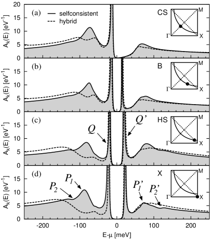
Figure 2: Quasiparticle spectral functions for selected $\bm{k}$-points defined in Ref. Casek:2005:PRB, and shown in the insets as obtained by using the selfconsistent approach (solid lines) and the hybrid approach (dashed lines) for the superconducting state at $T=20\>\mathrm{K}$. Our notation of spectral structures is introduced in panels (c) and (d).

A detailed discussion of the spectral structures obtained at the hybrid level can be found in Ref. Casek:2005:PRB, . Here we concentrate on the comparison between the results of the selfconsistent and the hybrid approach. The positions of the quasiparticle peaks $Q$, $Q^{\prime}$ are identical, which has been achieved by tuning the input BSC gap of the hybrid approach. The maxima $P_{1}$ and $P^{\prime}_{1}$ of the incoherent part in the selfconsistent case are located closer to the quasiparticle peaks and are considerably sharper. This causes the steeper onset and the sharper maximum of $\sigma_{1}$. It can be seen that this maximum simply reflects the maxima of the incoherent part of $A$ - $P_{1}$ and $P^{\prime}_{1}$.

III.2 Vertex corrections

In this section we focus on the central topic of the paper of how the model spectra change when the VC are included.

Figure 3: The spectra of the optical conductivity, the inverse scattering rate, the mass enhancement factor, and the function $W$ calculated with the vertex corrections neglected (NV) and with the vertex corrections included (VC) for the set of input parameters leading to realistic values of $T_{c}$ and $\Delta$. The insets of panel (a) shows the vertically zoomed area near the conductivity maximum and the spectra of $\sigma_{2}$. In panel (d), only the superconducting state spectra are shown. The vertical dashed lines are drawn to guide the eye. A notation of spectral structures is introduced in (b).

Figure 3 shows the optical conductivity and three related quantities: the inverse scattering rate $[1/\tau](\omega)$ and the mass enhancement factor $[m^{*}/m](\omega)$, that are defined by the extended-Drude-model formula

$$\sigma(\omega)=\frac{\epsilon_{0}\omega_{\mathrm{pl}}^{2}}{[1/\tau](\omega)-\mathrm{i}\omega[m^{*}/m](\omega)}\;,$$ (13)

where $\omega_{\rm pl}$ is the plasma frequency, and $W(\omega)=(2\pi)^{-1}\mathrm{d}^{2}[\omega/\tau(\omega)]/\mathrm{d}\omega^{2}$. For the NS of a weakly coupled isotropic electron-phonon system the function $W(\omega)$ is approximately equal to the electron-phonon spectral density Marsiglio:1998:PhysLett ; Schulga:2001:book . The solid and the dashed lines correspond to the SCS at $T=20\>\mathrm{K}$, the dashed-dotted and the dotted lines to the NS at $T=100\>\mathrm{K}$. The solid and the dashed-dotted lines (the dashed and the dotted lines) correspond to the selfconsistent computation with (without) the VC. The values of the dc conductivity $\sigma_{\mathrm{dc}}$, the effective kinetic energy $K$ (multiplied by $d$ to obtain the dimension of energy), the spectral weight at finite frequencies $I_{f}$, and that of the condensate, $I_{c}$, are given in Table 2. The values of $I_{f}$ and $I_{c}$ have been multiplied by $2\hbar^{2}d/\pi e^{2}$ to allow a direct comparison with those of $Kd$.

$g=2\>\mathrm{eV}$        $T_{c}=77\>\mathrm{K}$   $\Delta_{X}=22\>\mathrm{meV}$ ($20\>\mathrm{K}$)
	$T=20\>\mathrm{K}$		$T=100\>\mathrm{K}$
	$Kd=-0.44688\>\mathrm{eV}$		$Kd=-0.44653\>\mathrm{eV}$
	$I_{f}$ [eV]	$I_{c}$ [eV]	$I_{f}$ [eV]	$I_{c}/|K|$ [%]	$\sigma_{\mathrm{dc}}[\Omega^{-1}\mathrm{cm}^{-1}]$
NV	0.27079	0.17609	0.43205	3.2	$1.62\cdot 10^{4}$
VC	0.29752	0.14936	0.44624	0.1	$1.41\cdot 10^{4}$
$g=3\>\mathrm{eV}$        $T_{c}=89\>\mathrm{K}$   $\Delta_{X}=27\>\mathrm{meV}$ ($20\>\mathrm{K}$)
	$T=20\>\mathrm{K}$		$T=100\>\mathrm{K}$
	$Kd=-0.40741\>\mathrm{eV}$		$Kd=-0.40699\>\mathrm{eV}$
	$I_{f}$ [eV]	$I_{c}$ [eV]	$I_{f}$ [eV]	$I_{c}/|K|$ [%]	$\sigma_{\mathrm{dc}}[\Omega^{-1}\mathrm{cm}^{-1}]$
NV	0.28871	0.11870	0.38580	5.2	$8.0\cdot 10^{3}$
VC	0.31312	0.09429	0.40699	0.0	$7.5\cdot 10^{3}$

Table 2: Values of the effective kinetic energy $K$, the spectral weight at finite frequencies $I_{f}$, and the spectral weight of the singular component (condensate) $I_{c}$ computed without vertex corrections (NV) and with the vertex corrections included (VC). The data are presented for two values of the coupling constant $g$, for the superconducting state at $T=20\>\mathrm{K}$ and for the normal state at $T=100\>\mathrm{K}$. For the normal state, the values of the dc conductivity are also given.

We begin our discussion with the NS. It can be seen in Table 2 that in the absence of VC the sum rule $I_{f}\sim K$ (1) is not fulfilled. It means that the conductivity possesses an unphysical singular component with the spectral weight $I_{c}$ determined by Eq. (4). The values of $I_{c}$ of ca $3\%$ (ca $5\%$) of $-K$ for $g=2\>\mathrm{eV}$ ($g=3\>\mathrm{eV}$) are small but significant. The unphysical component manifests itself also in the spectra of related quantities - see the spectra of $\sigma_{2}$ in the inset of Fig. 3 (a), the drop of $1/\tau$ at low frequencies [Fig. 3 (b)], and the corresponding divergence of $m^{*}/m$ [Fig. 3 (c)]. With the VC included the sum rule is satisfied. The spectral weight increase due to the VC [$\Delta I_{f}(\mathrm{VC})$] is equal to $I_{c}$ (within the numerical error related to discrete $\bm{k}$-sampling). Based on the relatively small values of $I_{c}$, the changes of the spectra due to the VC can be expected to be small. Indeed, only a slight decrease of $\sigma_{1}$ in the FIR can be observed in Fig. 3. The dc conductivity also decreases (see Table 2) which is consistent with the results of Monthoux and Pines Monthoux:1994:PRB . This trend, however, is not universal, as will be discussed in Sec. III.2.1.

In the SCS, the VC increase $I_{f}$, which leads to a reduction of $I_{c}$ (see Table 2). This effect is explored in detail in Sec. III.2.2. The real part of the conductivity is affected mainly near then maximum around $800\>\mathrm{cm}^{-1}$: the VC make it slightly sharper. The changes are further amplified in the spectra of related quantities $1/\tau$ and $W$ to be discussed in Sec. III.2.3.

III.2.1 Spectral weight transfer from FIR to MIR

Figure 3(a) shows a decrease of $\sigma_{1}$ in FIR with the incorporation of the VC which seems to be inconsistent with the increase of the finite-frequency spectral weight $I_{f}$. A resolution of this apparent controversy is provided by Fig. 4, which shows the contribution $\Delta\sigma_{1}(\mathrm{VC})$ of the VC to $\sigma_{1}$ in a wide spectral range. It can be seen that $\Delta\sigma_{1}(\mathrm{VC})$ is negative for $\omega<2000\>\mathrm{cm}^{-1}$ but positive for $\omega>2000\>\mathrm{cm}^{-1}$. The magnitude of the contribution of the latter spectral range to $I_{f}$ is larger than that of the former, which leads to the total increase of $I_{f}$, both for the NS and for the SCS. For the SCS, the magnitude of $\Delta\sigma_{1}(\mathrm{VC})$ becomes small as the frequency approaches zero. This is due to the vanishing real part of conductivity in this limit. Figure 4 further demonstrates that the maximum of $\Delta\sigma_{1}(\mathrm{VC})$ shifts towards higher frequencies and becomes broader with increasing weight of the spin fluctuation continuum.

Figure 4: (a) Contribution of the VC to the real part of the normal state conductivity at $T=100\>\mathrm{K}$ for various values of the relative spin-continuum weight $b_{C}$. The low energy parts of the spectra are shown in the inset. (b) The same for the superconducting state at $T=20\>\mathrm{K}$.

In order to explain the behavior displayed in Fig. 4, we use an extension of the formula (12) that applies to the theory involving the VC. In the generalized formula, which has been obtained by manipulations starting from Eq. (10), the integral on the right hand side of Eq. (12) is replaced with a more general convolution of the spectral functions of the form $\int\mathrm{d}E^{\prime}\int\mathrm{d}E^{\prime\prime}A(\bm{k},E^{\prime})A(\bm{k},E^{\prime\prime})\Xi(E^{\prime},E^{\prime\prime},\hbar\omega)$, with the the Matsubara counterpart of the convolution kernel given by

$$\Xi(E^{\prime},E^{\prime\prime},\mathrm{i}\hbar\nu)=\frac{1}{\hbar\beta}\,\mathrm{Im}\sum_{\mathrm{i}E}\frac{\Gamma(\bm{k},\mathrm{i}E,\mathrm{i}\hbar\nu)}{(\mathrm{i}E+\mathrm{i}\hbar\nu-E^{\prime})(\mathrm{i}E-E^{\prime\prime})}\;.$$ (14)

If we use the bare vertex $\Gamma=\partial\varepsilon/\partial k$, we arrive at the relation $\Xi\propto\delta(E^{\prime\prime}+\hbar\omega-E^{\prime})[n_{F}(E^{\prime\prime})-n_{F}(E^{\prime\prime}+\hbar\omega)]$ which, after performing one of the integrations in the convolution, provides exactly the formula (12). In contrast, any kernel $\Xi$ corresponding to a frequency dependent renormalized vertex will be broader than the delta function and will result in a broadening of the conductivity profile.

The effect of the VC on the conductivity can be vaguely viewed as consisting of two ingredients: (a) the increase of the overall spectral weight $I_{f}$ and (b) the broadening of the conductivity profile, which causes a transfer of spectral weight towards higher frequencies. The point (b) accounts for the trends shown in Fig. 4. The change of the dc conductivity is determined by a competition of (a) and (b). For our choice of the input parameters, the VC reduce the dc conductivity, in some cases, however, where $\Delta I_{f}(\mathrm{VC})$ is large, an increase of $\sigma_{\mathrm{dc}}$ may occur. Some examples can be found in Ref. Kontani:2005:condmat, .

The spectral weight redistribution of Fig. 4 is similar to but considerably smaller than the one that could be expected based on the arguments by Millis et alMillis:2005:PRB . Note, however, that the discrepancy between the value of the quasiparticle velocity along the Brillouin zone diagonal resulting from the present computations of $1.1\>\mathrm{eV\AA}$ for $g=2\>\mathrm{eV}$ ($0.75\>\mathrm{eV\AA}$ for $g=3\>\mathrm{eV}$) and the experimental value for YBCO of ca $1.6\>\mathrm{eV\AA}$ Borisenko:2006:PRL is not as dramatic as in Ref. Millis:2005:PRB, .

III.2.2 Effect of the vertex corrections on the spectral weight of the condensate

We have already noted that the VC significantly increase the values of $I_{f}$ and reduce those of $I_{c}$.

Figure 5: (a) The coupling-constant dependence of the effective kinetic energy and of the intraband spectral weight obtained with the vertex corrections neglected (NV) and with the vertex corrections included (VC). (b) The coupling-constant dependence of the ratio of the condensate weight obtained with the vertex corrections included to that obtained using the vertex corrections neglected.

This is further documented in Fig. 5, which shows $I_{f}$ and $I_{c}$ as functions of the coupling constant $g$. For values of $g^{2}$ of $4-10\>\mathrm{eV}^{2}$, leading to reasonable values of $T_{c}$ and $\Delta$, the magnitude of $\Delta I_{f}(\mathrm{VC})$ is about 6% of that of $K$. It can be seen in part (b) that the corresponding change in the condensate weight $I_{c}$ is up to 20%. At low values of $g$, $\Delta I_{f}(\mathrm{VC})$ scales with $g^{2}$. This can be easily interpreted by considering the diagram series for the correlator (10). The contribution of a diagram with $N$ spin-fluctuation lines connecting the quasiparticle lines in the bubble is proportional to $g^{2N}$. In the limit of small $g$, only the lowest-order diagrams ($N=0$ and $N=1$) survive, leading to the observed behavior.

The temperature dependence of the effective kinetic energy $K$ and the band energy $KE=\sum\epsilon_{\bm{k}}n_{\bm{k}\sigma}$ obtained within Eliashberg theory with SF, was already discussed in Ref. Schachinger:2005:PRB, . Our approach yields a similar behavior of the two quantities. The resulting value of $K(\mathrm{NS},T=20\>\mathrm{K})-K(\mathrm{SCS},T=20\>\mathrm{K})$ is also similar to that obtained by Cásek et al. Casek:2005:PRB using the hybrid approach. The analysis published in Ref. Casek:2005:PRB, , however, cannot be easily extended to the present fully-selfconsistent theory. The contribution $\Delta I_{f}(\mathrm{VC})$ of the VC to $I_{f}$ is only weakly temperature dependent above $T_{c}$. Below $T_{c}$, $\Delta I_{f}(\mathrm{VC})$ slightly decreases, exhibits a minimum, and then increases. The low temperature value is somewhat higher than that of the NS.

III.2.3 Spectral structures of $[1/\tau](\omega)$ and $W(\omega)$ for the superconducting state

Having discussed the global trends of the spectral changes due to the VC, we concentrate here on pronounced features in the spectra of $1/\tau$ and $W$. The SCS spectra of $1/\tau$ shown in Fig. 3 exhibit the famous onset starting around the frequency of the resonance mode $\omega_{0}$, becoming steeper around $500\>\mathrm{cm}^{-1}$ (this feature is labeled as $S$), and reaching a sharp maximum around $800\>\mathrm{cm}^{-1}$. Surprisingly, the maximum is followed by a kink labeled as $K$. Note that the spectra are fairly similar to the experimental ones of optimally doped materials Boris:2004:Science ; Marel:2003:Nature ; Timusk:2004:Nature . All these features appear already in the spectra of $\sigma_{1}$, however, they are more pronounced in those of $1/\tau$. The function $W$ is approximately proportional to the second derivative of $1/\tau$ and can thus be expected to possess two maxima corresponding to the structures $S$ and $K$ and a minimum close to the maximum of $1/\tau$. This is indeed the case, as shown in Fig. 3 (d).

The origin of the feature $S$ has been elucidated by Cásek et alCasek:2005:PRB . It is due to the appearance above $\hbar\omega_{0}+\Delta$ of excitations of the nodal region, consisting of a nodal quasiparticle, an antinodal quasiparticle, and the resonance mode. The arguments of Ref. Casek:2005:PRB, , even though formulated at the level of the hybrid approach, remain to be valid also in the context of the present fully selfconsistent theory. As noted for the first time by Carbotte, Schachinger, and Basov Carbotte:1999:Nature , the energy of the relevant maximum in $W$ is close to $\hbar\omega_{0}+\Delta$.

The sharp maximum of $1/\tau$ and the corresponding minimum of $W$ can be shown to result from transitions $P_{1}\rightarrow Q^{\prime}$ and $Q\rightarrow P^{\prime}_{1}$ (see Fig. 2). The energy of the structure is close to $\hbar\omega_{0}+2\Delta$, which can be understood using the arguments presented in Ref. Casek:2005:PRB, . The presence of this characteristic energy scale in the optical spectra of the high-$T_{c}$ cuprates has been for the first time predicted by Abanov, Chubukov, and Schmalian Abanov:2001:PRB . In their work, the corresponding spectral structure is attributed to processes involving a Bogoljubov quasiparticle with energy $\Delta$ and a sharp onset of the incoherent part of $A(\bm{k},E)$ at $\Delta+\hbar\omega_{0}$.

The kink labeled as $K$ can also be interpreted in terms of the quasiparticle spectral functions. Note that the maxima $P_{1}$ and $P^{\prime}_{1}$ in Fig. 2 that are connected to the maximum of $\sigma_{1}$ and the related structures in the spectra of $1/\tau$ and $W$, are followed by shoulder features, labeled as $P_{2}$ and $P^{\prime}_{2}$, on their high-energy sides. They can be expected, based on Eq. (12), to manifest themselves also in the conductivity. Our detailed calculations show that (a) the shoulder features are indeed responsible for the kink $K$ in $1/\tau$ and (b) they can be attributed to excited states involving two magnetic excitations. We recall that the maxima $P_{1}$ and $P^{\prime}_{1}$ correspond to excited states involving one Bogoljubov quasiparticle and just one magnetic excitation. The characteristic energy of the shoulder features is $2\hbar\omega_{0}+\Delta$ and that of the kink $K$ (which can be associated with transitions $P_{2}\rightarrow Q^{\prime}$ and $Q\rightarrow P^{\prime}_{2}$) is $2\hbar\omega_{0}+2\Delta$. Abanov, Chubukov, and Schmalian Abanov:2001:PRB also predicted a structure located at $2\hbar\omega_{0}+2\Delta$. Their interpretation, however, differs from ours. In their theory, the structure is due to transitions between negative- and positive- energy satellites (incoherent components) of $A$.

In order to check the proposed assignment of the spectral structures, we have studied the $\omega_{0}$-dependence of $1/\tau$ and $W$.

Figure 6: The function $W$ for the superconducting state at $T=20\>\mathrm{K}$ obtained with the vertex corrections neglected (NV) and with the vertex corrections included (VC) for three values of the energy of the resonant mode in the spin susceptibility. The vertical lines are located at the characteristic energies of $\hbar\omega_{0}+\Delta$, $\hbar\omega_{0}+2\Delta$, and $2\hbar\omega_{0}+2\Delta$.

Figure 6 shows the spectra of $W$ for three values of the energy of the magnetic mode. It can be seen that the first maximum and the minimum are located close to $\hbar\omega_{0}+\Delta$ and $\hbar\omega_{0}+2\Delta$, respectively, in agreement with the above considerations. The second maximum corresponding to the kink is, in the absence of VC, located somewhat below $2\hbar\omega_{0}+2\Delta$.

Finally, we address the role of the VC. They lead (a) to an increase in the amplitude of the structures of $1/\tau$ and $W$, which is due to the combined effect of the significant decrease of $\sigma_{2}$ [see the inset of Fig. 3 (a)] and a sharpening of the features in $\sigma_{1}$, and (b), to a slight shift of the structures towards lower energies. The shift may be partially caused by a weak attractive interaction between the quasiparticles leading to an excitonic effect.

IV SUMMARY AND CONCLUSIONS

The changes of the infrared conductivity caused by the vertex corrections (VC) are not dramatic, which provides a justification for earlier computations, where these corrections were neglected. Some aspects of the changes, however, appear to be important.
(i) The normal state conductivity computed without the VC does not satisfy the restricted sum rule. The calculated spectral weight at finite frequencies ($I_{f}$) is by a few percent lower than the value dictated by the sum rule. The incorporation of the VC leads to the increase of $I_{f}$, removing this discrepancy.
(ii) The increase of $I_{f}$ is associated with a broadening of $\sigma_{1}$. The far-infrared conductivity (including the dc value) may decrease or increase depending on the magnitude of the change of $I_{f}$ and the degree of the broadening; at high frequencies the conductivity increases. For our values of the input parameters, $\sigma_{1}$ decreases (increases) below (above) ca $2000\>\mathrm{cm}^{-1}$.
(iii) The increase of $I_{f}$ occurs also for the superconducting state. Since the sum of $I_{f}$ and the spectral weight of the superconducting condensate remains constant, this implies a reduction of the latter. For relevant values of the input parameters, the weight of the condensate decreases by 15-20%.
(iv) The VC lead to an amplification of the characteristic features in the superconducting state spectra of the inverse scattering rate $1/\tau$, that have been used to support the spin-fluctuation scenario: the onset of $1/\tau$ around $500\>\mathrm{cm}^{-1}$ becomes steeper and the maximum around $800\>\mathrm{cm}^{-1}$ more pronounced.

In addition to studying the changes brought about by the VC, we have also investigated the role of selfconsistency by comparing the results obtained using the selfconsistent Eliashberg equations with those of the nonselfconsistent hybrid approach (i.e., approximately, the first iteration of the equations). The main results are (a) the hybrid approach considerably overestimates the magnitude of the quasiparticle selfenergy, which leads to lower values of the conductivity in far-infrared, and (b) some spectral features, in particular the sharp maximum in the superconducting state spectra centered at ca $800\>\mathrm{cm}^{-1}$ and the kink at ca $1000\>\mathrm{cm}^{-1}$ appear only at the selfconsistent level. With the aid of the quasiparticle spectral function $A$, we attribute the kink to the onset of transitions involving incoherent satellites of $A$ corresponding to states with doubly excited resonance mode.

The computed spectra are in reasonable agreement with experimental data of optimally doped cuprates, including such details as the shape of the maximum in the inverse scattering rate. In addition, the theory allows one to interpret most of the features of the data in terms of Bogoljubov quasiparticles and magnetic excitations. In the superconducting state, a crucial role is played by the resonance mode. We are not aware of any comparable interpretation in terms of electron-phonon coupling.

References

- (1) S. M. Quinlan, P. J. Hirschfeld, and D. J. Scalapino, Phys. Rev. B 53, 8575 (1996).
- (2) E. Schachinger, J. P. Carbotte, and F. Marsiglio, Phys. Rev. B 56, 2738 (1997).
- (3) D. Munzar, C. Bernhard, and M. Cardona, Physica C 312, 121 (1999).
- (4) J. P. Carbotte, E. Schachinger, and D. N. Basov, Nature (London) 401, 354 (1999).
- (5) A. Abanov, A.V. Chubukov, J. Schmalian, Phys. Rev. B 63, 180510R (2001).
- (6) P. Cásek, C. Bernhard, J. Humlíček, and D. Munzar, Phys. Rev. B 72, 134526 (2005).
- (7) J. Hwang, T. Timusk, E. Schachinger, and J. P. Carbotte Phys. Rev. B 75, 144508 (2007).
- (8) P. Nozieres and D. Pines, The Theory of Quantum Liquids (Perseus Books, Cambridge, Massachusetts, 1999).
- (9) A.J. Millis, H.D. Drew, Phys. Rev. B 67, 214517 (2003).
- (10) A.J. Millis, A. Zimmers, R.P.S.M. Lobo, N. Bontemps, and C.C. Homes Phys. Rev. B 72, 224517 (2005).
- (11) P. Monthoux, D. Pines, Phys. Rev. B 49, 4261 (1994).
- (12) D. Manske, Theory of Unconventional Superconductors (Springer-Verlag, Berlin, 2004).
- (13) H. Kontani, J. Phys. Soc. Jpn. 75, 013703 (2006).
- (14) H. Kontani, cond-mat/0511015 (unpublished).
- (15) L. Benfatto, S.G. Sharapov, N. Andrenacci, and H. Beck, Phys. Rev. B 71, 104511 (2005).
- (16) D.N. Aristov and R. Zeyher, Phys. Rev. B 72, 115118 (2005).
- (17) P. Monthoux and D. Pines, Phys. Rev. B 47, 6069 (1993).
- (18) M. Eschrig and M.R. Norman, Phys. Rev. B 67, 144503 (2003).
- (19) Y. Nambu, Phys. Rev. 117, 648 (1960)
- (20) J.R. Schrieffer, Theory of Superconductivity (Addison-Wesley, Reading, MA, 1988).
- (21) The values of , are close to the LDA results published in O.K. Andersen, A.I. Liechtenstein, O. Jepsen, and F. Paulsen, J. Phys. Chem. Solids 56, 1573 (1995).
- (22) H.F. Fong, P. Bourges, Y. Sidis, L.P. Regnault, J. Bossy, A. Ivanov, D.L. Milius, I.A. Aksay, and B. Keimer, Phys. Rev. B 61 14773 (2000).
- (23) M. Eschrig, M.R. Norman, Phys. Rev. Lett. 89, 277005 (2002)
- (24) H.J. Vidberg and J.W. Serene, J. Low Temp. Phys. 29, 179 (1977).
- (25) A.V. Boris, N.N. Kovaleva, O.V. Dolgov, T. Holden, C.T. Lin, B. Keimer, and C. Bernhard, Science 304, 708 (2004).
- (26) D. van der Marel, H.J.A. Molegraaf, J. Zaanen, Z. Nussinov, F. Carbone, A. Damascelli, H. Eisaki, M. Greven, P.H. Kes, and M. Li, Nature (London) 425, 271 (2003).
- (27) J. Hwang, T. Timusk, and D.G. Gu, Nature (London) 427, 714 (2004).
- (28) F. Marsiglio, T. Startseva, and J. P. Carbotte, Physics Letters A 245, 172 (1998).
- (29) S. V. Schulga, in Material Science, Fundamental Properties and Future Electronic Applications of high-Tc Superconductors, edited by S. L. Drechsler and T. Mischonov (Kluwer Academic, Dordrecht, 2001), pp. 323-360.
- (30) S.V. Borisenko, A.A. Kordyuk, V. Zabolotnyy, J. Geck, D. Inosov, A. Koitzsch, J. Fink, M. Knupfer, B. Büchner, V. Hinkov, C.T. Lin, B. Keimer, T. Wolf, S.G. Chiuzbăian, L. Patthey, and R. Follath, Phys. Rev. Lett. 96 117004 (2006).
- (31) E. Schachinger and J.P. Carbotte, Phys. Rev. B 72, 014535 (2005).