Nonparametric estimation for Lévy processes
from low-frequency observations

Abstract

We suppose that a Lévy process is observed at discrete time points. A rather general construction of minimum-distance estimators is shown to give consistent estimators of the Lévy-Khinchine characteristics as the number of observations tends to infinity, keeping the observation distance fixed. For a specific $C^{2}$-criterion this estimator is rate-optimal. The connection with deconvolution and inverse problems is explained. A key step in the proof is a uniform control on the deviations of the empirical characteristic function on the whole real line.

2000 Mathematics Subject Classification. Primary 62G15; secondary 62M15.
Keywords and Phrases. Lévy-Khinchine characteristics, density estimation, minimum distance estimator, deconvolution.
Short title. Nonparametric estimation for Lévy processes.

1. Introduction

Lévy processes form the fundamental building block for stochastic continuous-time models with jumps. There is an important trend using Lévy models in finance, see CT04, but also many recent models in physics or biology rely on Lévy processes. We consider here the problem of estimating the Lévy-Khintchine characteristics from time-discrete observations of a Lévy process. Since these characteristics involve the Lévy measure (or jump measure) and we do not want to impose a parametric model, we face a nonparametric estimation problem.

When the Lévy process $(X_{t})_{t\geqslant 0}$ is observed at high frequency, at times $(t_{i})_{i=0,\ldots,n}$ with $\max_{i}(t_{i}-t_{i-1})$ small, then a large increment $X_{t_{i}}-X_{t_{i-1}}$ indicates that a jump occurred between time $t_{i-1}$ and $t_{i}$. Based on this insight and the continuous-time observation analogue, nonparametric inference for Lévy processes from high-frequency data has been considered by BB82, FH06 and Nish07. For low-frequency observations, however, we cannot be sure to what extent the increment $X_{t_{i}}-X_{t_{i-1}}$ is due to one or several jumps or just to the Brownian motion part of the Lévy process. The only way to draw inference is to use that the increments form independent realisations of infinitely divisible probability distributions. We shall assume that we dispose of equidistant observations at $t_{i}=i\Delta$, $i=0,\ldots,n$, and consider the asymptotic behaviour of estimators for $n\to\infty$ and $\Delta>0$ fixed. This can be cast into the classical framework of i.i.d. observations $(X_{i\Delta}-X_{(i-1)\Delta})_{i=1,\ldots,n}$ from an infinitely divisible distribution. A natural question in this framework is to estimate the underlying Lévy-Khintchine characteristics. In this general setting we are only aware of the work by WK03 who propose and implement an approach for estimating the jump distribution by a fixed spectral cut-off procedure, which is related to the pilot estimator in Section 5 below. In the special case of compound Poisson processes the problem of estimating the jump density is known as decompounding, see EGS07, Gug07 and the references therein. For parametric inference under the assumption of a stable law see e.g. FM81b. A related low-frequency problem for the canonical function in Lévy-Ornstein-Uhlenbeck processes has been considered by Hol05, where a consistent estimator has been constructed.

In Section 2 we recall basic facts about Lévy processes and prepare the idea of minimum-distance estimators based on the empirical characteristic function. Under very general conditions we then show in Section 3 consistency of these estimators for the Lévy-Khintchine characteristics. The only way to achieve this is to merge the diffusion coefficient $\sigma^{2}$ and the Lévy measure $\nu$ to a single quantity $\nu_{\sigma}$, which is a finite Borel measure, and to consider weak convergence of estimators of $\nu_{\sigma}$. In Section 4 we construct a rate-optimal estimator using a minimum-distance fit, based on a $C^{2}$-criterion for the empirical characteristic function. A fundamental tool is Theorem 4.1, which gives a uniform control on the deviations of the empirical characteristic function on the whole real line and may be of independent interest. The optimal rates of convergence depend on the decay of the characteristic function as in deconvolution problems. Interestingly, our estimator attains the optimal rates without knowing this decay behaviour and without any further regularisation parameter. In Section 5 we briefly discuss the implementation of the estimator, using a two-step procedure, and show a typical numerical example. Most proofs are postponed to Section 6.

2. Basic notions, assumptions, and a few simple facts

We assume that we observe a one-dimensional Lévy process $(X_{t})_{t\geqslant 0}$ at equidistant time points $0=t_{0}<t_{1}<\cdots<t_{n}$. Such a process is characterized by its characteristic function

$$\varphi(u,t;\bar{b},\sigma,\nu)\,:=\,{\mathbb{E}}[\exp(iuX_{t})]\,=\,\exp(t\;\Psi(u;\bar{b},\sigma,\nu)),\qquad u\in{\mathbb{R}},$$

where

$$\Psi(u)\,=\,\Psi(u;\bar{b},\sigma,\nu)\,=\,iu\bar{b}\,-\,\frac{\sigma^{2}}{2}u^{2}\,+\,\int_{{\mathbb{R}}}\left(e^{iux}\,-\,1\,-\,\tfrac{iux}{1+x^{2}}\right)\,\nu(dx).$$

The triplet $(\bar{b},\sigma,\nu)$ is called Lévy-Khintchine characteristic or characteristic triplet with drift-like part $\bar{b}\in{\mathbb{R}}$, volatility $\sigma\geqslant 0$ and jump measure $\nu$, which is a non-negative $\sigma$-finite measure on $({\mathbb{R}},{\mathcal{B}})$ with $\int\frac{x^{2}}{1+x^{2}}\,\nu(dx)<\infty$. The function $\Psi$ is called characteristic exponent or cumulant function.

For reasons explained below, we introduce a measure $\bar{\nu}_{\sigma}$ by

$$\bar{\nu}_{\sigma}(dx)\,=\,\sigma^{2}\delta_{0}(dx)\,+\,\frac{x^{2}}{1+x^{2}}\,\nu(dx),$$

where $\delta_{0}$ denotes the point measure in zero. This gives another representation of $\Psi$ in terms of $\bar{b}\in{\mathbb{R}}$ and the finite Borel measure $\bar{\nu}_{\sigma}$ as

$$\Psi(u)\,=\,\Psi(u;\bar{b},\bar{\nu}_{\sigma})\,=\,iu\bar{b}\,+\,\int_{\mathbb{R}}\frac{(e^{iux}-1)(1+x^{2})-iux}{x^{2}}\,\bar{\nu}_{\sigma}(dx).$$

Here we have used the continuous extension of the integrand at $x=0$, which evaluates to $-u^{2}/2$. Let $P_{\bar{b},\bar{\nu}_{\sigma}}$ denote the probability distribution with characteristic function $\varphi({\scriptstyle\bullet},t;\bar{b},\bar{\nu}_{\sigma})=\exp(t\,\Psi({\scriptstyle\bullet};\bar{b},\bar{\nu}_{\sigma}))$ for some fixed $t>0$. Writing $\mu_{n}\Longrightarrow\mu$ for weak convergence of the finite Borel measures $\mu_{n}$ to the finite Borel measure $\mu$ on $({\mathbb{R}},{\mathcal{B}})$, the following well-known result will be essential in the sequel (Theorem VII.2.9 and Remark VII.2.10 in JS02 or Theorem 19.1 in GK68).

Proposition 2.1.

The convergence $P_{\bar{b}_{n},\bar{\nu}_{\sigma,n}}\Longrightarrow P_{\bar{b},\bar{\nu}_{\sigma}}$ takes place if and only if $\bar{b}_{n}\to\bar{b}$ and $\bar{\nu}_{\sigma,n}\Longrightarrow\bar{\nu}_{\sigma}$.

By the scaling properties of Lévy processes there is no loss in generality when we suppose $t_{k}=k$, $k=0,\ldots,n$. We write $\varphi(u;\bar{b},\bar{\nu}_{\sigma})$ short for $\varphi(u,1;\bar{b},\bar{\nu}_{\sigma})$. Let us introduce the empirical characteristic function of the increments

$$\widehat{\varphi}_{n}(u):=\frac{1}{n}\sum_{t=1}^{n}e^{iu(X_{t}-X_{t-1})},\qquad u\in{\mathbb{R}}.$$

Since these increments are independent and identically distributed it follows from the Glivenko-Cantelli theorem that

(2.1) $$P_{\bar{b},\bar{\nu}_{\sigma}}\left(\widehat{\varphi}_{n}(u)\,\mathop{\longrightarrow}\limits_{n\to\infty}\,\varphi(u;\bar{b},\bar{\nu}_{\sigma})\quad\forall u\in{\mathbb{R}}\right)\,=\,1.$$

We will consider minimum distance fits, that is, we intend to choose $\widehat{\bar{b}}_{n}$ and $\widehat{\bar{\nu}}_{\sigma,n}$ such that, for an appropriate metric $d$,

(2.2) $$d(\widehat{\varphi}_{n},\varphi({\scriptstyle\bullet};\widehat{\bar{b}}_{n},\widehat{\bar{\nu}}_{\sigma,n}))\,=\,\inf_{\tilde{b}\in{\mathbb{R}},\,\tilde{\nu}_{\sigma}\in{\mathcal{M}}({\mathbb{R}})}d(\widehat{\varphi}_{n},\varphi({\scriptstyle\bullet};\widetilde{b},\widetilde{\nu}_{\sigma})).$$

Here ${\mathcal{M}}({\mathbb{R}})$ denotes the space of all finite Borel measures on $({\mathbb{R}},{\mathcal{B}})$. Our basic motivation for this estimation procedure arises from the fact that an exact maximum likelihood estimator is not feasible since there is in general no closed form expression for the probability density of the observations available. Moreover, it is well-known that methods based on the empirical characteristic function can be asymptotically efficient; see FM81a FM81a,FM81b. Since we are not sure that the infimum in (2.2) is always obtained, we take a sequence of positive reals $(\delta_{n})_{n\in{\mathbb{N}}}$ with $\delta_{n}\to 0$ as $n\to\infty$ and choose $\widehat{\bar{b}}_{n}$ and $\widehat{\bar{\nu}}_{\sigma,n}$ such that

(2.3) $$d(\widehat{\varphi}_{n},\varphi({\scriptstyle\bullet};\widehat{\bar{b}}_{n},\widehat{\bar{\nu}}_{\sigma,n}))\,\leqslant\,\inf_{\tilde{b}\in{\mathbb{R}},\,\tilde{\nu}_{\sigma}\in{\mathcal{M}}({\mathbb{R}})}d(\widehat{\varphi}_{n},\varphi({\scriptstyle\bullet};\widetilde{b},\widetilde{\nu}_{\sigma}))\,+\,\delta_{n}.$$

For the metric $d$, we assume that

(2.4) $$\lim_{n\to\infty}d(\widehat{\varphi}_{n},\varphi({\scriptstyle\bullet};\bar{b},\bar{\nu}_{\sigma}))\,=\,0\qquad P_{\bar{b},\bar{\nu}_{\sigma}}\text{-almost surely}$$

and that the following implication holds:

(2.8) $$\left\{\begin{array}[]{ll}&\lim_{n\to\infty}d(\varphi({\scriptstyle\bullet};\bar{b}_{n},\bar{\nu}_{\sigma,n}),\varphi({\scriptstyle\bullet};\bar{b},\bar{\nu}_{\sigma}))\,=\,0\\ \Longrightarrow&\\ &\lim_{n\to\infty}\int_{s}^{t}\varphi(u;\bar{b}_{n},\bar{\nu}_{\sigma,n})\,du\,=\,\int_{s}^{t}\varphi(u;\bar{b},\bar{\nu}_{\sigma})\,du\quad\forall s,t\in{\mathbb{R}}.\end{array}\right.$$

A simple example of such a distance is given by the weighted $L^{p}$-norms,

$$d(\varphi_{1},\varphi_{2})\,=\,\Big{(}\int_{-\infty}^{\infty}|\varphi_{1}(u)-\varphi_{2}(u)|^{p}w(u)\,du\Big{)}^{1/p},$$

where $p\geqslant 1$ and $w:{\mathbb{R}}\rightarrow(0,\infty)$ is a continuous weight function with $\int_{-\infty}^{\infty}w(u)\,du<\infty$. Then Assumption (2.4) follows by dominated convergence from the convergence result (2.1), while Assumption (2.8) is immediate.

3. Consistency

We derive from the triangle inequality, the definition of the minimum-distance estimator and Assumption (2.4) that

$$d(\varphi({\scriptstyle\bullet};\widehat{\bar{b}}_{n},\widehat{\bar{\nu}}_{\sigma,n}),\varphi({\scriptstyle\bullet};\bar{b},\bar{\nu}_{\sigma})) \leqslant d(\varphi({\scriptstyle\bullet};\widehat{\bar{b}}_{n},\widehat{\bar{\nu}}_{\sigma,n}),\widehat{\varphi}_{n})\,+\,d(\widehat{\varphi}_{n},\varphi({\scriptstyle\bullet};\bar{b},\bar{\nu}_{\sigma}))$$

$$\leqslant 2d(\widehat{\varphi}_{n},\varphi({\scriptstyle\bullet};\bar{b},\bar{\nu}_{\sigma}))\,+\,\delta_{n}$$

$$\longrightarrow 0\qquad P_{\bar{b},\bar{\nu}_{\sigma}}\text{-a.s.}$$

By Assumption (2.8) this implies for the integrated characteristic function that

(3.2) $$P_{\bar{b},\bar{\nu}_{\sigma}}\left(\int_{s}^{t}\varphi(u;\widehat{\bar{b}}_{n},\widehat{\bar{\nu}}_{\sigma,n})\,du\,\mathop{\longrightarrow}\limits_{n\to\infty}\,\int_{s}^{t}\varphi(u;\bar{b},\bar{\nu}_{\sigma})\,du\quad\forall s,t\in{\mathbb{R}}\right)\,=\,1.$$

By Theorem 6.3.3 in [page 163]Chu74, we obtain from (3.2) that

$$P_{\widehat{\bar{b}}_{n},\widehat{\bar{\nu}}_{\sigma,n}}\,\longrightarrow_{v}\,P_{\bar{b},\bar{\nu}_{\sigma}}\qquad P_{\bar{b},\bar{\nu}_{\sigma}}\text{-a.s.},$$

where ‘$\longrightarrow_{v}$’ denotes vague convergence to a possibly defective (that is, with a mass less than 1) measure. However, since this vague limit is a probability measure, it turns out that the mode of convergence is actually the weak one, that is,

(3.3) $$P_{\widehat{\bar{b}}_{n},\widehat{\bar{\nu}}_{\sigma,n}}\,\Longrightarrow\,P_{\bar{b},\bar{\nu}_{\sigma}}\qquad P_{\bar{b},\bar{\nu}_{\sigma}}\text{-a.s.}$$

As an immediate consequence of Equation (3.3) and Proposition 2.1 above we obtain the following consistency result for the parameters of the Lévy process:

Theorem 3.1.

If the distance $d$ satisfies properties (2.4) and (2.8), then the minimum distance fit $(\widehat{\bar{b}}_{n},\widehat{\bar{\nu}}_{\sigma,n})$ is a strongly consistent estimator, that is, with probability one we have for $n\to\infty$

$$\widehat{\bar{b}}_{n}\rightarrow\bar{b}\qquad\mbox{ and }\qquad\widehat{\bar{\nu}}_{\sigma,n}\Longrightarrow\bar{\nu}_{\sigma}.$$

Remark 3.2.

Without further assumptions we cannot estimate the diffusion parameter $\sigma$ in a uniformly consistent way. We have for example that the stable law with characteristic function $\varphi_{\alpha}(u)=e^{-\lvert u\rvert^{\alpha}/2}$ converges for $\alpha\uparrow 2$ to the standard normal law ($\alpha=2$) in total variation norm: by Scheffé’s Lemma it suffices to show pointwise convergence of the density functions, which follows from the $L^{1}$-convergence of the characteristic functions. Hence, for $n$ observations no test can separate the hypotheses $H_{0}:\alpha=2$ and $H_{1}:\alpha<2$. Since we have $\sigma=1$ for $\alpha=2$ and $\sigma=0$ for $\alpha<2$, this implies for the estimation problem uniform inconsistency in the following sense:

$$\limsup_{n\to\infty}\inf_{\hat{\sigma}_{n}}\sup_{\bar{b},\,\bar{\nu}_{\sigma}}P_{\bar{b},\bar{\nu}_{\sigma}}(\lvert\widehat{\sigma}_{n}-\sigma\rvert\geqslant 1/2)>0,$$

where the infimum is taken over all estimators based on $n$ observations. Thus, from a statistical perspective the estimation of the volatility $\sigma$ makes no sense, unless we restrict the class of Lévy processes under consideration, e.g. to the finite intensity case as in BR06.

The practical implementation of the minimum distance method raises naturally the question of computational feasibility. It is certainly not possible to compute $\widehat{\bar{\nu}}_{\sigma,n}$ by an optimisation over the full set ${\mathcal{M}}({\mathbb{R}})$. In our simulations, for example, we approximate the measure $\bar{\nu}_{\sigma}$ by measures with step-wise constant densities. To assess the effect of such an approximation, consider a sequence of subsets ${\mathcal{M}}^{(n)}\subseteq{\mathcal{M}}({\mathbb{R}})$ with the density property that there exist measures $\widetilde{\nu}^{(n)}\in{\mathcal{M}}^{(n)}$ with $\widetilde{\nu}^{(n)}\Longrightarrow\bar{\nu}_{\sigma}$, as $n\to\infty$. The definition from (2.3) is now replaced by

$$d(\widehat{\varphi}_{n},\varphi({\scriptstyle\bullet};\widehat{\bar{b}}_{n},\widehat{\bar{\nu}}_{\sigma,n}))\,\leqslant\,\inf_{\tilde{b}\in{\mathbb{R}},\,\tilde{\nu}_{\sigma}\in{\mathcal{M}}^{(n)}}d(\widehat{\varphi}_{n},\varphi({\scriptstyle\bullet};\widetilde{b},\widetilde{\nu}_{\sigma}))\,+\,\delta_{n}.$$

We obtain instead of (3) that

$$d(\varphi({\scriptstyle\bullet};\widehat{\bar{b}}_{n},\widehat{\bar{\nu}}_{\sigma,n}),\varphi({\scriptstyle\bullet};\bar{b},\bar{\nu}_{\sigma})) \leqslant 2d(\widehat{\varphi}_{n},\varphi({\scriptstyle\bullet};\bar{b},\bar{\nu}_{\sigma}))\,+\,\delta_{n}\,+\,d(\varphi({\scriptstyle\bullet};\bar{b},\bar{\nu}_{\sigma}),\varphi({\scriptstyle\bullet};\bar{b},\widetilde{\nu}^{(n)}))$$

$$\longrightarrow 0\qquad P_{\bar{b},\bar{\nu}_{\sigma}}\text{-a.s.}$$

Hence, we obtain in complete analogy to Theorem 3.1 that with probability one for $n\to\infty$

$$\widehat{\bar{b}}_{n}\rightarrow\bar{b}\qquad\mbox{ and }\qquad\widehat{\bar{\nu}}_{\sigma,n}\Longrightarrow\bar{\nu}_{\sigma}.$$

Given the existence of certain moments for $P_{\bar{b},\bar{\nu}_{\sigma}}$, we could also search our minimum-distance estimator in the class of those parameter values that fit the empirical moments. Using a similar error decomposition and the consistency of the empirical moments, this approach will also yield consistent estimators under mild conditions on the distance $d$.

4. A rate-optimal estimator

4.1. The construction

In this section we intend to devise estimators which attain optimal rates of convergence. We henceforth restrict the class of Lévy processes to those with finite second moments. This is equivalent to requiring that the Lévy measure satisfies $\int x^{2}\nu(dx)<\infty$. In this case the following reparametrisation of the characteristic exponent is much more convenient:

$$\Psi(u;b,\sigma,\nu)\,=\,iub\,-\,\frac{\sigma^{2}}{2}u^{2}\,+\,\int_{{\mathbb{R}}}(e^{iux}\,-\,1\,-\,iux)\,\nu(dx),$$

where the parameter $b=\bar{b}+\int_{{\mathbb{R}}}(x-\frac{x}{1+x^{2}})\nu(dx)$ denotes now indeed the mean trend because of ${\mathbb{E}}[X_{1}]=-i\varphi^{\prime}(0)=b$. Let us mention that this is the original Kolmogorov canonical representation of a Lévy process [Kol32], the historial background of which is nicely exposed by MR06. Instead of $\bar{\nu}_{\sigma}$, we consider the finite measure $\nu_{\sigma}$ defined by

$$\nu_{\sigma}(dx)\,=\,\sigma^{2}\delta_{0}(dx)\,+\,x^{2}\,\nu(dx),$$

which allows the nice identity $\operatorname{Var}(X_{1})=-\varphi^{\prime\prime}(0)+\varphi^{\prime}(0)^{2}=\nu_{\sigma}({\mathbb{R}})$. From now on, we shall express the characteristic exponent in terms of $(b,\nu_{\sigma})$:

$$\Psi(u)\,=\,\Psi(u;b,\nu_{\sigma})\,=\,iub\,+\,\int_{\mathbb{R}}\frac{e^{iux}-1-iux}{x^{2}}\,\nu_{\sigma}(dx).$$

While $b$ can be easily estimated by $\frac{1}{n}\sum_{t=1}^{n}(X_{t}-X_{t-1})=X_{n}/n$, the construction of an optimal nonparametric estimator of $\nu_{\sigma}$ requires more work. Before we start with our search for optimal rates of convergence for estimators of $\nu_{\sigma}$, we have to decide about an appropriate metric to measure the deviation of any potential estimator $\widetilde{\nu}_{\sigma,n}$ from its target $\nu_{\sigma}$.

The parameter $\nu_{\sigma}$ lies in the space of finite Borel measures, which is naturally equipped with the total variation norm. As we have seen above in the consistent estimation problem for $\sigma$, this topology is too strong here. Moreover, we are usually not interested in the problem of estimating $\nu_{\sigma}$ itself, but rather in estimating integrals $\int f\,d\nu_{\sigma}$ for certain integrands $f$. In mathematical finance for example, the so-called $\Delta$ in the quadratic hedging approach requires calculating $\int\frac{C(t,S(1+z))-C(t,S)}{Sz}\,\nu_{\sigma}(dz)$, where $C(t,S)$ denotes the option price at time $t$ and $S$ the corresponding stock price, cf. Proposition 10.5 in CT04. This is why we choose to measure the performance of our estimator by metrizing weak convergence with certain classes $F$ of continuous test functions $f$:

$$l(\widetilde{\nu}_{\sigma,n},\nu_{\sigma})\,=\,\sup\left\{\left|\int f\,d\widetilde{\nu}_{\sigma,n}\,-\,\int f\,d\nu_{\sigma}\right|:\;f\in F\right\}.$$

Note that for any class $F$ of uniformly bounded, equicontinuous functions consistency with respect to weak convergence implies $l(\widetilde{\nu}_{\sigma,n},\nu_{\sigma})\to 0$ [Dud89, Cor. 11.3.4]. For instance, the bounded Lipschitz metric is generated by the test functions of Lipschitz norm less than one.

Let us introduce the Fourier transform for functions $f\in L^{1}({\mathbb{R}})$ or measures $\mu\in{\mathcal{M}}({\mathbb{R}})$ by

$${\mathcal{F}}f(u)=\int f(x)e^{iux}dx,\qquad{\mathcal{F}}\mu(u)=\int e^{iux}\mu(dx),\quad u\in{\mathbb{R}}.$$

Note that we have by Parseval’s equality

$$\int f\,d\nu_{\sigma}\,=\,\frac{1}{2\pi}\int_{-\infty}^{\infty}{\mathcal{F}}f(u)\overline{{\mathcal{F}}\nu_{\sigma}(u)}\,du,$$

provided ${\mathcal{F}}f\in L^{1}({\mathbb{R}})$ [Ka76, Theorem VI.2.2]. Estimation of $\nu_{\sigma}$ turns out to be particularly transparent when we employ the fact that

$$\Psi^{\prime\prime}(u)=\frac{d^{2}}{du^{2}}\int\frac{e^{iux}-1-iux}{x^{2}}\,\nu_{\sigma}(dx)=-{\mathcal{F}}\nu_{\sigma}(u),$$

and consequently

(4.1) $${\mathcal{F}}\nu_{\sigma}(u)\,=\,-\frac{d^{2}}{du^{2}}\log(\varphi(u))\,=\,\frac{{\varphi^{\prime}(u)}^{2}}{\varphi(u)^{2}}\,-\,\frac{\varphi^{\prime\prime}(u)}{\varphi(u)}.$$

Recall that $\int x^{2}\nu(dx)<\infty$ implies ${\mathbb{E}}[X_{t}^{2}]<\infty$ and hence $\varphi\in C^{2}$. Moreover, in order to recover $\Psi$ from $\varphi$ we use the distinguished logarithm of the complex-valued function $u\mapsto\varphi(u)$, which is required to ensure $\log(\varphi(0))=0$ and continuity of $u\mapsto\log(\varphi(u))$, cf. CT04. This formula indicates that estimating $\nu_{\sigma}$ is strongly related to estimating $\varphi$ in a $C^{2}$-sense. Before we study rates of convergence, we need to investigate uniform rates of convergence of the empirical characteristic function $\widehat{\varphi}_{n}$ and its derivatives.

4.2. Estimating the characteristic function

For i.i.d. random variables $(Z_{t})_{t\in{\mathbb{N}}}$, denote by

$$C_{n}(u)\,:=\,n^{-1/2}\sum_{t=1}^{n}\left(e^{iuZ_{t}}\,-\,{\mathbb{E}}[e^{iuZ_{1}}]\right)$$

the normalized characteristic function process. Furthermore, denote by $C_{n}^{(k)}$ its $k$th derivative which exists if ${\mathbb{E}}|Z_{1}|^{k}<\infty$. For an appropriate weight function $w:{\mathbb{R}}\longrightarrow[0,\infty)$, we consider

$${\mathbb{E}}\|C_{n}^{(k)}\|_{L_{\infty}(w)}\,:=\,{\mathbb{E}}\sup_{u\in{\mathbb{R}}}\left\{|C_{n}^{(k)}(u)|w(u)\right\}.$$

For every $k\geqslant 0$ we have the following general result.

Theorem 4.1.

Suppose that $(Z_{t})_{t\in{\mathbb{N}}}$ are i.i.d. random variables with ${\mathbb{E}}|Z_{1}|^{2k+\gamma}<\infty$ for some $\gamma>0$ and let the weight function be defined as $w(u)=(\log(e+|u|))^{-1/2-\delta}$ for some $\delta>0$. Then

$$\sup_{n\geqslant 1}{\mathbb{E}}\|C_{n}^{(k)}\|_{L_{\infty}(w)}\,<\,\infty.$$

Its proof is given in Section 6.1. Let us mention that the logarithmic decay of the weight function $w$ is in accordance with the well known result that $\widehat{\varphi}_{n}\to\varphi$ a.s. holds uniformly on intervals $[-T_{n},T_{n}]$ whenever $\log(T_{n})/n\to 0$, cf. Cs83.

4.3. Upper risk bounds

In view of (4.1) and Theorem 4.1, we define our estimators of $b$ and $\nu_{\sigma}$ by a minimum distance fit based on a weighted $C^{2}$-norm. Defining

$$d^{(2)}(\varphi_{1},\varphi_{2})\,:=\,\sum_{k=0}^{2}\|\varphi_{1}^{(k)}\,-\,\varphi_{2}^{(k)}\|_{L^{\infty}(w)},$$

we choose the estimators $\widehat{b}_{n}\in{\mathbb{R}}$ and $\widehat{\nu}_{\sigma,n}\in{\mathcal{M}}({\mathbb{R}})$ such that

(4.2) $$d^{(2)}\left(\varphi({\scriptstyle\bullet};\widehat{b}_{n},\widehat{\nu}_{\sigma,n}),\widehat{\varphi}_{n}\right)\,\leqslant\,\inf_{\tilde{b}\in{\mathbb{R}},\,\tilde{\nu}_{\sigma}\in{\mathcal{M}}({\mathbb{R}})}d^{(2)}\left(\varphi({\scriptstyle\bullet};\widetilde{b},\widetilde{\nu}_{\sigma}),\widehat{\varphi}_{n}\right)\,+\,\delta_{n},$$

where $\delta_{n}\to 0$ as $n\to\infty$. We verify by Theorem 4.1 that $d^{(2)}$ satisfies Assumptions (2.4) and (2.8), hence, Theorem 3.1 gives immediately a consistency result. Moreover, with the choice $\delta_{n}=O(n^{-1/2})$ these estimators will turn out to be rate-optimal.

While $b$ can always be estimated at rate $n^{-1/2}$, rates of convergence of $\int f\,d\widehat{\nu}_{\sigma,n}$ as an estimator of $\int f\,d\nu_{\sigma}$ depend both on the smoothness of $f$ and on the decay of $|\varphi(u)|$ as $|u|\to\infty$. For the function $f$, we will assume that it belongs to the class

$$F_{s}\,:=\,\left\{f:\;\;\int(1+|u|)^{s}|{\mathcal{F}}f(u)|\,du\,\leqslant\,1\right\},$$

for some $s\geqslant 0$. Note that $\int|{\mathcal{F}}f(u)|\,du\leqslant 1$ implies by the Riemann-Lebesgue Lemma that $f$ is continuous with $\|f\|_{\infty}\leqslant 1$. By Fourier theory the condition $f\in F_{s}$ is slightly stronger than requiring $f\in C^{s}$ with $\lVert f\rVert_{C^{s}}\leqslant 1$ for a suitable norming of $C^{s}$. We therefore introduce a loss function for an estimator $\widehat{\mu}$ of the finite measure $\mu$ by

$$\ell_{s}(\widehat{\mu},\mu):=\sup_{f\in F_{s}}\left|\int f\,d\widehat{\mu}\,-\,\int f\,d\mu\right|.$$

Note that by duality the loss $\ell_{s}$ can be interpreted as a negative smoothness norm of order $-s$.

The faster $|\varphi(u)|$ decays, the more difficult it will be to estimate $\nu_{\sigma}$. We consider in particular the following three cases:

• Gaussian part
  If $\sigma^{2}>0$, then the characteristic function $\varphi$ has Gaussian tails, i.e.

  $$\log|\varphi(u)|\,=\,\operatorname{Re}\left(\log\varphi(u)\right)\,=\,-\sigma^{2}u^{2}/2(1\,+\,o(u)),\qquad\mbox{as }|u|\to\infty.$$

  (To see this, note that $F(x,u):=(e^{iux}-1-iux)/(ux)^{2}$ is uniformly bounded with $\lim_{|u|\to\infty}F(x,u)=0$ for $x\neq 0$ such that by dominated convergence $\lim_{|u|\to\infty}\int_{{\mathbb{R}}}F(x,u)x^{2}\,\nu(dx)=0$ and thus $\log\varphi(u)=-\sigma^{2}u^{2}/2+o(u^{2})$.)

• Exponential decay
  Here the characteristic function $\varphi$ decays at most exponentially, i.e. for some $\alpha>0$, $C>0$,

  $$|\varphi(u)|\,\geqslant\,Ce^{-\alpha|u|},\qquad\mbox{for all }u\in{\mathbb{R}}.$$

  Examples of distributions with this property include normal inverse Gaussian [CT04, page 117], and generalized tempered stable distributions [CT04, page 122].

• Polynomial decay
  In this case the characteristic function satisfies, for some $\beta\geqslant 0$, $C>0$,

  $$|\varphi(u)|\,\geqslant\,C(1\,+\,|u|)^{-\beta},\qquad\mbox{for all }u\in{\mathbb{R}}.$$

  Typical examples for this are the compound Poisson distribution, the gamma distribution, the variance gamma distribution and the generalized hyperbolic distribution [CT04, pages 75, 116, 117, 127].

The proof of the following main theorem is postponed to Section 6.2.

Theorem 4.2.

Suppose that ${\mathbb{E}}_{b,\nu_{\sigma}}|X_{1}|^{4+\gamma}<\infty$ for some $\gamma>0$. We choose the weight function $w$ as $w(u)=(\log(e+|u|))^{-1/2-\delta}$, where $\delta$ is any positive number. The estimators $\widehat{b}_{n}$ and $\widehat{\nu}_{\sigma,n}$ of $b$ and $\nu_{\sigma}$, respectively, are chosen according to (4.2) with $\delta_{n}=O(n^{-1/2})$. Then

$${\mathbb{E}}_{b,\nu_{\sigma}}|\widehat{b}_{n}\,-\,b|\,=\,O(n^{-1/2})$$

and for any $s>0$

$$\ell_{s}(\widehat{\nu}_{\sigma,n},\nu_{\sigma})\,=\,O_{P_{b,\nu_{\sigma}}}\left(n^{-1/2}{\scriptstyle\bullet}\sup_{u\in[0,U_{n}]}\left\{\frac{(1+u)^{2-s}}{w(u)|\varphi(u;b,\nu_{\sigma})|}\right\}\right),$$

where

$$U_{n}:=\inf\left\{u>0:\;\frac{(1+u)^{2}n^{-1/2}}{w(u)|\varphi(u;b,\nu_{\sigma})|}\geqslant 1\right\}.$$

The constants in the risk bounds depend continuously on $\lvert b\rvert$ and $\nu_{\sigma}({\mathbb{R}})$. In the specific cases we obtain the following rates of convergence for $\ell_{s}(\widehat{\nu}_{\sigma,n},\nu_{\sigma})$ in $P_{b,\nu_{\sigma}}$-probability:

(a) Gaussian part:

$(\log n)^{-s/2}$

(b) Exponential decay:

$(\log n)^{-s}$

(c) Polynomial decay of order $\beta\geqslant 0$:

$[(\log n)^{1/2+2\delta}n^{-1/2}]^{s/\beta}\vee n^{-1/2}$.

Remark 4.3.

The results are presented for convergence in probability, but the proof immediately yields convergence of moments of order $1/2$ of the loss in cases (a), (b), cf. Equation (6.4). Higher moments are achieved whenever the order of the moment bound in Theorem 4.1 can be increased.

4.4. Lower risk bounds

We prove that the rates of convergence obtained in Theorem 4.2 for cases (a), (b), (c) are optimal, at least up to a logarithmic factor in the latter case. The proof in Section 6.3 can be naturally generalized to cover further decay scenarios of the characteristic function.

Theorem 4.4.

For $C,\bar{C}>0$ large enough and for any $\alpha>0$, $\beta\geqslant 0$ introduce the following nonparametric classes of $\nu_{\sigma}$:

$${\mathcal{A}}(C,\sigma) :=\left\{\nu_{\sigma}\in{\mathcal{M}}({\mathbb{R}})\,\Big{|}\,\nu_{\sigma}({\mathbb{R}})\leqslant C\right\}\text{ ($\sigma>0$),}$$

$${\mathcal{B}}(C,\alpha) :=\left\{\nu_{\sigma}\in{\mathcal{M}}({\mathbb{R}})\,\Big{|}\,\nu_{\sigma}({\mathbb{R}})\leqslant C,\,|\varphi(u)|\geqslant\bar{C}e^{-\alpha\lvert u\rvert}\right\}\text{ ($\sigma=0$),}$$

$${\mathcal{C}}(C,\bar{C},\beta) :=\left\{\nu_{\sigma}\in{\mathcal{M}}({\mathbb{R}})\,\Big{|}\,\nu_{\sigma}({\mathbb{R}})\leqslant C,\,\lvert\varphi(u)\rvert\geqslant\bar{C}^{-1}(1+\lvert u\rvert)^{-\beta}\right\}\text{ ($\sigma=0$)}.$$

Then we obtain for some fixed $b\in{\mathbb{R}}$ and for any $s>0$ the following minimax lower bounds, where $\widetilde{\nu}_{\sigma,n}$ denotes any estimator of $\nu_{\sigma}$ based on $n$ observations:

(a) $$\exists\varepsilon>0: \liminf_{n\to\infty}\inf_{\tilde{\nu}_{\sigma,n}}\sup_{\nu_{\sigma}\in{\mathcal{A}}(C,\sigma)}P_{b,\nu_{\sigma}}\Big{(}(\log n)^{s/2}\ell_{s}(\widetilde{\nu}_{\sigma,n},\nu_{\sigma})>\varepsilon\Big{)}>0,$$

(b) $$\exists\varepsilon>0: \liminf_{n\to\infty}\inf_{\tilde{\nu}_{\sigma,n}}\sup_{\nu_{\sigma}\in{\mathcal{B}}(C,\alpha)}P_{b,\nu_{\sigma}}\Big{(}(\log n)^{s}\ell_{s}(\widetilde{\nu}_{\sigma,n},\nu_{\sigma})>\varepsilon\Big{)}>0,$$

(c) $$\exists\varepsilon>0: \liminf_{n\to\infty}\inf_{\tilde{\nu}_{\sigma,n}}\sup_{\nu_{\sigma}\in{\mathcal{C}}(C,\bar{C},\beta)}P_{b,\nu_{\sigma}}\Big{(}n^{(s/2\beta)\wedge(1/2)}\ell_{s}(\widetilde{\nu}_{\sigma,n},\nu_{\sigma})>\varepsilon\Big{)}>0.$$

4.5. Discussion

The convergence rates for $\widehat{\nu}_{\sigma,n}$ can be understood in analogy with a deconvolution problem where the Fourier transform of the error density decays like the characteristic function $\varphi$ in our case, see e.g. Fan91. The interesting point here is that this decay property is not assumed to be known and depends on the parameters to be estimated. At first sight, it is rather surprising that our minimum distance estimator adapts automatically to the decay of $\varphi$, even for the whole range of loss functions $\ell_{s}$, $s>0$. This is due to the fact that the noise level in the empirical characteristic function $\widehat{\varphi}_{n}$ is of the same size for different frequencies and this is where we fit our estimator. In contrast, when fitting the characteristic exponent $\Psi$, which is more attractive from a computational point of view and for example advocated in Hol05, we face a highly heteroskedastic noise level in $\log(\widehat{\varphi}_{n}(u))$ governed by $\lvert\varphi(u)\rvert^{-1}$ because of $\log(\widehat{\varphi}_{n}(u))-\Psi(u)\approx(\widehat{\varphi}_{n}(u)-\varphi(u))/\varphi(u)$.

Another point of view on our estimation problem is that we want to estimate the linear functional $\int f\,d\nu_{\sigma}$ based on an inverse problem setting for estimating $\nu_{\sigma}$. In an abstract Hilbert scale context, adaptive estimation for this has been considered by GP03 and their rate for the polynomially ill-posed case reads in our notation $(n/\log(n))^{-(r+s)/(2r+2\beta)}\vee n^{-1/2}$, with $r$ the regularity of $\nu_{\sigma}$, $s$ the regularity of $f$ and $\beta$ the degree of ill-posedness. In our case, we measure the regularity $s$ of $f$ in the Fourier domain by an $L^{1}$-criterion such that a dual $L^{\infty}$-criterion for the regularity of $\nu_{\sigma}$ yields $r=0$ because $\lVert{\mathcal{F}}\nu_{\sigma}\rVert_{\infty}$ is finite. Hence, the rate $(n/\log(n))^{-s/2\beta}\vee n^{-1/2}$, up to the logarithmic factor of power $\delta$, obtained in case (c) of Theorem 4.2, confirms this analogy. We suspect that the gap by a logarithmic factor in the polynomial case between our upper and lower bound is mainly due to a suboptimal lower bound, because $\ell_{s}$ can be expressed in the Fourier domain via

$$\ell_{s}(\widehat{\mu},\mu)=\sup_{f\in F_{s}}{\Bigl{\lvert}\int{\mathcal{F}}f(u)\overline{{\mathcal{F}}(\widehat{\mu}-\mu)(u)}\,du\Bigr{\rvert}}=\sup_{u\in{\mathbb{R}}}(1+\lvert u\rvert)^{-s}\lvert{\mathcal{F}}(\widehat{\mu}-\mu)(u)\rvert,$$

giving a supremum-type norm.

It is certainly remarkable that no regularisation parameter is involved in our estimation procedure which becomes more intuitive by noticing that the results of Section 3 imply consistency already for $s=0$. On the other hand, better rates of convergence can be obtained when we restrict the model to measures $\nu_{\sigma}$ which have a regular Lebesgue density $g_{\sigma}$. A natural plug-in approach yields the kernel-type estimator $\widehat{g}_{\sigma,n,h}(x):=K_{h}\ast\widehat{\nu}_{\sigma,n}(x)$, convolving the minimum-distance estimator with a smooth kernel $K_{h}$ of bandwidth $h>0$. Noting that $\int f\widehat{g}_{\sigma,n,h}=\int(f\ast K_{h})\,d\widehat{\nu}_{\sigma,n}$, we infer that the bound on the stochastic error

$${\Bigl{\lvert}\int f(\widehat{g}_{\sigma,n,h}-K_{h}\ast g_{\sigma})\Bigr{\rvert}}={\Bigl{\lvert}\int(f\ast K_{h})d(\widehat{\nu}_{\sigma,n}-\nu_{\sigma})\Bigr{\rvert}}$$

is controlled by the regularity of $f\ast K_{h}$. To be more specific, consider a function $f$ with $\lvert{\mathcal{F}}f(u)\rvert\asymp(1+\lvert u\rvert)^{-s-1}$ (e.g. $f(x)=e^{-\lvert x\rvert}$ with $s=1$), suppose $\sup_{u}(1+\lvert u\rvert)^{r}\lvert{\mathcal{F}}g_{\sigma}(u)\rvert<\infty$ for $r>0$ and assume polynomial decay of order $\beta\geqslant s$ of the characteristic function. Then $\int(1+\lvert u\rvert)^{\beta}\lvert{\mathcal{F}}f(u){\mathcal{F}}K_{h}(u)\rvert\,du\asymp h^{s-\beta}$ holds such that $ch^{-s+\beta}f\ast K_{h}$ lies in $F_{\beta}$, $c>0$ some small constant, and Theorem 4.2 implies that

$${\Bigl{\lvert}\int f(\widehat{g}_{\sigma,n,h}-K_{h}\ast g_{\sigma})\Bigr{\rvert}}\,=\,O_{P}\left(h^{s-\beta}n^{-1/2}(\log n)^{1/2+2\delta}\right).$$

Together with an easy bias estimate of order $h^{s+r}$ this yields for the estimation error $\lvert\int f(\widehat{g}_{\sigma,n,h}-g_{\sigma})\rvert$ up to logarithmic factors the rate $n^{-(r+s)/(2r+2\beta)}$, provided the bandwidth is chosen in an optimal way. We conclude that our results also allow to obtain risk bounds under smoothness restrictions, which are coherent with the abstract results in GP03. The rates should also be compared with the case of continuous-time observations on $[0,T]$, where FH06 obtained the classical nonparametric rate $T^{-r/(2r+1)}$ for estimating $g_{\sigma}$ on a bounded interval.

5. Implementation

Although the main focus of our work is theoretical, we point out how the minimum distance estimator can be implemented and show a numerical example. The main computational problem is that the procedure requires to minimize a nonlinear functional over the space of all finite measures. One possibility is to use a global optimisation procedure, e.g. based on simulated annealing, cf. HY03 for an application to minimum-distance fits based on characteristic functions. Here we shall look for a good preliminary estimator and minimize the $d^{(2)}$-criterion locally around this pilot estimator, which turns out to be more stable in simulations than global optimisation routines.

We use the identification formula (4.1) to build a first-stage plug-in estimator $(\widetilde{b}_{n},\widetilde{\nu}_{\sigma,n})$. While the mean $b$ will be easily estimated by

$$\widetilde{b}_{n}\,:=\,\frac{1}{n}\sum_{t=1}^{n}(X_{t}-X_{t-1})\,=\,X_{n}/n,$$

we have to be more careful with an estimator of $\nu_{\sigma}$. Since ${\mathcal{F}}\nu_{\sigma}(u)=\varphi^{\prime\prime}(u)/\varphi(u)-(\varphi^{\prime}(u)/\varphi(u))^{2}$ one might be tempted to estimate its Fourier transform just by plugging in the empirical characteristic function $\widehat{\varphi}_{n}$ for $\varphi$. It turns out, however, that the occurrence of $\widehat{\varphi}_{n}(u)$ in the denominator might have unfavorable effects, particularly if $|\varphi(u)|$ is small. To get some intuition for a possible remedy, consider the problem of estimating $1/\varphi(u)$. $1/\widehat{\varphi}_{n}(u)$ is certainly a good estimator as long as $|\widehat{\varphi}_{n}(u)|$ is not too small. On the other hand, since the noise level of $\widehat{\varphi}_{n}(u)$ is $O(n^{-1/2})$ we should no longer rely on $1/\widehat{\varphi}_{n}(u)$ if $\widehat{\varphi}_{n}(u)=O(n^{-1/2})$. To take this into account, one can use $\mbox{I1}_{\{\lvert\hat{\varphi}_{n}(u)\rvert\geqslant\kappa n^{-1/2}\}}/\widehat{\varphi}_{n}(u)$ as an estimator for $1/\varphi(u)$ which can be proven to satisfy

$${\mathbb{E}}_{b,\nu_{\sigma}}\left|\frac{\mbox{I1}_{\{\lvert\hat{\varphi}_{n}(u)\rvert\geqslant\kappa n^{-1/2}\}}}{\widehat{\varphi}_{n}(u)}\,-\,\frac{1}{\varphi(u)}\right|^{p}\,=\,O\left(\left(\frac{n^{-1/2}}{|\varphi(u)|^{2}}\wedge\frac{1}{|\varphi(u)|}\right)^{p}\right),$$

for any positive threshold value $\kappa$ and all $p\in{\mathbb{N}}$. This is what we can at best expect from an estimator of $1/\varphi(u)$. Using this idea we define our preliminary estimator of ${\mathcal{F}}\nu_{\sigma}(u)$ by

(5.1) $${\mathcal{F}}\widetilde{\nu}_{\sigma,n}(u)\,:=\,\left(\frac{\widehat{\varphi}_{n}^{\prime\prime}(u)}{\widehat{\varphi}_{n}(u)}\,-\,\left(\frac{\widehat{\varphi}_{n}^{\prime}(u)}{\widehat{\varphi}_{n}(u)}\right)^{2}\right)\mbox{I1}_{\{\lvert\hat{\varphi}_{n}(u)\rvert\geqslant\kappa n^{-1/2}\}},$$

where $\kappa$ is a positive constant. In Section 6.4 below we shall prove the following result.

Proposition 5.1.

We have ${\mathbb{E}}_{b,\nu_{\sigma}}(\tilde{b}_{n}-b)^{2}=O(n^{-1})$ and for $u\in{\mathbb{R}}$

$${\mathbb{E}}_{b,\nu_{\sigma}}\left|{\mathcal{F}}\widetilde{\nu}_{\sigma,n}(u)\,-\,{\mathcal{F}}\nu_{\sigma}(u)\right|\,=\,O\left(\left(\frac{n^{-1/2}}{|\varphi(u)|}\wedge 1\right)\left(1\,+\,|\Psi^{\prime}(u)|^{2}\right)\right).$$

This will give pointwise rates of convergence in a similar fashion as before and serves well as a starting point of a local optimisation routine. Note that this pilot estimator is very easy and fast to implement. Yet, it has certain drawbacks, most importantly ${\mathcal{F}}\widetilde{\nu}_{\sigma,n}$ is usually not positive semidefinite so that $\widetilde{\nu}_{\sigma,n}$ is not necessarily a non-negative measure.

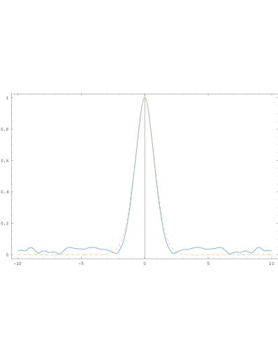
Figure 1. Left: Histogram of the data. Right: modulus of the empirical (solid blue) and true (dashed orange) characteristic function.

In practice, our two-stage procedure works reasonably well. For a numerical example we simulate a Lévy process $(X_{t})_{t\geqslant 0}$ with $\sigma=1$, $b=1$ and $\nu(dx)=x^{-1}e^{-x}\,\mbox{I1}_{\{x>0\}}dx$. The process $X$ is a superposition of an infinite-intensity Gamma process and a standard Brownian motion. The law of its increments $X_{t}-X_{t-1}$ is the convolution of an $N(0,1)$- and an $\operatorname{Exp}(1)$-distribution. We have $n=1000$ observations, see Figure 1(left) for a histogram of the increments. The sample is rather disperse with some increments close to $10$ and a sample mean of $\tilde{b}_{n}=0.936$ (true $b=1$). The true characteristic function has Gaussian decay and its absolute value is shown together with that of the empirical characteristic function in Figure 1(right).

We discretize the pilot estimate $\widetilde{\nu}_{\sigma,n}$ of the jump measure by using a Haar wavelet basis on the interval $[-10,10]$ with 15 basis functions. Moreover, we allow for a point measure in zero to have a better resolution there. Its pilot mass is set to zero. Using the FindMinimum local optimisation procedure in Mathematica, we minimize the $d^{(2)}$-criterion locally around the discretized pilot estimator, constraining to non-negative Lévy measures. In Figure 2(left) we display for the given data the imaginary part of the empirical characteristic function together with the imaginary parts of the other characteristic functions of interest (true, pilot, final estimator). The errors in fitting the real part are less pronounced because there a less oscillations around zero (note $(\operatorname{Re}\varphi)^{\prime}(0)=0$). Typically, the pilot estimator gives already a reasonably good fit and the final estimator has a characteristic function which is closer to the empirical characteristic function than the true one.

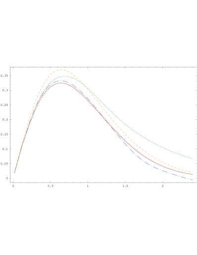
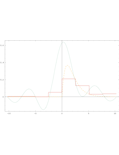
Figure 2. Left: Imaginary part of the empirical (dot-dashed blue), true (orange dashed), pilot (dotted green) and final estimated (red solid) characteristic function. Right: pilot (dotted green), final (red solid) estimator and true (dashed orange) density of $\nu_{\sigma}$; the pilot estimator does not have a point mass in zero.

Figure 2(right) finally shows the densities of the rescaled Lévy measures $\nu_{\sigma}$, but suppresses the point masses in zero. Note that the original Lévy density and also its plug-in estimators have a singularity at zero because of $\nu(dx)=x^{-2}\nu_{\sigma}(dx)$ for $x\not=0$. The parameters are estimated as $\widehat{b}_{n}=0.922$ (true $b=1$) and $\widehat{\nu}_{\sigma,n}(\{0\})^{1/2}=1.092$ (true $\sigma=1$). The pilot estimator has no point mass in zero and its density is therefore large around zero. It is seen that the final estimator improves upon the pilot estimator, in particular by excluding negative values and catching the point mass in zero. Given 1000 observations and a Gaussian deconvolution problem, the estimation problem is quite hard. The rough, step-wise form of the final estimator is not so pleasant for the human eye, but we only want to use this estimator as an integrator of smooth functions and, as discussed above, we could apply a kernel to obtain a smooth density function. As an example for a functional to be estimated, we calculated $\int_{1}^{\infty}x^{-2}\widehat{\nu}_{\sigma}(dx)$ which estimates $\nu([1,\infty))$, the probability of jumps larger than one. In this sample, the true value 0.22 was estimated by 0.16. Let us remark that the high-frequency estimator, using the relative frequency of increments $X_{t}-X_{t-1}$ that are larger than one, yields the estimate 0.46. The large error of the latter confirms a strong violation of the underlying high-frequency assumption that between two observations very rarely more than one larger jump occurs and that the diffusion part is negligible. Hence, the frequency of the observations must indeed be considered as low for the construction of the estimator.

6. Proofs

6.1. Proof of Theorem 4.1

We begin the proof with a few definitions. Given two functions $l,u:{\mathbb{R}}\longrightarrow{\mathbb{R}}$ the bracket $[l,u]$ denotes the set of functions $f$ with $l\leqslant f\leqslant u$. For a set $G$ of functions the $L^{2}$-bracketing number $N_{[\,]}(\varepsilon,G)$ is the minimum number of brackets $[l_{i},u_{i}]$, satisfying ${\mathbb{E}}[(u_{i}(Z_{1})\,-\,l_{i}(Z_{1}))^{2}]\leqslant\varepsilon^{2}$, that are needed to cover $G$. The associated bracketing integral is defined as

$$J_{[\,]}(\delta,G)\,=\,\int_{0}^{\delta}\sqrt{\log(N_{[\,]}(\varepsilon,G))}\,d\varepsilon.$$

Furthermore, a function $\overline{f}$ is called envelope function for $G$, if $|f|\leqslant\overline{f}$ holds for all $f\in G$.

To apply Corollary 19.35 from vdV98, we decompose $C_{n}$ in its real and imaginary parts,

$$\operatorname{Re}(C_{n}(u)) = n^{-1/2}\sum_{t=1}^{n}\left(\cos(uZ_{t})\,-\,{\mathbb{E}}\cos(uZ_{1})\right),$$

$$\operatorname{Im}(C_{n}(u)) = n^{-1/2}\sum_{t=1}^{n}\left(\sin(uZ_{t})\,-\,{\mathbb{E}}\sin(uZ_{1})\right).$$

Accordingly, we consider the following class of functions:

$$G_{k}\,=\,\left\{\left.z\mapsto w(u)\tfrac{\partial^{k}}{\partial u^{k}}\cos(uz)\right|u\in{\mathbb{R}}\right\}\cup\left\{\left.z\mapsto w(u)\tfrac{\partial^{k}}{\partial u^{k}}\sin(uz)\right|u\in{\mathbb{R}}\right\}.$$

An envelope function $\overline{f}_{k}$ for $G_{k}$ is given by $\overline{f}_{k}=|x|^{k}$. Now we obtain from Corollary 19.35 in vdV98 that

(6.1) $${\mathbb{E}}\|C_{n}^{(k)}\|_{L_{\infty}(w)}\,\leqslant\,C\left\{{\mathbb{E}}(\overline{f}_{k}(Z_{1}))^{2}\,+\,J_{[\,]}(\sqrt{{\mathbb{E}}Z_{1}^{2k}},G_{k})\right\}.$$

Since ${\mathbb{E}}Z_{1}^{2k}<\infty$ it remains to bound the bracketing integral on the right-hand side of (6.1). Inspired by Yuk85, we proceed by setting, for every $\varepsilon>0$,

$$M\,:=\,M(\varepsilon,k)\,:=\,\inf\left\{m>0\mid{\mathbb{E}}[Z_{1}^{2k}\,\mbox{I1}_{\{|Z_{1}|>m\}}]\leqslant\varepsilon^{2}\right\}.$$

Furthermore, we set, for grid points $u_{j}\in{\mathbb{R}}$ to be specified below,

$$g_{j}^{\pm}(z) =\left(w(u_{j})\tfrac{\partial^{k}}{\partial u^{k}}\cos(u_{j}z)\pm\varepsilon|z|^{k}\right)\mbox{I1}_{[-M,M]}(z)\,\pm\,\|w\|_{\infty}|z|^{k}\,\mbox{I1}_{[-M,M]^{c}}(z),$$

$$h_{j}^{\pm}(z) =\left(w(u_{j})\tfrac{\partial^{k}}{\partial u^{k}}\sin(u_{j}z)\pm\varepsilon|z|^{k}\right)\mbox{I1}_{[-M,M]}(z)\,\pm\,\|w\|_{\infty}|z|^{k}\,\mbox{I1}_{[-M,M]^{c}}(z).$$

We obtain for the width of the brackets that

$${\mathbb{E}}\left[\left(g_{j}^{+}(Z_{1})\,-\,g_{j}^{-}(Z_{1})\right)^{2}\right] \leqslant{\mathbb{E}}\left[4\varepsilon^{2}Z_{1}^{2k}\,\mbox{I1}_{[-M,M]}(Z_{1})\,+\,4\|w\|_{\infty}^{2}Z_{1}^{2k}\mbox{I1}_{[-M,M]^{c}}(Z_{1})\right]$$

$$\leqslant 4\varepsilon^{2}\left({\mathbb{E}}Z_{1}^{2k}\,+\,\|w\|_{\infty}^{2}\right),$$

and, analogously,

$${\mathbb{E}}\left[\left(h_{j}^{+}(Z_{1})\,-\,h_{j}^{-}(Z_{1})\right)^{2}\right]\,\leqslant\,4\varepsilon^{2}\left({\mathbb{E}}Z_{1}^{2k}\,+\,\|w\|_{\infty}^{2}\right).$$

It remains to choose the grid points $u_{j}$ in such a way that the brackets cover the set $G_{k}$. We consider an arbitrary $u\in{\mathbb{R}}$ and any grid point $u_{j}$. Then with the Lipschitz constant $\mbox{\rm Lip}(w)$ of the weight function $w$

$$\left|w(u)\tfrac{\partial^{k}}{\partial u^{k}}\cos(uz)\,-\,w(u_{j})\tfrac{\partial^{k}}{\partial u^{k}}\cos(u_{j}z)\right|$$

$$\leqslant |z|^{k}\min\{|u-u_{j}|(\mbox{\rm Lip}(w)\,+\,\|w\|_{\infty}|z|),w(u)\,+\,w(u_{j})\}.$$

Therefore, the function $z\mapsto w(u)\tfrac{\partial^{k}}{\partial u^{k}}\cos(uz)$ is contained in the bracket $[g_{j}^{-},g_{j}^{+}]$ if

$$\min\{|u-u_{j}|(\mbox{\rm Lip}(w)\,+\,\|w\|_{\infty}M),w(u)\,+\,w(u_{j})\}\,\leqslant\,\varepsilon.$$

Consequently, we choose the grid points as

$$u_{j}\,=\,j\varepsilon/(\mbox{\rm Lip}(w)\,+\,\|w\|_{\infty}M(\varepsilon,k)),$$

for $|j|\leqslant J(\varepsilon)$, where $J(\varepsilon)$ is the smallest integer such that $u_{J(\varepsilon)}$ is greater than or equal to

$$U(\varepsilon)\,=\,\inf\left\{u>0\mid\sup_{v:\,|v|\geqslant u}w(v)\leqslant\varepsilon/2\right\}.$$

This yields the estimate $N_{[\,]}(\varepsilon,G_{k})\,\leqslant\,2(2J(\varepsilon)\,+\,1)$. It follows from the generalized Markov inequality that

$$M(\varepsilon,k)\,\leqslant\,\left({\mathbb{E}}[|Z_{1}|^{2k+\gamma}]/\varepsilon^{2}\right)^{1/\gamma}.$$

Now we obtain from the inequality

$$J(\varepsilon)\,\leqslant\,2U(\varepsilon)(\mbox{\rm Lip}(w)\,+\,\|w\|_{\infty}M(\varepsilon,k))/\varepsilon\,+\,1$$

that $\log(N_{[\,]}(\varepsilon,G_{k}))=O(\log(J(\varepsilon)))=O(\varepsilon^{-(\delta+1/2)^{-1}}+\log(\varepsilon^{-1-2/\gamma}))=O(\varepsilon^{-\kappa})$ for $\kappa=(\delta+1/2)^{-1}<2$. This implies

$$\int_{0}^{\delta}\sqrt{\log(N_{[\,]}(\varepsilon,G_{k}))}\,d\varepsilon\,<\,\infty,$$

as required. ∎

6.2. Proof of Theorem 4.2

To simplify the notation, we use the abbreviations $\Psi_{n}(u)=\Psi(u;\widehat{b}_{n},\widehat{\nu}_{\sigma,n})$ and $\varphi_{n}(u)=\exp(\Psi_{n}(u))$.

First of all, we obtain from the triangle inequality that

(6.2) $$d^{(2)}(\varphi_{n},\varphi) \leqslant d^{(2)}(\widehat{\varphi}_{n},\varphi)\,+\,d^{(2)}(\widehat{\varphi}_{n},\varphi_{n})$$

$$\leqslant 2d^{(2)}(\widehat{\varphi}_{n},\varphi)\,+\,\delta_{n}.$$

Proof for $\widehat{b}_{n}$

We have that $\varphi^{\prime}(0)=ib$ and $\varphi_{n}^{\prime}(0)=i\widehat{b}_{n}$. Therefore, we obtain from (6.2) and Theorem 4.1 that

$${\mathbb{E}}_{b,\nu_{\sigma}}|\widehat{b}_{n}\,-\,b| ={\mathbb{E}}_{b,\nu_{\sigma}}|\varphi_{n}^{\prime}(0)\,-\,\varphi^{\prime}(0)|$$

$$\leqslant{\mathbb{E}}_{b,\nu_{\sigma}}d^{(2)}(\varphi_{n},\varphi)$$

$$\leqslant 2{\mathbb{E}}_{b,\nu_{\sigma}}d^{(2)}(\widehat{\varphi}_{n},\varphi)\,+\,\delta_{n}\,=\,O(n^{-1/2}).$$

Proof for $\widehat{\nu}_{\sigma,n}$

We consider the following set of “unfavorable” events:

$$A_{n}\,:=\,\left\{\widehat{\nu}_{\sigma,n}({\mathbb{R}})\,>\,\nu_{\sigma}({\mathbb{R}})\,+\,1\right\}\cup\left\{|\widehat{b}_{n}|\,>\,|b|\,+\,1\right\}.$$

From $\varphi^{\prime}(0)^{2}-\varphi^{\prime\prime}(0)=\nu_{\sigma}({\mathbb{R}})$ and the analogous formula for $\varphi_{n}$ it follows that

$$\lvert\widehat{\nu}_{\sigma,n}({\mathbb{R}})-\nu_{\sigma}({\mathbb{R}})\rvert =\lvert(\varphi^{\prime}(0)^{2}-\varphi_{n}^{\prime}(0)^{2})-(\varphi^{\prime\prime}(0)-\varphi_{n}^{\prime\prime}(0))\rvert$$

(6.3) $$\leqslant(2\lvert\varphi^{\prime}(0)\rvert+d^{(2)}(\varphi,\varphi_{n})+1)d^{(2)}(\varphi,\varphi_{n}),$$

Consequently, the (generalized) Markov inequality yields

$$P_{b,\nu_{\sigma}}(A_{n}) \leqslant {\mathbb{E}}_{b,\nu_{\sigma}}[|\widehat{\nu}_{\sigma,n}({\mathbb{R}})\,-\,\nu_{\sigma}({\mathbb{R}})|\wedge 1]\,+\,{\mathbb{E}}_{b,\nu_{\sigma}}[|\widehat{b}_{n}\,-\,b|]$$

$$\leqslant {\mathbb{E}}_{b,\nu_{\sigma}}\left[\left(\left(2\lvert b\rvert+d^{(2)}(\varphi,\varphi_{n})+1\right)d^{(2)}(\varphi,\varphi_{n})\right)\wedge 1\right]\,+\,{\mathbb{E}}_{b,\nu_{\sigma}}\left[d^{(2)}(\varphi,\varphi_{n})\right]$$

$$\leqslant {\mathbb{E}}_{b,\nu_{\sigma}}\left[(4\lvert b\rvert+2)d^{(2)}(\varphi,\varphi_{n})\right]\,+\,{\mathbb{E}}_{b,\nu_{\sigma}}\left[d^{(2)}(\varphi,\varphi_{n})\right]$$

$$\leqslant (4\lvert b\rvert+3)\left({\mathbb{E}}_{b,\nu_{\sigma}}[d^{(2)}(\widehat{\varphi}_{n},\varphi)]\,+\,\delta_{n}\right)\,=\,O(n^{-1/2}),$$

which implies that

(6.4) $$\mbox{I1}_{A_{n}}{\scriptstyle\bullet}\sup_{f\in{F}_{s}}\left|\int f\,d\widehat{\nu}_{\sigma,n}\,-\,\int f\,d\nu_{\sigma}\right|$$

$$\leqslant \mbox{I1}_{A_{n}}{\scriptstyle\bullet}\sup_{f\in{F}_{s}}\|f\|_{\infty}{\scriptstyle\bullet}\left(\widehat{\nu}_{\sigma,n}({\mathbb{R}})\,+\,\nu_{\sigma}({\mathbb{R}})\right)$$

$$\leqslant 2\;\nu_{\sigma}({\mathbb{R}})\;\mbox{I1}_{A_{n}}\,+\,(2\lvert\varphi^{\prime}(0)\rvert+d^{(2)}(\varphi,\varphi_{n})+1)d^{(2)}(\varphi,\varphi_{n})$$

$$= O_{P_{b,\nu_{\sigma}}}(n^{-1/2}).$$

It remains to analyse the loss under $A_{n}^{c}$. It follows from Parseval’s identity that

(6.5) $$\left|\int f\,d\widehat{\nu}_{\sigma,n}\,-\,\int f\,d\nu_{\sigma}\right|$$

$$= \frac{1}{2\pi}\int_{-\infty}^{\infty}{\mathcal{F}}f(u)\overline{({\mathcal{F}}\widehat{\nu}_{\sigma,n}(u)\,-\,{\mathcal{F}}\nu_{\sigma}(u))}\,du$$

$$= \frac{1}{2\pi}\int_{-\infty}^{\infty}{\mathcal{F}}f(u)\overline{\left\{\left(\big{(}\frac{\varphi_{n}^{\prime}(u)}{\varphi_{n}(u)}\big{)}^{2}\,-\,\big{(}\frac{\varphi^{\prime}(u)}{\varphi(u)}\big{)}^{2}\right)\;-\;\left(\frac{\varphi_{n}^{{}^{\prime\prime}}(u)}{\varphi_{n}(u)}\,-\,\frac{\varphi^{{}^{\prime\prime}}(u)}{\varphi(u)}\right)\right\}}\,du.\quad$$

The differences occurring in the integrand on the right-hand side of (6.5) can be estimated using $\varphi^{\prime}/\varphi=\Psi^{\prime}$, $\varphi_{n}^{\prime}/\varphi_{n}=\Psi_{n}^{\prime}$:

$$\left|\left(\frac{\varphi_{n}^{\prime}(u)}{\varphi_{n}(u)}\right)^{2}\,-\,\left(\frac{\varphi^{\prime}(u)}{\varphi(u)}\right)^{2}\right|=\left|\frac{\varphi_{n}^{\prime}(u)}{\varphi_{n}(u)}\,-\,\frac{\varphi^{\prime}(u)}{\varphi(u)}\right|\;|\Psi_{n}^{\prime}(u)\,+\,\Psi^{\prime}(u)|$$

(6.6) $$\qquad\qquad\qquad\qquad\leqslant\left\{\left|\frac{\varphi_{n}(u)\,-\,\varphi(u)}{\varphi(u)}\right||\Psi_{n}^{\prime}(u)|\,+\,\left|\frac{\varphi_{n}^{\prime}(u)\,-\,\varphi^{\prime}(u)}{\varphi(u)}\right|\right\}\;|\Psi_{n}^{\prime}(u)\,+\,\Psi^{\prime}(u)|$$

and

(6.7) $$\left|\frac{\varphi_{n}^{\prime\prime}(u)}{\varphi_{n}(u)}\,-\,\frac{\varphi^{\prime\prime}(u)}{\varphi(u)}\right| \leqslant \left|\frac{\varphi_{n}(u)\,-\,\varphi(u)}{\varphi(u)}\right|\;\left|\frac{\varphi_{n}^{\prime\prime}(u)}{\varphi_{n}(u)}\right|\,+\,\left|\frac{\varphi_{n}^{\prime\prime}(u)\,-\,\varphi^{\prime\prime}(u)}{\varphi(u)}\right|$$

$$= \left|\frac{\varphi_{n}(u)\,-\,\varphi(u)}{\varphi(u)}\right|\;\left|\Psi_{n}^{\prime\prime}(u)\,+\,\left(\Psi_{n}^{\prime}(u)\right)^{2}\right|\,+\,\left|\frac{\varphi_{n}^{\prime\prime}(u)\,-\,\varphi^{\prime\prime}(u)}{\varphi(u)}\right|.$$

Note that the following estimates hold true under $A_{n}^{c}$:

(6.8) $$|\Psi_{n}^{\prime}(u)| \leqslant |\widehat{b}_{n}|\,+\,|u|\widehat{\nu}_{\sigma,n}({\mathbb{R}})\,\leqslant\,|b|\,+\,1\,+\,|u|(\nu_{\sigma}({\mathbb{R}})\,+\,1),$$

(6.9) $$|\Psi_{n}^{\prime\prime}(u)| \leqslant |{\mathcal{F}}\widehat{\nu}_{\sigma,n}(u)|\,\leqslant\,\widehat{\nu}_{\sigma,n}({\mathbb{R}})\,\leqslant\,\nu_{\sigma}({\mathbb{R}})\,+\,1.$$

Hence, we obtain from (6.5) to (6.9) and the trivial estimate $|{\mathcal{F}}\widehat{\nu}_{\sigma,n}(u)\,-\,{\mathcal{F}}\nu_{\sigma}(u)|\leqslant\widehat{\nu}_{\sigma,n}({\mathbb{R}})\,+\,\nu_{\sigma}({\mathbb{R}})$ that under $A_{n}^{c}$, with some constant $C>0$,

$$\left|\int f\,d\widehat{\nu}_{\sigma,n}\,-\,\int f\,d\nu_{\sigma}\right|$$

$$\leqslant C\;\int_{-\infty}^{\infty}|{\mathcal{F}}f(u)|\;\left(\frac{|\varphi_{n}(u)-\varphi(u)|\,+\,|\varphi_{n}^{\prime}(u)-\varphi^{\prime}(u)|\,+\,|\varphi_{n}^{\prime\prime}(u)-\varphi^{\prime\prime}(u)|}{|\varphi(u)|}(1\,+\,|u|)^{2}\;\wedge\;1\right)\,du$$

$$\leqslant C\;\int_{-\infty}^{\infty}(1\,+\,|u|)^{s}|{\mathcal{F}}f(u)|\,du\;{\scriptstyle\bullet}\;\sup_{u\in{\mathbb{R}}}\left\{(1\,+\,|u|)^{-s}\left(\frac{(1\,+\,|u|)^{2}\;d^{(2)}(\varphi_{n},\varphi)}{w(u)|\varphi(u)|}\;\wedge\;1\right)\right\}$$

$$\leqslant C\;\sup_{u\geqslant 0}\left\{(1\,+\,u)^{-s}\left(\frac{(1\,+\,u)^{2}\;n^{-1/2}}{w(u)|\varphi(u)|}\;\wedge\;1\right)\right\}\;\left(n^{1/2}d^{(2)}(\varphi_{n},\varphi)\,+\,1\right).$$

By monotonicity of $(1+u)^{-s}$ we can replace the supremum over $[0,\infty)$ by the supremum over $[0,U_{n}]$ and we arrive at

(6.10) $${\mathbb{E}}_{b,\nu_{\sigma}}\left[\mbox{I1}_{A_{n}^{c}}{\scriptstyle\bullet}\sup_{f\in F_{s}}\left|\int f\,d\widehat{\nu}_{\sigma,n}\,-\,\int f\,d\nu_{\sigma}\right|\right]$$

$$= O\left(\sup_{u\in[0,U_{n}]}\left\{(1\,+\,u)^{-s}\left(\frac{(1\,+\,u)^{2}n^{-1/2}}{w(u)|\varphi(u)|}\wedge 1\right)\right\}\right).$$

Together with the bound (6.4) on the set $A_{n}$ this yields the asserted general estimate. Tracing back the constants, we see that they depend continuously on $\lvert b\rvert$ and $\nu_{\sigma}({\mathbb{R}})$.

Proof of the rate results (a), (b)

(a) Under the condition $\log|\varphi(u)|=-\sigma^{2}u^{2}/2(1+o(u))$ we have $U_{n}\asymp\sqrt{\log n}$ and we obtain the rate $U_{n}^{-s}=(\log n)^{-s/2}$.

(b) If $|\varphi(u)|\geqslant Ce^{-\alpha u}$, then we have $U_{n}\asymp\log n$ and we obtain the rate $U_{n}^{-s}=(\log n)^{-s}$.

Proof of the rate result (c)

The same reasoning as for cases (a) and (b) would only yield the rate $((\log n)^{1/2+\delta}n^{1/2})^{-s/(\beta+2)}$ for $s\in(0,\beta+2]$ and the parametric rate for $s>\beta+2$. In the polynomial case (c), though, better estimates for $\lvert\Psi_{n}^{\prime}(u)\rvert$ hold, i.e. we can improve upon (6.8). First, we formulate and prove a lemma for $\lvert\Psi^{\prime}(u)\rvert$.

Lemma 6.1.

If a Lévy process with a finite first moment has a characteristic function (at time $t=1$) satisfying $|\varphi(u)|\,\geqslant\,C(1\,+\,|u|)^{-\beta}$ for some $\beta\geqslant 0$, $C>0$ and all $u\in{\mathbb{R}}$, then $\int_{[-1,+1]}\lvert x\rvert^{\alpha}\nu(dx)$ is finite for all $\alpha>0$ and the derivative of its characteristic exponent is uniformly bounded:

$$\sup_{u\in{\mathbb{R}}}\lvert\Psi^{\prime}(u)\rvert<\infty.$$

Proof of Lemma 6.1.

Since we have necessarily $\sigma^{2}=0$ in the Lévy-Khinchine characteristic as well as $\int_{[-1,1]^{c}}|x|\,\nu(dx)<\infty$ from the first moment condition, the additional property $\int_{[-1,+1]}\lvert x\rvert\nu(dx)<\infty$ implies

$$\sup_{u\in{\mathbb{R}}}\lvert\Psi^{\prime}(u)\rvert\,=\,\sup_{u\in{\mathbb{R}}}{\Bigl{\lvert}ib+\int(e^{iux}-1)ix\,\nu(dx)\Bigr{\rvert}}\,\leqslant\,\lvert b\rvert+2\int\lvert x\rvert\,\nu(dx)\,<\,\infty.$$

It therefore remains to prove the first result for any $\alpha>0$. We obtain with $c:=\min_{u\in[1,2]}(1-\cos(u))>0$:

$$\int_{[-1,+1]}\lvert x\rvert^{\alpha}\nu(dx) \leqslant\sum_{n=1}^{\infty}\int_{\{x:\,2^{-n}\leqslant\lvert x\rvert\leqslant 2^{-n+1}\}}\lvert x\rvert^{\alpha}\nu(dx)$$

$$\leqslant\sum_{n=1}^{\infty}2^{-\alpha(n-1)}\int_{\{x:\,2^{-n}\leqslant\lvert x\rvert\leqslant 2^{-n+1}\}}c^{-1}(1-\cos(2^{n}x))\,\nu(dx)$$

$$\leqslant c^{-1}\sum_{n=1}^{\infty}2^{-\alpha(n-1)}\operatorname{Re}(-\Psi(2^{n}))$$

$$\leqslant c^{-1}\sum_{n=1}^{\infty}2^{-\alpha(n-1)}\left(\log(C^{-1})+\beta\log(1\,+\,2^{n})\right).$$

This latter series is obviously finite. ∎

Resuming the proof for case (c), we remark that $\lvert\varphi(u)\rvert\geqslant C(1+\lvert u\rvert)^{-\beta}$ implies for any $U>0$

$$P_{b,\nu_{\sigma}} \left(\exists u\in[-U,U]:\>\lvert\varphi_{n}(u)\rvert<\frac{C}{2}(1\,+\,|u|)^{-\beta}\right)$$

$$\leqslant P_{b,\nu_{\sigma}}\left(\sup_{\lvert u\rvert\leqslant U}\lvert\varphi_{n}(u)-\varphi(u)\rvert(1+\lvert u\rvert)^{\beta}\geqslant C/2\right)$$

$$\leqslant\frac{2}{C}{\mathbb{E}}[\lVert\varphi_{n}-\varphi\rVert_{L^{\infty}(w)}]w(U)^{-1}(1+U)^{\beta}=O(n^{-1/2}w(U)^{-1}(1+U)^{\beta}).$$

Consequently, for $U_{n}\to\infty$ with $w(U_{n})^{-1}U_{n}^{\beta}=o(n^{1/2})$ we have

(6.11) $$\lim_{n\to\infty}P_{b,\nu_{\sigma}}\left(\forall u\in[-U_{n},U_{n}]:\>\lvert\varphi_{n}(u)\rvert\geqslant\frac{C}{2}(1\,+\,|u|)^{-\beta}\right)=1;$$

in the sequel we shall work with $U_{n}=n^{1/(2\beta)}(\log n)^{-(1/2+2\delta)/\beta}$. Theorem 4.1, Lemma 6.1 and Equation (6.11) then yield

(6.12) $$\sup_{\lvert u\rvert\leqslant U_{n}}|\Psi_{n}^{\prime}(u)-\Psi^{\prime}(u)| \leqslant \sup_{\lvert u\rvert\leqslant U_{n}}\left\{\frac{|\varphi_{n}^{\prime}(u)-\varphi^{\prime}(u)|}{|\varphi_{n}(u)|}+|\Psi^{\prime}(u)|\frac{|\varphi(u)-\varphi_{n}(u)|}{|\varphi_{n}(u)|}\right\}$$

$$= O_{P}(n^{-1/2})w(U_{n})^{-1}\frac{2}{C}(1+|U_{n}|)^{\beta}.$$

Together with Estimate (6.12) and again Lemma 6.1 we have thus established for $n\to\infty$

(6.13) $$\sup_{\lvert u\rvert\leqslant U_{n}}\lvert\Psi_{n}^{\prime}(u)\rvert\,=\,O_{P}\left(1\,+\,n^{-1/2}w(U_{n})^{-1}|U_{n}|^{\beta}\right)\,=\,O_{P}(1).$$

We therefore get instead of (6.2) the estimate

$$\sup_{f\in F_{s}}\left|\int f\,d\widehat{\nu}_{\sigma,n}\,-\,\int f\,d\nu_{\sigma}\right|$$

$$= \sup_{u\in{\mathbb{R}}}\left\{(1\,+\,|u|)^{-s}\left(\frac{(O_{P}(1)+u^{2}\,\mbox{I1}_{\{\lvert u\rvert\geqslant U_{n}\}})n^{-1/2}}{w(u)|\varphi(u)|}\;\wedge\;1\right)\right\}\;O_{P}\left(n^{1/2}d^{(2)}(\varphi_{n},\varphi)\,+\,1\right)$$

$$= \sup_{u\in{\mathbb{R}}}\left\{(1\,+\,|u|)^{-s}\left(\frac{(O_{P}(1)+u^{2}\,\mbox{I1}_{\{\lvert u\rvert\geqslant U_{n}\}})n^{-1/2}}{(\log(e+\lvert u\rvert))^{-1/2-\delta}(1+\lvert u\rvert)^{-\beta}}\;\wedge\;1\right)\right\}\;O_{P}(1).$$

For $s\leqslant\beta$ the right-hand side is of order $O_{P}(U_{n}^{-s})$ and we obtain

$$\sup_{f\in F_{s}}\left|\int f\,d\widehat{\nu}_{\sigma,n}\,-\,\int f\,d\nu_{\sigma}\right|=O_{P}\left(n^{-s/2\beta}(\log n)^{s(1/2+2\delta)/\beta}\right),$$

while for $s>\beta$ the parametric rate $O_{P}(n^{-1/2})$ follows. ∎

6.3. Proof of Theorem 4.4

The lower bound will be established by looking at a decision problem between two local alternatives, see e.g. KT93 for the general idea. For $\gamma>0$ and $\beta>0$ consider the bilateral Gamma distribution which is obtained as the law of $X-Y$ where $X$ and $Y$ are independent and both $\Gamma(\gamma,\beta/2)$-distributed. This bilateral Gamma distribution is infinitely divisible with the following characteristic function and Lévy triplet:

$$\varphi_{\Gamma}(u):=\left(1+\gamma^{-2}u^{2}\right)^{-\beta/2},\quad b_{\Gamma}=0,\,\sigma_{\Gamma}=0,\,\nu_{\Gamma}(dx):=\beta\lvert x\rvert^{-1}e^{-\gamma\lvert x\rvert}dx.$$

Its density $f_{\Gamma}$ satisfies $f_{\Gamma}(x)\geqslant ce^{-\gamma\lvert x\rvert}$ for some $c>0$ [KT06]. For $\sigma\geqslant 0$ consider the infinitely divisible distribution with characteristic function

(6.14) $$\varphi_{0}(u):=\varphi_{\Gamma}(u)e^{iub-\sigma^{2}u^{2}/2},$$

which has a density $f_{0}$ that is a convolution of $f_{\Gamma}$ with a normal density and therefore still satisfies $f_{0}(x)\geqslant c\,e^{-\gamma\lvert x\rvert}$ with some $c>0$. The corresponding Lévy density satisfies $\nu_{0}=\nu_{\Gamma}$.

Let us further introduce for $K>0$ and $\rho>0$

$$\mu_{K}(x):=e^{-x^{2}/(2\rho^{2})}\sin(Kx).$$

For any $\beta>0$ and $\gamma>0$ we can choose $\rho$ sufficiently small such that $\nu_{0}(x)+\mu_{K}(x)\geqslant 0$ holds for all $K>0$. In this case the following characteristic function also generates an infinitely divisible distribution:

$$\varphi_{K}(u)\,:=\,\varphi_{0}(u)\exp\left(\int_{{\mathbb{R}}}(e^{iux}-1)\,\mu_{K}(dx)\right)\,=\,\varphi_{0}(u)\exp({\mathcal{F}}\mu_{K}(u)).$$

Using the fact that $\sin(Kx)\sin(ux)=(\cos((K-u)x)-\cos((K+u)x))/2$ we obtain the following explicit calculation of the Fourier transform of $\mu_{K}$:

$${\mathcal{F}}\mu_{K}(u) = i\int_{-\infty}^{\infty}e^{-x^{2}/(2\rho^{2})}\sin(Kx)\sin(ux)\,dx$$

$$= i\int_{0}^{\infty}e^{-x^{2}/(2\rho^{2})}\cos((K-u)x)\,dx\,-\,i\int_{0}^{\infty}e^{-x^{2}/(2\rho^{2})}\cos((K+u)x)\,dx$$

$$= i\rho\sqrt{\pi/2}\;(e^{-\rho^{2}(K-u)^{2}/2}-e^{-\rho^{2}(K+u)^{2}/2}).$$

Note that $\varphi_{K}$ has the same decay behavior as $\varphi_{0}$ due to $\lim_{\lvert u\rvert\to\infty}{\mathcal{F}}\mu_{K}(u)=0$. Therefore $\nu_{0,\sigma}$ and $\nu_{K,\sigma}$ lie in the class ${\mathcal{A}}(C,\sigma)$ ($\sigma>0$) or ${\mathcal{C}}(C,\bar{C},\beta)$ ($\sigma=0$), respectively, provided $C,\bar{C}$ are large enough.

Let us now estimate the $\chi^{2}$-distance between the distributions with characteristic functions $\varphi_{K}$ and $\varphi_{0}$:

$$\chi^{2}(f_{K},f_{0}) := \int_{-\infty}^{\infty}\frac{(f_{K}(x)-f_{0}(x))^{2}}{f_{0}(x)}\,dx$$

$$\leqslant c^{-1}\int_{-\infty}^{\infty}\left(e^{\gamma\lvert x\rvert/2}f_{K}(x)-e^{\gamma\lvert x\rvert/2}f_{0}(x)\right)^{2}\,dx$$

$$\leqslant c^{-1}\left\{\int_{-\infty}^{\infty}\left(e^{\gamma x/2}f_{K}(x)-e^{\gamma x/2}f_{0}(x)\right)^{2}\,dx\right.$$

$${}\qquad\,+\,\left.\int_{-\infty}^{\infty}\left(e^{-\gamma x/2}f_{K}(x)-e^{-\gamma x/2}f_{0}(x)\right)^{2}\,dx\right\}.$$

For functions $g$ whose Fourier transform can be extended holomorphically to complex values $z$ with $\lvert\operatorname{Im}(z)\rvert<\gamma$ we have:

$${\mathcal{F}}\left(e^{\pm\gamma x/2}g(x)\right)(u)=\int g(x)e^{(iu\pm\gamma/2)x}dx={\mathcal{F}}g(u\pm(-i)\gamma/2).$$

Using this identity in Plancherel’s formula and then the estimate $\lvert e^{z}-1\rvert\leqslant\lvert z\rvert e^{\lvert\operatorname{Re}(z)\rvert}$, $z\in{\mathbb{C}}$, together with $\lvert{\mathcal{F}}\mu_{K}(u)\rvert\leqslant\lVert\mu_{K}\rVert_{L^{1}}$, we continue from (6.3):

$$\chi^{2}(f_{K},f_{0})$$

$$\leqslant \frac{c^{-1}}{2\pi}\int_{-\infty}^{\infty}(\lvert\varphi_{K}(u-i\gamma/2)-\varphi_{0}(u-i\gamma/2)\rvert^{2}+\lvert\varphi_{K}(u+i\gamma/2)-\varphi_{0}(u+i\gamma/2)\rvert^{2})\,du$$

$$= \frac{c^{-1}}{2\pi}\int_{-\infty}^{\infty}e^{-\sigma^{2}u^{2}}{\Bigl{\lvert}\frac{3}{4}+\frac{u^{2}}{\gamma^{2}}+\frac{iu}{\gamma}\Bigr{\rvert}}^{-\beta}\left(\lvert e^{{\mathcal{F}}\mu_{K}(u-i\gamma/2)}-1\rvert^{2}\,+\,\lvert e^{{\mathcal{F}}\mu_{K}(u+i\gamma/2)}-1\rvert^{2}\right)\,du$$

$$\leqslant \frac{e^{2\lVert\mu_{K}\rVert_{L^{1}}}}{2c\pi}\int_{-\infty}^{\infty}e^{-\sigma^{2}u^{2}}\left(\frac{3}{4}+\frac{u^{2}}{\gamma^{2}}\right)^{-\beta}\left(\lvert{\mathcal{F}}\mu_{K}(u-i\gamma/2)\rvert^{2}\,+\,\lvert{\mathcal{F}}\mu_{K}(u+i\gamma/2)\rvert^{2}\right)\,du$$

$$= \frac{e^{2\lVert\mu_{K}\rVert_{L^{1}}}\rho^{2}}{4c\pi}\int_{-\infty}^{\infty}e^{-\sigma^{2}u^{2}}\left(\frac{3}{4}+\frac{u^{2}}{\gamma^{2}}\right)^{-\beta}\left(e^{-\rho^{2}(u-K)^{2}/2}-e^{-\rho^{2}(u+K)^{2}/2}\right)^{2}\,du.$$

The last line is for $K\to\infty$ of order $\int_{-\infty}^{\infty}e^{-\sigma^{2}u^{2}}(1+u^{2})^{-\beta}(e^{-\rho^{2}(u-K)^{2}}+e^{-\rho^{2}(u+K)^{2}})\,du$. In the case $\sigma=0$ (polynomial decay) this gives the order $K^{-2\beta}$, whereas for $\sigma>0$ (Gaussian part) the order is $e^{-\sigma^{2}K^{2}(1+o(1))}$.

For $n$ observations the distributions do not separate provided $K^{-2\beta}\asymp n^{-1}$ ($\sigma=0$) and $e^{-\sigma^{2}K^{2}(1+o(1))}\asymp n^{-1}$ ($\sigma>0$), respectively. Consequently, when choosing $K_{n}\asymp n^{1/2\beta}$ ($\sigma=0$), respectively $K_{n}=c\sqrt{\log(n)}$ with $c>0$ sufficiently large ($\sigma>0$), this closeness of the distributions implies [KT93] that for any sequence of estimators $(\widehat{\nu}_{\sigma,n})_{n}$ we have

$$\liminf_{n\to\infty}\Big{\{}P_{0}\big{(}\ell_{s}(\widehat{\nu}_{\sigma,n},\nu_{0,\sigma})\geqslant\ell_{s}(\nu_{K_{n},\sigma},\nu_{0,n})/2\big{)}+P_{K_{n}}\big{(}\ell_{s}(\widehat{\nu}_{\sigma,n},\nu_{0,\sigma})\geqslant\ell_{s}(\nu_{K_{n},\sigma},\nu_{0,n})/2\big{)}\Big{\}}>0.$$

It remains to consider the loss $\ell_{s}$ between the alternatives. Using the formula ${\mathcal{F}}(x^{2}e^{-x^{2}/(2\rho^{2})})(u)=\rho^{3}(1-\rho^{2}u^{2})e^{-\rho^{2}u^{2}/2}$, we calculate:

$$\ell_{s}(\nu_{K,\sigma},\nu_{0,\sigma}) =\sup_{f\in F_{s}}{\Bigl{\lvert}\int_{-\infty}^{\infty}f(x)x^{2}e^{-x^{2}/2\rho^{2}}\sin(Kx)\,dx\Bigr{\rvert}}$$

$$=\frac{1}{2\pi}\sup_{f\in F_{s}}{\Bigl{\lvert}\operatorname{Im}(({\mathcal{F}}f\ast{\mathcal{F}}(x^{2}e^{-x^{2}/2\rho^{2}}))(K))\Bigr{\rvert}}$$

$$=\frac{1}{2\pi}\sup_{f\in F_{s}}{\Bigl{\lvert}\int_{-\infty}^{\infty}\operatorname{Im}({\mathcal{F}}f(x))\rho^{3}(1-\rho^{2}(K-u)^{2})e^{-\rho^{2}(K-u)^{2}/2}\,du\Bigr{\rvert}}$$

$$=\frac{1}{2\pi}\rho^{3}\sup_{u\in{\mathbb{R}}}\left\{(1+\lvert u\rvert)^{-s}\lvert 1-\rho^{2}(K-u)^{2}\rvert e^{-\rho^{2}(K-u)^{2}/2}\right\}$$

$$\asymp K^{-s}.$$

Setting $\varepsilon:=\liminf_{n\to\infty}K_{n}^{s}\ell_{s}(\nu_{K,\sigma},\nu_{0,\sigma})/2>0$, we have thus shown

$$\liminf_{n\to\infty}\sup_{\nu_{\sigma}}P_{b,\nu_{\sigma}}(K_{n}^{s}\ell_{s}(\widehat{\nu}_{\sigma,n},\nu_{\sigma})\geqslant\varepsilon)>0.$$

For $\sigma=0$ (polynomial decay) this gives the desired lower bound $K_{n}^{-s}=n^{-s/(2\beta)}$ for any $\beta>0$ and for $s\leqslant\beta$. For $s>\beta$ a standard parametric argument shows that the minimax rate is never faster than $n^{-1/2}$. For $\sigma>0$ (Gaussian part) we obtain the lower bound $K_{n}^{-s}=(\log n)^{-s/2}$, which matches exactly the upper bound.

In the case (b), i.e. where $|\varphi(u)|\geqslant Ce^{-\alpha\lvert u\rvert}$, we consider instead of (6.14)

$$\varphi_{0}(u)=\varphi_{\Gamma}(u)\varphi_{\alpha}(u),$$

where $\varphi_{\alpha}$ is an infinitely divisible characteristic function with $\lvert\varphi(u)\rvert\asymp e^{-\alpha\lvert u\rvert}$ such that the corresponding density function $f_{\alpha}$ has faster exponential decay than $f_{0}$. For example, a tempered stable law [CT04, Prop. 4.2] with $\nu(dx)=\alpha\lvert x\rvert^{-2}e^{-\lvert\lambda\rvert x}dx$ and $\lambda>0$ sufficiently large meets these requirements. The remaining steps of the proof are exactly the same, just replace $e^{-\sigma^{2}u^{2}/2}$ by $e^{-\alpha\lvert u\rvert}$. ∎

6.4. Proof of Proposition 5.1

Note first that ${\mathbb{E}}_{b,\nu_{\sigma}}\lvert\widetilde{b}_{n}-b\rvert^{2}=O(n^{-1})$ follows directly from ${\mathbb{E}}X_{1}^{2}<\infty$.

To prove the result for the jump measure, we distinguish between two cases. We set $\widehat{\Psi}_{n}^{\prime}(u)=\widehat{\varphi}_{n}^{\prime}(u)/\widehat{\varphi}_{n}(u)$ and $\widehat{\Psi}_{n}^{\prime\prime}(u)=\widehat{\varphi}_{n}^{\prime\prime}(u)/\widehat{\varphi}_{n}(u)-(\widehat{\varphi}_{n}^{\prime}(u)/\widehat{\varphi}_{n}(u))^{2}$.

Case 1: $|\varphi(u)|\geqslant 2\kappa n^{-1/2}$

It follows from (6.2) and (6.7) that

$$\left|{\mathcal{F}}\widetilde{\nu}_{\sigma,n}(u)\,-\,{\mathcal{F}}\nu_{\sigma}(u)\right|$$

$$\leqslant \left\{\left|\frac{\widehat{\varphi}_{n}(u)-\varphi(u)}{\varphi(u)}\right||\widehat{\Psi}_{n}^{\prime}(u)|\,+\,\left|\frac{\widehat{\varphi}_{n}^{\prime}(u)-\varphi^{\prime}(u)}{\varphi(u)}\right|\left|\widehat{\Psi}_{n}^{\prime}(u)\,+\,\Psi^{\prime}(u)\right|\right\}\mbox{I1}_{\{\lvert\hat{\varphi}_{n}(u)\rvert\geqslant\kappa n^{-1/2}\}}$$

$${}+\left\{\left|\frac{\widehat{\varphi}_{n}(u)-\varphi(u)}{\varphi(u)}\right|\left|\widehat{\Psi}_{n}^{\prime\prime}(u)\,+\,(\widehat{\Psi}_{n}^{\prime}(u))^{2}\right|\,+\,\left|\frac{\widehat{\varphi}_{n}^{\prime\prime}(u)-\varphi^{\prime\prime}(u)}{\varphi(u)}\right|\right\}\mbox{I1}_{\{\lvert\hat{\varphi}_{n}(u)\rvert\geqslant\kappa n^{-1/2}\}}$$

$${}+\left|{\mathcal{F}}\nu_{\sigma}(u)\right|\mbox{I1}_{\{\lvert\hat{\varphi}_{n}(u)\rvert<\kappa n^{-1/2}\}}$$

$$= T_{n,1}\,+\,T_{n,2}\,+\,T_{n,3},$$

say.

We obtain from the inequality

$$\frac{\mbox{I1}_{\{\lvert\hat{\varphi}_{n}(u)\rvert\geqslant\kappa n^{-1/2}\}}}{\widehat{\varphi}_{n}(u)}\,\leqslant\,\frac{1}{|\varphi(u)|}\,+\,\frac{|\widehat{\varphi}_{n}(u)\,-\,\varphi(u)|}{\kappa n^{-1/2}|\varphi(u)|}$$

that

(6.17) $${\mathbb{E}}\left[|\widehat{\varphi}_{n}(u)|^{-p}\,\mbox{I1}_{\{\lvert\hat{\varphi}_{n}(u)\rvert\geqslant\kappa n^{-1/2}\}}\right]\,=\,O\left(|\varphi(u)|^{-p}\right)$$

holds for all $p\in{\mathbb{N}}$. This implies, by $\widehat{\Psi}_{n}^{\prime}(u)=(\widehat{\varphi}_{n}^{\prime}(u)-\varphi^{\prime}(u))/\widehat{\varphi}_{n}(u)+\Psi^{\prime}(u)\varphi(u)/\widehat{\varphi}_{n}(u)$, that

(6.18) $${\mathbb{E}}\left[\left|\widehat{\Psi}_{n}^{\prime}(u)\right|^{p}\mbox{I1}_{\{\lvert\hat{\varphi}_{n}(u)\rvert\geqslant\kappa n^{-1/2}\}}\right]\,=\,O\left((1\,+\,|\Psi^{\prime}(u)|)^{p}\right).$$

Therefore, we obtain that

(6.19) $${\mathbb{E}}T_{n,1}\,=\,O\left(\frac{n^{-1/2}}{|\varphi(u)|}\left(1\,+\,|\Psi^{\prime}(u)|\right)^{2}\right).$$

Since

$$\widehat{\Psi}_{n}^{\prime\prime}(u) = \frac{\widehat{\varphi}_{n}^{\prime\prime}(u)}{\widehat{\varphi}_{n}(u)}\,-\,\left(\widehat{\Psi}_{n}^{\prime}(u)\right)^{2}$$

$$= \frac{\widehat{\varphi}_{n}^{\prime\prime}(u)-\varphi^{\prime\prime}(u)}{\widehat{\varphi}_{n}(u)}\,+\,\left(\Psi^{\prime\prime}(u)+\left(\Psi^{\prime}(u)\right)^{2}\right)\frac{\varphi(u)}{\widehat{\varphi}_{n}(u)}\,-\,\left(\widehat{\Psi}_{n}^{\prime}(u)\right)^{2}$$

we obtain, in conjunction with (6.17) and (6.18), that

$${\mathbb{E}}\left[\left|\widehat{\Psi}_{n}^{\prime\prime}(u)\right|^{2}\mbox{I1}_{\{\lvert\hat{\varphi}_{n}(u)\rvert\geqslant\kappa n^{-1/2}\}}\right]\,=\,O\left(\left(1\,+\,|\Psi^{\prime}(u)|\right)^{2}\right).$$

We conclude that

(6.20) $${\mathbb{E}}T_{n,2}\,=\,O\left(\frac{n^{-1/2}}{|\varphi(u)|}\left(1\,+\,|\Psi^{\prime}(u)|\right)^{2}\right).$$

Finally, it follows from Hoeffding’s inequality for bounded random variables that

$$P\left(|\widehat{\varphi}_{n}(u)|\,<\,\kappa n^{-1/2}\right) \leqslant P\left(|\widehat{\varphi}_{n}(u)-\varphi(u)|\,>\,|\varphi(u)|\,-\,\kappa n^{-1/2}\right)$$

$$\leqslant P\left(|\widehat{\varphi}_{n}(u)-\varphi(u)|\,>\,|\varphi(u)|/2\right)$$

$$\leqslant \exp(-c\;n\;|\varphi(u)|^{2}),$$

for some $c>0$. This yields that $P(|\widehat{\varphi}_{n}(u)|<\kappa n^{-1/2})=O(n^{-1/2}|\varphi(u)|^{-1})$, and therefore

(6.21) $${\mathbb{E}}T_{n,3}\,=\,O\left(\frac{n^{-1/2}}{|\varphi(u)|}\right).$$

Equations (6.4), (6.19), (6.20), and (6.21) yield the desired bound in the case $|\varphi(u)|\geqslant 2\kappa n^{-1/2}$.

Case 2: $|\varphi(u)|<2\kappa n^{-1/2}$

In contrast to Case 1, this time we use the following decomposition:

$$\left|{\mathcal{F}}\widetilde{\nu}_{\sigma,n}(u)\,-\,{\mathcal{F}}\nu_{\sigma}(u)\right|$$

$$\leqslant \left\{\left|\frac{\widehat{\varphi}_{n}(u)-\varphi(u)}{\widehat{\varphi}_{n}(u)}\right||\Psi^{\prime}(u)|\,+\,\left|\frac{\widehat{\varphi}_{n}^{\prime}(u)-\varphi^{\prime}(u)}{\widehat{\varphi}_{n}(u)}\right|\left|\Psi^{\prime}(u)\,+\,\widehat{\Psi}_{n}^{\prime}(u)\right|\right\}\mbox{I1}_{\{\lvert\hat{\varphi}_{n}(u)\rvert\geqslant\kappa n^{-1/2}\}}$$

$${}+\left\{\left|\frac{\widehat{\varphi}_{n}(u)-\varphi(u)}{\widehat{\varphi}_{n}(u)}\right|\left|\Psi^{\prime\prime}(u)\,+\,(\Psi^{\prime}(u))^{2}\right|\,+\,\left|\frac{\widehat{\varphi}_{n}^{\prime\prime}(u)-\varphi^{\prime\prime}(u)}{\widehat{\varphi}_{n}(u)}\right|\right\}\mbox{I1}_{\{\lvert\hat{\varphi}_{n}(u)\rvert\geqslant\kappa n^{-1/2}\}}$$

$${}+\left|{\mathcal{F}}\nu_{\sigma}(u)\right|\mbox{I1}_{\{\lvert\hat{\varphi}_{n}(u)\rvert<\kappa n^{-1/2}\}}.$$

Taking into account that $\Psi^{\prime\prime}$ is bounded and using again (6.18) as well as the trivial estimate $|{\mathcal{F}}\nu_{\sigma}(u)|\leqslant\nu_{\sigma}({\mathbb{R}})<\infty$ we obtain that

$${\mathbb{E}}\left|{\mathcal{F}}\widetilde{\nu}_{\sigma,n}(u)\,-\,{\mathcal{F}}\nu_{\sigma}(u)\right|\,=\,O\left(\left(1\,+\,|\Psi^{\prime}(u)|\right)^{2}\right),$$

as required. ∎

Acknowledgment.

We thank Peter Tankov for the idea how to prove Lemma 6.1 and Shota Gugushvili for useful discussions and hints.

References

• [1] \harvarditemBasawa and Brockwell1982BB82 Basawa, I.V. and Brockwell, P.J. (1982). Non-parametric estimation for non-decreasing Lévy processes, J. R. Statist. Soc. B 44(2), 262–269.
• [2] \harvarditemBelomestny and Reiß2006BR06 Belomestny, D. and Reiß, M. (2006). Spectral calibration of exponential Lévy models. Finance Stoch. 10, 449–474.
• [3] \harvarditemCont and Tankov2004CT04 Cont, R. and Tankov, P. (2004). Financial Modelling with Jump Processes. Chapman and Hall, Boca Raton.
• [4] \harvarditemChung1974Chu74 Chung, K. L. (1974). A Course in Probability Theory. 2nd ed. Academic Press, San Diego.
• [5] \harvarditemCsörgő and Totik1983Cs83 Csörgő, S. and Totik, V. (1983). On how long interval is the empirical characteristic function uniformly consistent. Acta Sci. Math. (Szeged) 45, 141–149.
• [6] \harvarditemDudley1989Dud89 Dudley, R. M. (1989). Real Analysis and Probability. Wadsworth, Belmont.
• [7] \harvarditemFan1991Fan91 Fan, J. (1991). On the optimal rates of convergence for nonparametric deconvolution problems. Ann. Statist. 19 1257–1272.
• [8] \harvarditemFeuerverger and McDunnough1981aFM81a Feuerverger, A. and McDunnough, P. (1981a). On the efficiency of empirical characteristic function procedures. J. Royal Statist. Soc., Ser. B 43, 20–27.
• [9] \harvarditemFeuerverger and McDunnough1981bFM81b Feuerverger, A. and McDunnough, P. (1981b). On some Fourier methods for inference. J. Amer. Statist. Assoc. 76, 379–387.
• [10] \harvarditemFigueroa-López and Houdré2006FH06 Figueroa-López, J. and Houdré, C. (2006). Risk bounds for the nonparametric estimation of Lévy processes in High Dimensional Probability, IMS Lecture Notes 51, 96–116.
• [11] \harvarditemGnedenko and Kolmogorov1968GK68 Gnedenko, B. V. and Kolmogorov, A. N. (1968). Limit Distributions for Sums of Independent Random Variables. 2nd ed. Addison-Wesley, Reading.
• [12] \harvarditemGoldenshluger and Pereverzev2003GP03 Goldenshluger, A. and Pereverzev, S. V. (2003). On adaptive inverse estimation of linear functionals in Hilbert scales. Bernoulli 9(5), 783–807.
• [13] \harvarditemGugushvili2007Gug07 Gugushvili, S. (2007). Decompounding under Gaussian noise. Math Archive arXiv:0711.0719v1.
• [14] \harvarditemHall and Yao2003HY03 Hall, P. and Yao, Q. (2003). Inference in components of variance models with low replication. Ann. Statist. 31, 414–441.
• [15] \harvarditemJacod and Shiryaev2002JS02 Jacod, J. and Shiryaev, A. (2002). Limit Theorems for Stochastic Processes. 2nd Edition. Grundlehren Vol. 288, Springer, Berlin.
• [16] \harvarditemJongbloed, van der Meulen, and van der Vaart2005Hol05 Jongbloed, G., van der Meulen, F.H. and van der Vaart, A.W. (2005). Nonparametric inference for Lévy-driven Ornstein-Uhlenbeck processes. Bernoulli 11(5), 759–791.
• [17] \harvarditemKatznelson1976Ka76 Katznelson, Y. (1976). An Introduction to Harmonic Analysis, 2nd Edition, Dover, New York.
• [18] \harvarditemKolmogorov1932Kol32 Kolmogorov, A.N. (1932). Sulla formula generale di un processo stochastico omogeneo (Un problema di Bruno de Finetti) (in Italian), Rendiconti della R. Accademia Nazionale dei Lincei (Ser. VI) 15, 866–869.
• [19] \harvarditemKorostelev and Tsybakov1993KT93 Korostelev, A.P. and Tsybakov, A.B. (1993). Minimax Theory of Image Reconstruction. Lecture Notes in Statistics 82, Springer, New York.
• [20] \harvarditemKüchler and Tappe2008KT06 Küchler, U. and Tappe, S. (2008). On the shapes of bilateral Gamma densities, Stat. Proba. Letters, to appear.
• [21] \harvarditemMainardi and Rogosin2006MR06 Mainardi, F. and Rogosin, S. (2006). The origin of infinitely-divisible distributions: from de Finetti’s problem to Lévy-Khinchine formula, Mathematical Methods in Economics and Finance 1, 37–55.
• [22] \harvarditemNishiyama2007Nish07 Nishiyama, Y. (2007). Nonparametric estimation and testing time-homogeneity for processes with independent increments. Stoch. Proc. Appl., to appear.
• [23] \harvarditemvan Es, Gugushvili, and Spreij2007EGS07 van Es, B., Gugushvili, S. and Spreij P. (2007). A kernel-type nonparametric density estimator for decompounding. Bernoulli 13, 672–694.
• [24] \harvarditemvan der Vaart1998vdV98 van der Vaart, A. (1998). Asymptotic Statistics. Cambridge University Press, Cambridge.
• [25] \harvarditemWatteel and Kulperger2003WK03 Watteel, R. N. and Kulperger, R. J. (2003). Nonparametric estimation of the canonical measure for infinitely divisible distributions. J. Stat. Comput Simul. 73, 525–542.
• [26] \harvarditemYukich1985Yuk85 Yukich, J. E. (1985). Weak convergence of the empirical characteristic function. Proc. Amer. Math. Soc. 95(3), 470–473.
• [27]