processes, hiding exponents and self-avoiding walks in a wedge
Abstract
This article employs Schramm-Loewner Evolution to obtain intersection exponents for several chordal curves in a wedge. As is believed to describe the continuum limit of self-avoiding walks, these exponents correspond to those obtained by Cardy, Duplantier and Saleur for self-avoiding walks in an arbitrary wedge-shaped geometry using conformal invariance based arguments. Our approach builds on work by Werner, where the restriction property for processes and an absolute continuity relation allow the calculation of such exponents in the half-plane. Furthermore, the method by which these results are extended is general enough to apply to the new class of hiding exponents introduced by Werner.
1 Introduction
Schramm-Loewner Evolution () processes have proven an invaluable tool in investigating the continuum limit of random curves [1, 2, 3, 4]. In particular, the formalism has provided rigorous proofs of previously established results, such as Cardy’s formula for crossing probabilities between segments of the boundary of a compact two-dimensional region at the percolation threshold [5], as well as numerous new results on problems that had previously eluded concrete analysis. Another early success of the approach was the calculation of intersection exponents between Brownian motions in whole and half-plane geometries [6, 7]. Here we consider intersection exponents in a wedge-shaped geometry of opening angle .
The first derivation of intersection exponents between Brownian motions drew on a special case of in which an additional property holds, namely the locality of . Similarly a not unrelated restriction property holds for and enhances the ability to calculate certain probabilities. In addition, as the only process to satisfy the restriction property, is the only possible conformally invariant continuum limit for the self-avoiding walk. Although the existence and conformal invariance of such a limit is yet to be proven, the link between and the self-avoiding walk has been fleshed out in Ref. [8], and corresponding predictions numerically confirmed [9, 10].
Boundaries of other sets satisfying the restriction property can be constructed using the generalisation of to an process, as detailed in Ref. [11]. An process may be pictured as an curve with a drift dependent on the parameter. Relatively recently, additional absolute continuity relations between processes have been established by Werner [12]. This is a particularly powerful result, as it allows us to get a handle on mutually avoiding curves, something standard techniques are troubled by. Alternative methods of incorporating mutual avoidance into involve ideas originating in quantum gravity [13].
With these properties of established, Werner was able to calculate intersection exponents for several in the half-plane, corresponding to previous exponents obtained for the self-avoiding walk [14, 15, 16]. In addition Werner calculated a new class of exponents, not found in the physics literature, which he termed hiding exponents. In this paper we extend both sets of exponents to wedge geometries. This yields the counting exponents for several self-avoiding walks (stars) in a wedge, as determined previously [16]. In using techniques we ensure that this derivation is in fact complete, modulo the assumption that is indeed the scaling limit of the self-avoiding random walk. We also extend Werner’s hiding exponents [12], indicating the generality of this approach.
The outline of the paper is as follows. In Section 2 we first briefly review the results of Refs. [11] and [12] on processes. We then show in Section 3 how these results are used to obtain intersection and hiding exponents in the half plane. In Section 4 we show how the restriction property allows a neat calculation to transfer these results across into the wedge geometry, and discuss these results in terms of self-avoiding walks. Concluding remarks are given in Section 5.
2 processes and their properties
In this section we recall the definition of and draw upon past results concerning its properties. The first results relate to the boundary of one-sided restriction measure samples. The second then establish that the law of an conditioned not to intersect such a boundary is itself an with a perturbed parameter . It is not difficult to see that these twin results may provide powerful iterative techniques for investigating mutually avoiding interfaces.
2.1 processes
First, recall the definition of a standard process. The family of conformal maps associated with such a process are the solutions to the chordal Loewner equation
| (1) |
with driving function simply a scaled Brownian motion; . At each time , this gives rise to a conformal map from a domain onto , where we may define . In particular these maps define a family of growing subsets of the complex half-plane, which we may think of as being generated by a path (this happens with probability 1 [17]). This path is permitted to reflect off itself and the real line, and is often itself referred to as an process. One result regarding this path is its dimension, established with proof in Ref. [18],
| (2) |
The generalisation of involves adding a drift term to the driving function. We envisage this as equivalent to adding a pressure on the left side of the path that pushes it in a particular direction. To be precise we take and let
| (3) | |||||
| (4) |
and call the solution to (1) with this driving function . Note that if is set equal to zero we return to a standard . Suppose that the Brownian motion is begun at a point on the real line. Then and we say that the process is started from this pair of points.
An alternate way of constructing the pair begins by defining , a -dimensional Bessel process where
| (5) |
The restriction stems from this association. In addition, it can be shown that by taking we ensure that the curve never hits the real axis to the left of its starting point. More importantly, it is this perspective on the driving function that allowed Werner to establish an absolute continuity relation between processes. Before turning to this, we discuss the context in which was first introduced, that of the restriction property.
2.2 and the restriction property
The approach is at its most powerful when coupled with additional properties. One of these is the restriction property. This was first formalised in Ref. [11] and it is this that motivated the extension to .
We begin by stating what is meant by one-sided restriction. First, let be the set of all closed subsets such that
-
•
is simply connected.
-
•
is bounded and bounded away from the negative reals.
To each we associate a unique conformal map that maps onto . Uniqueness is obtained by forcing to fix and and asking that as . Second, a closed subset is left-filled if and both and are unbounded and simply connected.
Finally, we say a random left-filled set satisfies one-sided restriction if for all the law of is identical to the law of conditioned on the event . It can be shown [11] that this implies the existence of a positive number such that for all
| (6) |
This is a powerful result, and the one which will enable us to extend half-plane exponents to their analogues in a wedge. We note that the converse to (6) has also been discussed [11], with the conclusion that for each there exists a unique random left-filled set such that (6) is satisfied. The law of such a set is called the one-sided restriction measure of exponent . It is shown [11] that the boundary of a sampled one-sided restriction measure of exponent is an process where
| (7) |
This result has been extended in [19] to cases of . We will not be considering such cases in this paper, although the extension to these given the method we detail would be straightforward. It is also worth pointing out that a Brownian motion conditioned to stay in the half-plane is a restriction measure with exponent . This gives a way in which to picture arbitrary restriction measure samples of exponent as simply a collection of Brownian motions.
On a final note, the result (7) shows that satisfies the one-sided restriction property (and more generally the concept of two-sided restriction, see [11]) with exponent . It was this observation that led to the conjecture that the scaling limit of the self-avoiding walk in the half-plane is . This conjecture has been further fleshed out in Ref. [8], and has received strong support in numerical tests by Kennedy [9, 10].
2.3 Absolute continuity relations
The second of the two properties is a little more involved in its set up and we refer the interested reader to Ref. [12] for details. Essentially, absolute continuity results between Bessel processes of different dimensions follow from Girsanov’s transformation and translate into analagous results for for differing (see equation (5)). The final outcome is that an process conditioned to avoid a one-sided restriction measure of exponent is itself an process with
| (8) |
Also, an process started at a point , and run up until time 1, will intersect a one-sided restriction sample of exponent with a probability that decays like as where
| (9) |
3 Exponents in the half-plane
The twinned properties of restriction and the absolute continuity relation are now used to introduce exponents calculated by Werner [12] which we soon extend to wedge geometries. We begin with the new class of hiding exponents introduced by Werner.
3.1 Hiding exponents
The first exponent is almost immediate from that of the last section. An process started at a point and run up until time 1 is itself the right boundary of a one-sided restriction sample of exponent . This exponent can be calculated from the formula (7), which we invert to give
| (10) |
with the other root impossible as . We require also that our process avoids the negative real axis, so that the dimension from (5) is , and hence implying . Now our process (started at , run to time 1), is the right boundary of a one-sided restriction measure sample of exponent , and avoids a second one-sided restriction measure sample of exponent with a probability that decays like where was as given in (9). Substituting (10) into (9) we obtain
| (11) |
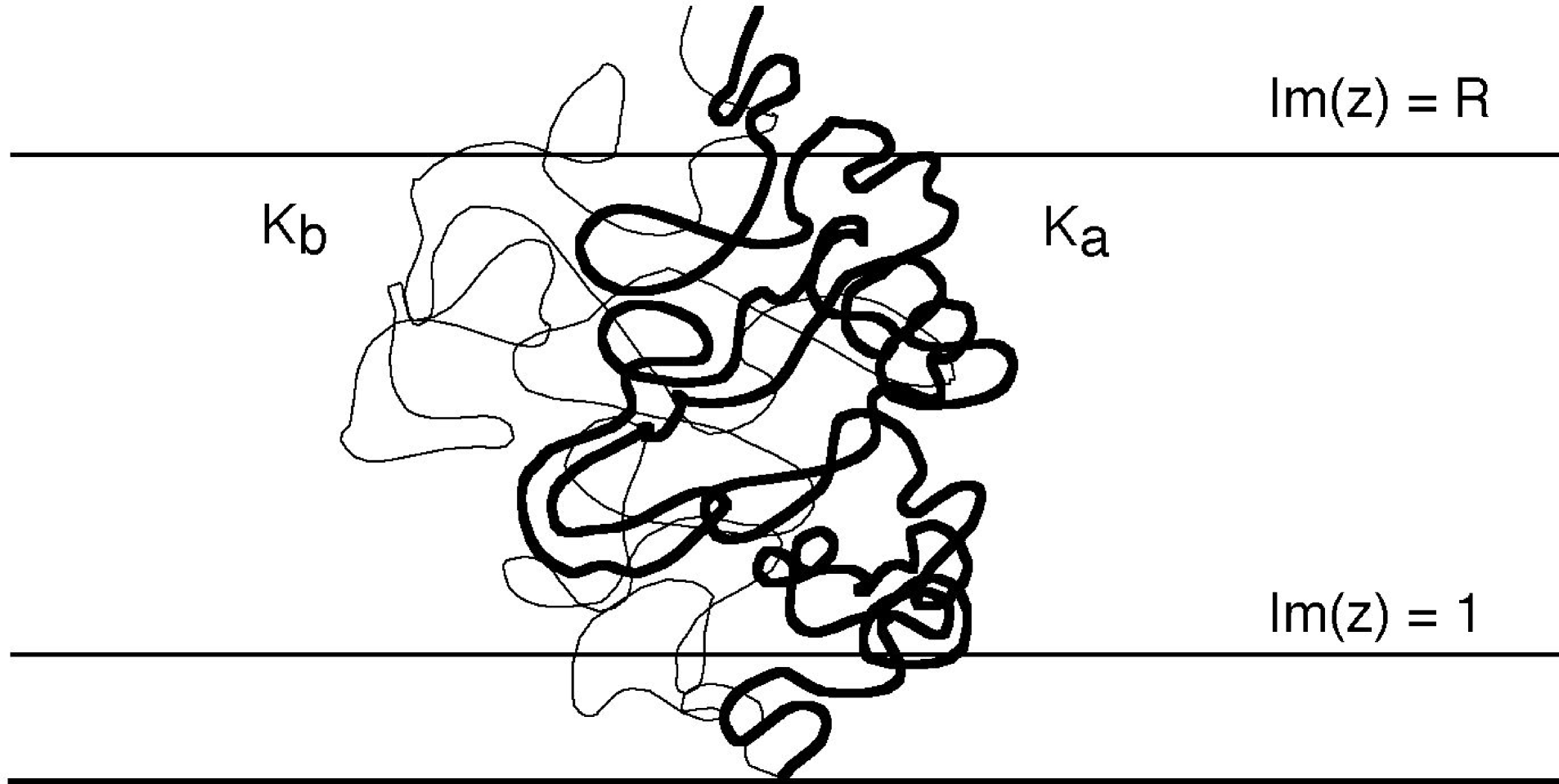
This exponent has been constructed to describe the decay in the probability that one sample of a restriction measure avoids the right boundary of another: that is, the second sample hides the first from one side of the half-plane. To be explicit, consider independent one-sided restriction measure samples and indexed by their exponents. Then the probability that the right boundary of in the strip contains no points in decays like as where is as in equation (11). This scenario is illustrated in Figure 1.
As a special case of the last, let . In this case both and are simple independent paths and the hiding condition is equivalent to mutual avoidance. We look now to iterate the above calculations, motivated by the desire to deal with several mutually avoiding paths.
3.2 Several paths in the half-plane
If we now condition on the hiding event, the right boundary of becomes an process. This can be viewed as the right boundary of a new one-sided restriction measure and we can in turn investigate the probability that this is hidden by another restriction sample to its right. In this way the process that gave us the hiding exponents can be iterated.
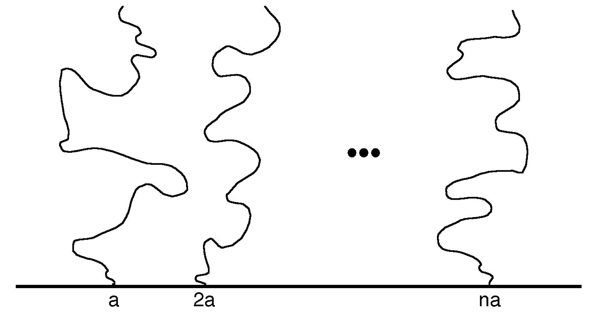
In particular, consider independent started at points , , … , on the real line and conditioned not to intersect, as depicted in Figure 2. The rightmost is an , which is the right boundary of a one-sided restriction measure of exponent . To begin we have and . Furthermore from the previous results (8) and (7)
| (12) | |||||
| (13) |
which are further simplified when we put . It now follows that
| (14) | |||||
| (15) |
The final restriction exponent differs from the expected for independent (and possibly intersecting) by
| (16) |
We conclude that the probability that these independent are mutually avoiding scales like as . This corresponds to the self-avoiding walk (SAW) exponents of Duplantier and Saleur [16] in the following fashion (assuming the SAW correspondence).
-
•
View as characterizing the step size for the SAWs and as the number of steps. Since and hence SAW have fractal dimension , the probability the SAW are mutually avoiding scales like raised to the power of as .
-
•
From [8] (using techniques) the number of SAWs in the half-plane scales like raised to the power of as .
-
•
Therefore, the number of configurations of independent and mutually avoiding self-avoiding walks scales like to the sum of these exponents, that is
This is precisely the result arrived at by Duplantier and Saleur [16].
4 Wedge exponents
We now extend exponents in the half-plane to a wedge-shaped geometry with internal wedge angle for . As a byproduct of each earlier exponent calculation, the law of the right boundary of our collection of curves was given in terms of a one-sided restriction measure, let this be of exponent for the time being. Also assume, by translating if necessary, that the right boundary begins at the origin. As in Figure 3, draw a ray starting at on the real line, of length , and making angle with the negative real line. The collection of curves avoids this ray if and only if its right boundary does, a probability which we now calculate using the restriction property.
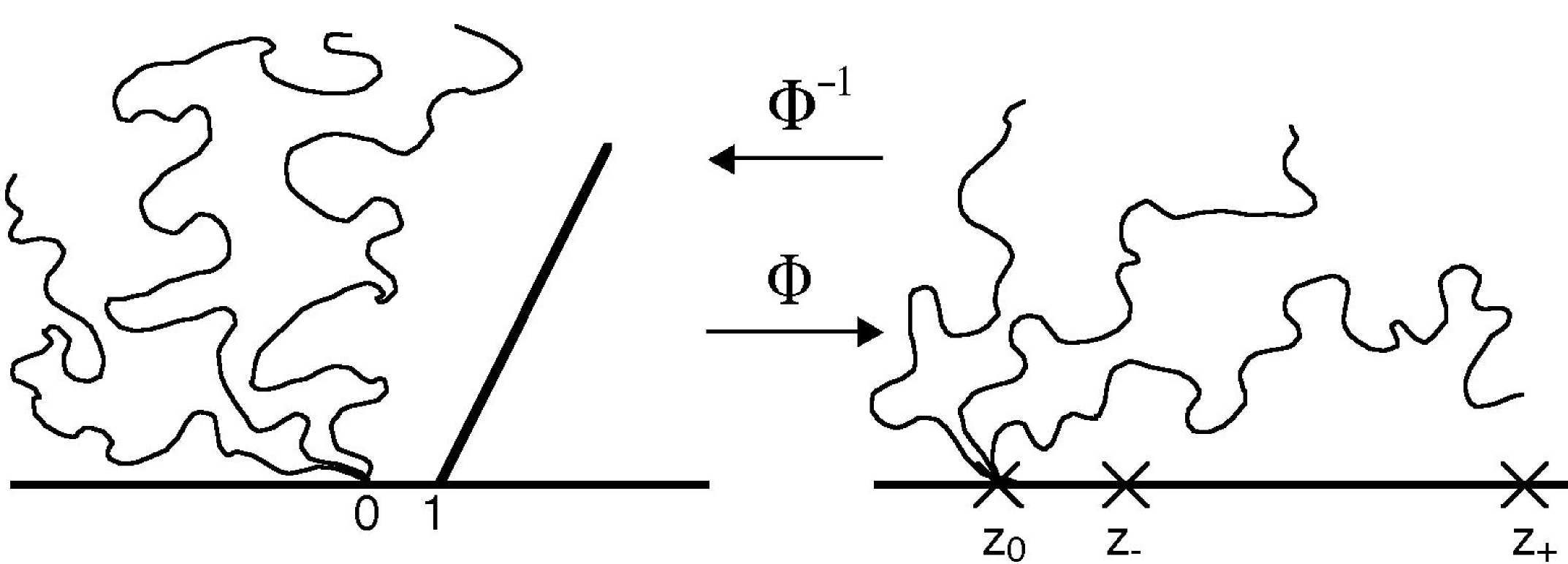
A conformal map from the half-plane to the half-plane minus the ray is
| (17) |
From (17) it is clear that as . Note that will also fix infinity, but not zero. However we can consider which will fix zero, infinity and scale like for large . Then the restriction property tells us that
| (18) | |||||
Thus all that remains is to find . This is easier said than done, since as given in (17) is difficult to invert. In light of this we use the inverse function theorem to write
| (19) |
where . First consider the behaviour of for large . From (17), extends to map both and to . This implies that . Writing as for large (and some coefficient and exponent ) and noting that
| (20) |
it follows that . As a consequence we can conclude that , as otherwise the right hand side is dominated by a positive power of as . Since we are interested only in the scaling behaviour, assume without loss of generality that . Continuing, we have . Applying the binomial theorem to the right it is clear that dominates as tends to infinity. As the left hand side states this dominant exponent must be zero,
| (21) |
Having established the behaviour of for large we now differentiate to find . Note that
| (22) |
Evaluating this at and making use of (20) gives
| (23) |
Applying the binomial theorem for large and arguing as above implies that
| (24) |
We now combine the restriction property, inverse function theorem and our expression (21) for in terms of , the ray opening angle. From this set of calculations, the probability that our collection of curves avoids the ray scales as
| (25) |
This computation is now used to extend the half-plane exponents to the wedge.
4.1 Several in a wedge
We view the probability of avoiding the ray as equivalent to the probability that of radius stays within the wedge of the same depth. To see how this probability scales with , recall that the rightmost has restriction exponent given by (15) and fractal dimension . Thus this probability decays like
| (26) |
This exponent may be added to the counting exponent in the half-plane to obtain the analogous counting exponent in the wedge, with where
| (27) |
This is precisely the set of exponents obtained by Duplantier and Saleur [16]. However, as we have used rigorous techniques, this derivation is complete modulo the assumption that is indeed the continuum limit of the self-avoiding random walk.
4.2 Hiding exponents
As an indication of the generality of these arguments, we now extend the new class of hiding exponents introduced by Werner already discussed in the half-plane. Again, it is a straightforward calculation. Return to the situation as illustrated in Figure 1. From (10) the boundary of is an where
| (28) |
Now using (8) and the above we can condition the boundary to hide another restriction measure of exponent which makes it an where
| (29) |
Turning to (7) this may be viewed as a sample of one-sided restriction measure of exponent
| (30) |
It follows that the probability that the two restriction samples stay inside the wedge will scale like
| (31) |
We therefore conclude that the hiding exponent in the wedge is simply , where is the corresponding exponent in the half-plane. This simple procedure can be extended to all exponents described with [12], extending each result to wedge geometries.
5 Conclusion
The formalism is known to provide an ideal framework in which to investigate the properties of various random curves. When coupled with the restriction property and absolute continuity relations governing , an iterative approach allows easy exploration of several mutually avoiding interfaces. Indeed, as shown, a wealth of exponents for the self-avoiding random walk, a notoriously difficult problem, can be established modulo the assumption that is the continuum limit for the self-avoiding walk. Although making this assumption may seem to detract from the otherwise rigorous nature of , the potential importance of simply as a calculational tool should not be neglected. It was with considerable ingenuity that so many exponents for the self-avoiding walk were able to be established using general arguments combined with scaling dimensions obtained using Coulomb gas and later Bethe Ansatz techniques (see for example [14, 15, 16, 20, 21]). The ease with which some of these exponents follow from the approach is not to be taken for granted.
An additional benefit of , as also illustrated in this paper, is its ability to provide new results, as well as confirming older ones. The hiding exponents first introduced by Werner [12] have been extended to wedge geometries, and more generally this paper indicates how the iterative process first outlined by Werner may be coupled with the restriction property. This provides exponents for the joint behaviour of several restriction measures in geometries contained within the half-plane. Special cases such as restriction seem crucial to generalising the powerful tools of the project to multiple or multiply connected domains where lacks a natural definition [22].
References
References
- [1] Kager W and Nienhuis B 2004 A guide to stochastic Loewner evolution and its applications J. Stat. Phys. 115 1149-1229
- [2] Lawler G 2005 Conformally Invariant Processes in the Plane Mathematical Surveys and Monographs 114 (American Mathematical Society)
- [3] Cardy J 2005 SLE for theoretical physicists Ann. of Phys. 318 81-118
- [4] Bauer M and Bernard D 2006 2D growth processes: SLE and Loewner chains Phys. Rep. 432 115-221
- [5] Cardy J L 1992 Critical percolation in finite geometries J. Phys. A: Math. Gen.25 L201-L206
- [6] Lawler G F, Schramm O and Werner W 2001 Values of Brownian intersection exponents I: Half-plane exponents Acta Mathematica 187 237-273
- [7] Lawler G F, Schramm O and Werner W 2001 Values of Brownian intersection exponents II: Plane exponents Acta Mathematica 187 275-308
- [8] Lawler G F, Schramm O and Werner W 2004 On the scaling limit of planar self-avoiding walk Proceedings of Symposia in Pure Mathematics 72.2 339-364
- [9] Kennedy T 2002 Monte Carlo tests of SLE predictions for the 2D self-avoiding walk Phys. Rev. Lett. 88 130601
- [10] Kennedy T 2004 Conformal invariance and stochastic Loewner evolution predictions for the 2D self-avoiding walk – Monte Carlo tests J. Stat. Phys. 114 51-78
- [11] Lawler G F, Schramm O and Werner W 2003 Conformal restriction: the chordal case J. American Math. Society 16 917-955
- [12] Werner W 2004 Girsanov’s transformation for processes, intersection exponents and hiding exponents Annales de la Faculté des Sciences de Toulouse 13 121-147
- [13] Duplantier B 2004 Conformal fractal geometry and boundary quantum gravity Proceedings of Symposia in Pure Mathematics 72.2 365-482
- [14] Cardy J L 1984 Conformal invariance and surface critical behavior Nucl. Phys. B 240 514-532
- [15] Cardy J L and Redner S 1984 Conformal invariance and self-avoiding walks in restricted geometries J. Phys. A: Math. Gen.17 L933-L938
- [16] Duplantier B and Saleur H 1986 Exact surface and wedge exponents for polymers in two dimensions Phys. Rev. Lett. 57 3179-3182
- [17] Rohde S and Schramm O 2005 Basic properties of SLE Ann. Math. 161 879-920
- [18] Beffara V 2003 The dimension of the SLE curves arXiv:math/0211322
- [19] Dubédat J 2005 martingales and duality, Ann. Prob. 33 223-243
- [20] Batchelor M T and Suzuki J 1993 Exact solution and surface critical behaviour of an O(n) model on the honeycomb lattice J. Phys. A: Math. Gen.26 L729-L735
- [21] Batchelor M T, Bennett-Wood D and Owczarek A L 1998 Two-dimensional polymer networks at a mixed boundary: Surface and wedge exponents Eur. Phys. J. B 5 139-142
- [22] Cardy J 2007 ADE and SLE J. Phys. A: Math. Theor. 40 1427-1438