${{~{}}^{{}^{{}^{Published~{}in~{}the~{}Journal~{}of~{}Geophysical~{}Research\,-\,Planets\,,~{}Vol.\,112\,,~{}p.\,E12003~{}\,(2007)}}}}$
${{~{}~{}~{}~{}~{}~{}~{}~{}~{}~{}~{}~{}~{}~{}~{}~{}~{}~{}~{}~{}~{}~{}~{}~{}~{}~{}~{}~{}~{}~{}~{}~{}~{}~{}~{}~{}~{}~{}~{}~{}~{}~{}~{}~{}~{}~{}~{}~{}~{}~{}~{}~{}~{}~{}~{}~{}}^{{}^{{}^{{doi}:~{}10.1029/2007JE002908}}}}$
The Physics of Bodily Tides in Terrestrial Planets,
and the Appropriate Scales of Dynamical Evolution

Abstract

Any model of tides is based on a specific hypothesis of how lagging depends on the tidal-flexure frequency $\chi$. For example, Gerstenkorn (1955), MacDonald (1964), and Kaula (1964) assumed constancy of the geometric lag angle $\,\delta\,$, while Singer (1968) and Mignard (1979, 1980) asserted constancy of the time lag $\,\Delta t\,$. Thus, each of these two models was based on a certain law of scaling of the geometric lag: the Gerstenkorn-MacDonald-Kaula theory implied that $\,\delta\,\sim\,\chi^{0}\,$, while the Singer-Mignard theory postulated $\,\delta\,\sim\,\chi^{1}$.

The actual dependence of the geometric lag on the frequency is more complicated and is determined by the rheology of the planet. Besides, each particular functional form of this dependence will unambiguously fix the appropriate form of the frequency dependence of the tidal quality factor, $\,Q(\chi)$. Since at present we know the shape of the function $\,Q(\chi)\,$, we can reverse our line of reasoning and single out the appropriate actual frequency-dependence of the lag, $\,\delta(\chi)\,$: as within the frequency range of our concern, $\,Q\,\sim\,\chi^{\alpha}\,,\;\alpha\,=\,0.2\,-\,0.4\,$, then $\,\delta\,\sim\,\chi^{-\,\alpha}\,$. This dependence turns out to be different from those employed hitherto, and it entails considerable alterations in the time scales of the tide-generated dynamical evolution. Phobos’ fall on Mars is an example we consider.

1 Introduction

If a satellite is located at a planetocentric position $\vec{r}$, it generates a tidal bulge that either advances or retards the satellite motion, depending on the interrelation between the planetary spin rate $\omega_{p}$ and the tangential part of satellite’s velocity $\vec{v}$ divided by $r\equiv|\mbox{{\boldmath$\vec{r}$}}|$. It is convenient to imagine (as on Fig. 1) that the bulge emerges beneath a fictitious satellite located at

$$\mbox{{\boldmath$\vec{r}$}}_{f}\,=\,\mbox{{\boldmath$\vec{r}$}}\,+\,\mbox{\boldmath$\vec{\boldmath{\,f}}$}\;\;\;,$$ (1)

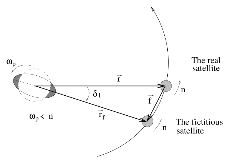
Figure 1: A planet and a tide-raising moon. This picture illustrates the case of a satellite located below the synchronous orbit, so that its mean motion $\,n\,$ exceeds the planet’s spin rate $\,\omega_{p}\,$, and the tidal bulge is lagging. The angular lag defined as $\,\delta\,\equiv\,{\textstyle{|\mbox{{\boldmath$\vec{f}$}}|}}/{\textstyle{r}}\,=\,\frac{\textstyle\Delta t}{\textstyle{r}}\,|\,\mbox{{\boldmath$\vec{\omega}$}}_{p}\times\mbox{{\boldmath$\vec{r}$}}\;-\;\mbox{{\boldmath$\vec{v}$}}\,|\,$ will, generally, differ from the absolute value of the angle $\,\delta_{1}\,$ subtended at the planet’s centre between the directions to the satellite and the bulge. Since in our study we consider an example with a small eccentricity and inclination, we make no distinction between $\,\delta\,$ and $\,|\delta_{1}|\,$.

where the position lag  $\vec{\boldmath{\,f}}$  is given by

$${\vec{\mbox{\it{f}}}}\;=\;\Delta t\;\left(\;\mbox{{\boldmath$\vec{\omega}$}}_{p}\times\mbox{{\boldmath$\vec{r}$}}\;-\;\mbox{{\boldmath$\vec{v}$}}\;\right)\;\;\;.$$ (2)

$\Delta t\,$ is the time lag between the real and fictitious tide-generating satellites, and the inclination and eccentricity of the satellite are assumed sufficiently small.

The fictitious satellite is merely a way of illustrating the time lag between the tide-raising potential and the distortion of the body. This concept implies no new physics, and is but a convenient metaphor employed to convey that at each instance of time the dynamical tide is modeled with a static tide where all the time-dependent variables are shifted back by $\,\Delta t\,$, i.e., (a) the moon is rotated back by $\,\mbox{{\boldmath$\vec{v}$}}\,\Delta t\,$, and (b) the attitude of the planet is rotated back by $\,\mbox{{\boldmath$\vec{\omega}$}}_{p}\,\Delta t\,$. From the viewpoint of a planet-based observer, this means that a dynamical response to a satellite located at  $\vec{r}$  is modeled with a static response to a satellite located at $\,\mbox{{\boldmath$\vec{r}$}}_{f}\,\equiv\,\mbox{{\boldmath$\vec{r}$}}\,-\,\Delta t\,(\mbox{{\boldmath$\vec{v}$}}\,-\,\mbox{{\boldmath$\vec{\omega}$}}_{p}\times\mbox{{\boldmath$\vec{r}$}})\,$.

In this paper, we intend to dwell on geophysical issues – the frequency-dependence of the attenuation rate and its consequences. Hence, to avoid unnecessary mathematical complications, in the subsequent illustrative example we shall restrict ourselves to the simple case of a tide-raising satellite on a near-equatorial near-circular orbit. In this approximation , the velocity of the satellite relative to the surface is

$$|\,\mbox{{\boldmath$\vec{\omega}$}}_{p}\times\mbox{{\boldmath$\vec{r}$}}~{}-~{}\mbox{{\boldmath$\vec{v}$}}\,|~{}=\;r\;|\,\omega_{p}\,-\,n\,|\;\;\;,$$ (3)

the principal tidal frequency is

$$\chi\;=\;2\;|\,\omega_{p}\,-\,n\,|\;\;\;\;,$$ (4)

and the angular lag is

$$\delta\;=\;\frac{\Delta t}{r}\;|\,\mbox{{\boldmath$\vec{\omega}$}}_{p}\times\mbox{{\boldmath$\vec{r}$}}\;-\;\mbox{{\boldmath$\vec{v}$}}\,|\;=\;\frac{\Delta t}{2}\;\chi\;\;\;,$$ (5)

$n\,$ being the satellite’s mean motion, and $\,\mbox{{\boldmath$\vec{\omega}$}}_{p}\,$ being the planet’s spin rate. The factor of two emerges in (4) since the moon causes two elevations on the opposite sides of the planet. It will also be assumed that $\;\chi\Delta t\,\ll\,1\;$, for which reason we shall neglect the second-order difference between the expression (5) and the angle subtended at the planet’s centre between the moon and the tidal bulge (rigorously speaking, the sine of the subtended angle is equal to $\;\mbox{{\boldmath$\vec{f}$}}\,\times\,\mbox{{\boldmath$\vec{r}$}}/r^{2}\;$).

The starting point of all tidal models is that each elementary volume of the planet is subject to a tide-raising potential, which in general is not periodic but can be expanded into a sum of periodic terms. Within the linear approximation introduced by Love, the tidal perturbations of the potential yield linear response of the shape and linear variations of the stress. In extension of the linearity approximation, it is always implied that the overall dissipation inside the planet may be represented as a sum of attenuation rates corresponding to each periodic disturbance:

$$\langle\,\dot{E}\;\rangle\;=\;\sum_{i}\;\langle\,\dot{E}(\chi_{\textstyle{{}_{i}}})\;\rangle$$ (6)

where, at each frequency $\,\chi_{i}\,$,

$$\langle\,\dot{E}(\chi_{\textstyle{{}_{i}}})~{}\rangle~{}=~{}-~{}2~{}\chi_{\textstyle{{}_{i}}}~{}\frac{\,\langle\,E(\chi_{\textstyle{{}_{i}}})~{}\rangle\,}{Q(\chi_{\textstyle{{}_{i}}})}~{}=\,\;-\;\chi_{\textstyle{{}_{i}}}\;\frac{\,E_{{}_{peak}}(\chi_{\textstyle{{}_{i}}})\,}{Q(\chi_{\textstyle{{}_{i}}})}\;\;\;,$$ (7)

$\langle\,.\,.\,.\,\rangle~{}$ standing for averaging over flexure cycle, $\,E(\chi_{\textstyle{{}_{i}}})\,$ denoting the energy of deformation at the frequency $\,\chi_{\textstyle{{}_{i}}}\,$, and $Q(\chi_{\textstyle{{}_{i}}})\,$ being the quality factor of the material at this frequency. Introduced empirically as a means to figleaf our lack of knowledge of the attenuation process in its full complexity, the notion of $\,Q\,$ has proven to be practical due to its smooth and universal dependence upon the frequency and temperature. An alternative to employment of the empirical $\,Q\,$ factors would be comprehensive modeling of dissipation using a solution of the equations of motion, given a rheological description of the mantle (Mitrovica & Peltier 1992; Hanyk, Matyska & Yuen 1998, 2000; Moore & Schubert 2000). Though providing a valuable yield for a geophysicist, this comprehensive approach may be avoided in astronomy, where only the final outcome, the frequency dependence of $\,Q\,$, is important. Fortunately, this dependence is already available from observations.

In this paper we shall restrict ourselves to the simple case of an equatorial or near-equatorial satellite describing a circular or near-circular orbit. Under these circumstances only the principal tidal frequency (4) will matter.

2 The quality factor $Q$ and the geometric lag angle $\delta$.

During tidal flexure, the energy attenuation through friction is, as ever, accompanied by a phase shift between the action and the response. The tidal quality factor is interconnected with the phase lag $\,\epsilon$ and the angular lag $\delta\,$ via

$$Q^{-1}\;=\;\tan\epsilon\;=\;\tan 2\delta$$ (8)

or, for small lag angles,

$$Q^{-1}\;\approx\;\epsilon\;=\;2\;\delta\;\;\;.~{}~{}$$ (9)

The doubling of the lag is a nontrivial issue. Many authors erroneously state that $\,Q^{-1}\,$ is equal simply to the tangent of the lag, with the factor of two omitted. For example, Rainey & Aharonson (2006) assume that $\,Q^{-1}\,$ is equal to the tangent of the geometric lag. As a result, they arrive at a value of $\,Q\,$ that is about twice larger than those obtained by the other teams. In Bills et al. (2005), one letter, $\,\gamma\,$, is used to denote two different angles. Prior to equation (24) in that paper, $\,\gamma\,$ signifies the geometric lag (in our notations, $\,\delta_{1}\,$). Further, in their equations (24) and (25), Bills et al. employ the notation $\,\gamma\,$ to denote the phase lag (in our notations, $\,\epsilon\,$, which happens to be equal to $\,2\,\delta_{1}\,$). With this crucial caveat, Bills’ equation $\,Q\,=\,1/\tan\gamma\,$ is correct. This inaccuracy in notations has not prevented Bills et al. (2005) from arriving to a reasonable value of the Martian quality factor, $\,85.58\pm 0.37\,$. (A more recent study by Lainey et al. (2007) has given a comparable value of $\,79.91\pm 0.69\,$.)

In the Appendix, we offer a simple illustrative calculation, which explains whence this factor of two stems.

Formulae (8 - 9) look reasonable: the higher the quality factor, the lower the damping rate and, accordingly, the smaller the lag. What looks very far from being OK are the frequency dependencies ensuing from the assertions of $\,\delta\,$ being either constant or linear in frequency: the approach taken by Gerstenkorn (1955), MacDonald (1964), and Kaula (1964) implies that $\,Q\,\sim\,\chi^{0}\,$, while the theory of Singer (1968) and Mignard (1979, 1980) yields $\,Q\,\sim\,\chi^{-1}\,$, neither option being in agreement with the geophysical data.

3 Dissipation in the mantle.

3.1 Generalities

Back in the 60s and 70s of the past century, when the science of low-frequency seismological measurements was yet under development, it was widely thought that at long time scales the quality factor of the mantle is proportional to the inverse of the frequency. This fallacy proliferated into planetary astronomy where it was received most warmly, because the law $\,Q\,\sim\,1/\chi\,$ turned out to be the only model for which the linear decomposition of the tide gives a set of bulges displaced from the direction to the satellite by the same angle. Any other frequency dependence $\,Q(\chi)\,$ entails superposition of bulges corresponding to the separate frequencies, each bulge being displaced by its own angle. This is the reason why the scaling law $\,Q\,\sim\,1/\chi\,$, long disproved and abandoned in geophysics (at least, for the frequency band of our concern), still remains a pet model in celestial mechanics of the Solar system.

Over the past twenty years, considerable progress has been achieved in the low-frequency seismological measurements, both in the lab and in the field. Due to an impressive collective effort undertaken by several teams, it is now a firmly established fact that for frequencies down to about $\sim 1$ yr^-1 the quality factor of the mantle is proportional to the frequency to the power of a positive fraction $\,\alpha\,$. This dependence holds for all rocks within a remarkably broad band of frequencies: from several MHz down to about $\;1\;$yr${}^{-1}\,$.

At timescales longer than $\,1$ yr, all the way to the Maxwell time (about $\,100$ yr), attenuation in the mantle is defined by viscosity, so that the quality factor is, for all minerals, well approximated with $\,{\eta}\chi/M\,$, where $\eta$ and $M$ are the shear viscosity and the shear elastic modulus of the mineral. Although the values of both the viscosity coefficients and elastic moduli greatly vary for different minerals and are sensitive to the temperature, the overall quality factor of the mantle at such long timescales still is linear in frequency.

At present there is no consensus in the seismological community in regard to the time scales exceeding the Maxwell time. One viewpoint (incompatible with the Maxwell model) is that the linear law $\,Q\,\sim\,\chi\,$ extends all the way down to the zero-frequency limit (Karato 2007). An alternative point of view (prompted by the Maxwell model) is that at scales longer than the Maxwell time we return to the inverse-frequency law $\,Q\,\sim\,1/\chi\,$.
 
All in all, we have:

$$\mbox{For}\;\;\;\;\;\;10^{7}\;\;\mbox{Hz}\;\;>\,\;\chi\;\;>\;\;1\;yr^{-1}\;:\;\;\;Q\,\sim\,\chi^{\alpha}\;,\,\;\mbox{with}\;\,\alpha\,=\,0.2\,-\,0.4\;\;\;(\,0.2\;\mbox{for partial melts})\;.\;\;\;\,$$ (10)

$$\mbox{For}\;\;\;\;\;\;\;\;\;1\;yr^{-1}\,>\,\chi\,>\,10^{-2}\,\;yr^{-1}\;\;:\;\;\;\;Q\,\sim\,\chi\;\;\;.\;\;\;\;~{}~{}~{}~{}~{}~{}~{}~{}~{}~{}~{}~{}~{}~{}~{}~{}~{}~{}~{}~{}~{}~{}~{}~{}~{}~{}~{}~{}~{}~{}~{}~{}~{}~{}~{}~{}~{}~{}~{}~{}~{}~{}~{}~{}~{}~{}~{}~{}~{}~{}~{}~{}~{}~{}~{}~{}~{}~{}$$ (11)

$$\mbox{For}\;\;\;\;\;10^{-2}\;yr^{-1}\,>\,\chi\;:\;\;\;\mbox{arguably, ~{}it ~{}is ~{}still~{}~{}}Q\,\sim\,\chi\;.\;\;\;\;\;(\,\mbox{Or~{}maybe~{}~{}~{}}Q\;\sim\;1/\chi~{}\,?\,)~{}~{}~{}~{}~{}~{}~{}~{}~{}~{}~{}~{}~{}\,$$ (12)

Fortunately, in practical calculations of tides in planets one never has to transcend the Maxwell time scales, so the controversy remaining in (12) bears no relevance to our subject. We leave for a future study the case of synchronous satellites, the unique case of the Pluto-Charon resonance, or the binary asteroids locked in the same resonance. Thus we shall avoid also the frequency band addressed in (11), but shall be interested solely in the frequency range described in (10). It is important to emphasise that the positive-power scaling law (10) is well proven not only for samples in the lab but also for vast seismological basins and, therefore, is universal. Hence, this law may be extended to the tidal friction – validity of this extension will be discussed below in subsection 3.4.1

Below we provide an extremely condensed review of the published data whence the scaling law (10) was derived by the geophysicists. The list of sources will be incomplete, but a full picture can be obtained through the further references contained in the works to be quoted below. For a detailed treatment, see Chapter 11 of the book by Karato (2007) that contains a systematic introduction into the theory of and experiments on attenuation in the mantle.

3.2 Circumstantial evidence: attenuation in minerals.
Laboratory measurements and some theory

Even before the subtleties of solid-state mechanics with or without melt are brought up, the positive sign of the power $\,\alpha\,$ in the dependence $\,Q\,\sim\,\chi^{\alpha}\,$ may be anticipated on qualitative physical grounds. For a damped oscillator obeying $\;\ddot{z}\,+\,2\,\beta\,\dot{z}\,+\,\chi^{2}\,z\,=\,0\;\,$, the quality factor is equal to $\,\chi/(2\beta)\,$, i.e., $\,Q\,\sim\,\chi\,$.

Solid-state phenomena causing attenuation in the mantle may be divided into three groups: the point-defect mechanisms, the dislocation mechanisms, and the grain-boundary ones.

Among the point-defect mechanisms, most important is the transient diffusional creep, i.e., plastic flow of vacancies, and therefore of atoms, from one grain boundary to another. The flow is called into being by the fact that vacancies (as well as the other point defects) have different energies at grain boundaries of different orientation relative to the applied shear stress. This anelasticity mechanism is wont to obey the power law $\,Q\,\sim\,\chi^{\alpha}\,$ with $\,\alpha\,\approx\,0.5\,$.

Anelasticity caused by dislocation mechanisms is governed by the viscosity law $\,Q\,\sim\,\chi\,$ valid for sufficiently low frequencies (or sufficiently high temperatures), i.e., when the viscous motion of dislocations is not restrained by the elastic restoring stress. (At higher frequencies or/and lower temperatures, the restoring force “pins” the defects. This leads to the law $\,Q\,\sim\,(\textstyle{1\,+\,\tau^{2}\chi^{2}})\tau^{-1}\chi^{-1}\,$, parameter $\,\tau\,$ being the relaxation time whose values considerably vary among different mechanisms belonging to this group. As the mantle is warm and viscous, we may ignore this caveat.)

The grain-boundary mechanisms, too, are governed by the law $\,Q\sim\chi^{\alpha}$, though with a lower exponent: $\,\alpha\approx 0.2-0.3$. This behaviour gradually changes to the viscous mode ($\alpha=1$) at higher temperatures and/or at lower frequencies, i.e., when the elastic restoring stress reduces.

We see that in all cases the quality factor of minerals should grow with frequency. Accordingly, laboratory measurements confirm that, within the geophysically interesting band of $\,\chi\,$, the quality factor behaves as $\,Q\,\sim\,\chi^{\alpha}\,$ with $\,\alpha\,=\,0.2\,-\,0.4\;$. Such measurements have been described in Karato & Spetzler (1990) and Karato (1998). Similar results were reported in the works by the team of I. Jackson – see, for example, the paper (Tan et al. 1997) where numerous earlier publications by that group are also mentioned.

In aggregates with partial melt the frequency dependence of $\,Q\,$ keeps the same form, with $\,\alpha\,$ leaning to $\,0.2\,$ – see, for example, Fontaine et al. (2005) and references therein.

3.3 Direct evidence: attenuation in the mantle.
Measurements on seismological basins

As we are interested in the attenuation of tides, we should be prepared to face the possible existence of mechanisms that may show themselves over very large geological structures but not in small samples explored in the lab. No matter whether such mechanisms exist or not, we would find it safer to require that the positive-power scaling law $\,Q\,\sim\,\chi^{\alpha}\,$, even though well proven in the lab, must be propped up by direct seismological evidence gathered over vast zones of the mantle. Fortunately, such data are available, and for the frequency range of our interest these data conform well with the lab results. The low-frequency measurements, performed by different teams over various basins of the Earth’s upper mantle, agree on the pivotal fact: the seismological quality factor scales as the frequency to the power of a positive fraction $\,\alpha\;$ – see, for example, Mitchell (1995), Stachnik et al. (2004), Shito et al. (2004), and further references given in these sources.

3.4 Consequences for the tides

3.4.1 Tidal dissipation vs seismic dissipation

For terrestrial planets, the frequency-dependence of the $\,Q\,$ factor of bodily tides is similar to the frequency-dependence (10 - 11) of the seismological $\,Q\,$ factor. This premise is based on the fact that the tidal attenuation in the mantle is taking place, much like the seismic attenuation, mainly due to the mantle’s rigidity. This is a nontrivial fact because, in distinction from earthquakes, the damping of tides is taking place both due to nonrigidity and self-gravity of the planet. Modeling the planet with a homogeneous sphere of density $\,\rho\,$, rigidity $\,\mu\,$, surface gravity  g , and radius $\,R\,$, Goldreich (1963) managed to separate the nonrigidity-caused and self-gravity-caused inputs into the overall tidal attenuation. His expression for the tidal quality factor has the form

$$Q\;=\;Q_{o}\left(\;1\;+\;\frac{2}{19}\;\frac{\mbox{g}\;\rho\;R}{\mu}\;\right)\;\;\;,$$ (13)

$Q_{o}\,$ being the value that the quality factor would assume were self-gravity absent. To get an idea of how significant the self-gravity-produced input could be, let us plug there the mass and radius of Mars and the rigidity of the Martian mantle. For the Earth’s mantle, $\,\mu\,=\,65\,\div\,80\,$GPa. Judging by the absence of volcanic activity over the past hundred(s) of millions of years of Mars’ history, the temperature of the Martian upper mantle is (to say the least) not higher than that of the terrestrial one. Therefore we may safely approximate the Martian $\,\mu\,$ with the upper limit for the rigidity of the terrestrial mantle: $\,\mu\,=\,10^{11}\,$Pa. All in all, the relative contribution from self-gravity will look as

$$\frac{2}{19}\;\frac{\mbox{g}\;\rho\;R}{\mu}\;=\;\frac{6}{76\,\pi}\;\frac{\gamma\;M^{2}}{\mu\;R^{4}}\;\approx\;\frac{1}{40}\;\frac{(\;6.7\,\times\,10^{\textstyle{{}^{-11}}}\,\mbox{m}^{\textstyle{{}^{3}}}\,\mbox{kg}^{\textstyle{{}^{-1}}}\,\mbox{s}^{\textstyle{{}^{-2}}}\;)\;\;(\;6.4\,\times\,10^{\textstyle{{}^{23}}}\,\mbox{kg}\;)^{\textstyle{{}^{2}}}}{(\;10^{\textstyle{{}^{11}}}\;\mbox{Pa}\;)\;\;(\;3.4\,\times\,10^{\textstyle{{}^{6}}}\,m\;)^{\textstyle{{}^{4}}}}\;\approx\;5.2\,\times\,10^{\textstyle{{}^{-2}}}\;\;,\;\;\;\;$$ (14)

$\gamma$ denoting the gravity constant. This, very conservative estimate shows that self-gravitation contributes, at most, several percent into the overall count of energy losses due to tides. This is the reason why we extend to the tidal $\,Q\,$ the frequency-dependence law measured for the seismic quality factor.

3.4.2 Dissipation in the planet vs dissipation in the satellite

A special situation is tidal relaxation toward the state where one body shows the same side to another. Numerous satellites show, up to librations, the same face to their primaries. Among the planets, Pluto does this to Charon. Such a complete locking is typical also for binary asteroids. A gradual approach toward the synchronous orbit involves ever-decreasing frequencies, eventually exceeding the limits of equation (11) and thus the bounds of the present discussion. Mathematically, this situation still may be tackled by means of (10) until the tidal frequency $\,\chi\,$ decreases to $\;1\,$yr^-1, and then by means of (11) while $\,\chi\,$ remains above the inverse Maxwell time of the planet’s material. Whether the latter law can be extended to longer time scales remains an open issue of a generic nature that is not related to a specific model of tides or to a particular frequency dependence of $\,Q\;$. The generic problem is whether we at all may use the concept of the quality factor beyond the Maxwell time, or should instead employ, beginning from some low $\,\chi\,$, a comprehensive hydrodynamical model. In the current work, we address solely the satellite-generated tides on the planet. The input from the planet-caused tides on the satellite will be considered elsewhere. The case of Pluto will not be studied here either. Nor shall we address binary asteroids. (Since at present most asteroids are presumed loosely connected, and since we do not expect the dependencies (10 - 11) to hold for such aggregates, our theory should not, without some alterations, be applied to such binaries.)

Thus, since we are talking only about dissipation inside the planet, and are not addressing the exceptional Pluto-Charon case, we may safely assume the tidal frequency to always exceed $\;1\,$yr^-1. Thence (10) will render, for a typical satellite:

$${\left.~{}~{}~{}~{}~{}~{}~{}~{}~{}\right.}Q\,\sim\,\chi^{\alpha}~{}~{}~{},~{}~{}~{}~{}\mbox{with}~{}~{}\alpha~{}=~{}0.2~{}-~{}0.4~{}~{}~{}.$$ (15)

Accordingly, (9) will entail:

$${\left.~{}~{}~{}~{}~{}~{}~{}~{}~{}\right.}\delta~{}\sim~{}\chi^{-\alpha}~{}~{}~{},~{}~{}~{}~{}\mbox{with}~{}~{}\alpha~{}=~{}0.2~{}-~{}0.4~{}~{}~{}.$$ (16)

Another special situation is a satellite crossing a synchronous orbit. At the moment of crossing, the principal tidal frequency $\,\chi\,=\,2\,|\omega_{p}\,-\,n|\,$ vanishes. As (9) and (10) yield $\,Q\,\approx\,(2\delta)^{-1}\,$ and $\,Q\,\sim\,\chi^{\alpha}\,$, then we get $\,\delta\,\sim\,\chi^{-\alpha}\,$ with a positive $\,\alpha\,$. Uncritical employment of these formulae will then make one think that at this instant the lag $\,\delta\,$ grows infinitely, a clearly nonsensical result. The quandary is resolved through the observation that the bulge is lagging not only in its position but also in its height, for which reason the dissipation rate remains finite (Efroimsky 2007). Since in this paper we shall not consider crossing of or approach to synchronous orbits, and since the example we aim at is Phobos, we shall not go deeper into this matter here.

3.5 A thermodynamical aside: the frequency and the temperature

In the beginning of the preceding subsection we already mentioned that though the tidal $Q$ differs from the seismic one, both depend upon the frequency in the same way, because this dependence is determined by the same physical mechanisms. This pertains also to the temperature dependence, which for some fundamental reason combines into one function with the frequency dependence.

As explained, from the basic physical principles, by Karato (2007, 1998), the frequency and temperature dependencies of $\,Q\,$ are inseparably connected. The quality factor can, despite its frequency dependence, be dimensionless only if it is a function not just of the frequency per se but of a dimensionless product of the frequency by the typical time of defect displacement. This time exponentially depends on the activation energy $A^{*}$, whence the resulting function is

$$Q\;\sim\;\left[\,\chi\;\exp(A^{*}/RT)\,\right]^{\alpha}\;\;\;.$$ (17)

For most minerals of the upper mantle, $A^{*}$ lies within the limits of $360-540$ kJ mol^-1. For example, for dry olivine it is about $520$ kJ mol^-1.

Thus, through formulae (17) and (9), the cooling rate of the planet plays a role in the orbital evolution of satellites: the lower the temperature, the higher the quality factor and, thereby, the smaller the lag $\,\delta\,$. For the sake of a crude estimate, assume that most of the tidal attenuation is taking place in some layer, for which an average temperature $T$ and an average activation energy $A^{*}$ may be introduced. Then from (17) we have: $\,\Delta Q/{Q}\,\approx\,-\,\alpha\,A^{*}\,\Delta T/RT\,$. For a reasonable choice of values $\,\alpha=0.3\,$ and $\,A^{*}=\,5.4\,\times\,10^{5}\,J/mol\,$, a drop of the temperature from $\,T_{o}=2000\,K\,$ down by $\,\Delta T=200\,K\,$ will result in $\,\Delta Q/Q\,\approx\,1\,$. So a $\,10\,\%\,$ decrease of the temperature can result in an about $\,100\,\%\,$ growth of the quality factor.

Below we shall concentrate on the frequency dependence solely.

4 Formulae

The tidal potential perturbation acting on the tide-raising satellite is

$$U(\delta_{1})\;=~{}\frac{A_{2}}{r_{\textstyle{{}_{f}}}^{5}\;r^{5}}\;\left(\,3\;\left(\mbox{{\boldmath$\vec{r}$}}_{f}\cdot\mbox{{\boldmath$\vec{r}$}}\right)^{2}\;-\;\mbox{{\boldmath$\vec{r}$}}_{f}^{\;2}\;\mbox{{\boldmath$\vec{r}$}}^{\;2}\,\right)\;+\;\frac{A_{3}}{r_{\textstyle{{}_{f}}}^{6}\;r^{6}}\;\left(\,5\;\left(\mbox{{\boldmath$\vec{r}$}}_{f}\cdot\mbox{{\boldmath$\vec{r}$}}\right)^{2}\;-\;3\;\mbox{{\boldmath$\vec{r}$}}_{f}^{\;2}\;\mbox{{\boldmath$\vec{r}$}}^{\;2}\,\right)\;+\;\;.\;\,.\;\,.~{}~{}$$ (18)

where $\,r\,\equiv\,|\mbox{{\boldmath$\vec{r}$}}|\,$ and $\,r_{f}\,\equiv\,|\mbox{{\boldmath$\vec{r}$}}_{f}|\,$, while the constants are given by

$$A_{2}\;\equiv\;\frac{k_{2}\,G\,m\,R^{5}}{2}\;\;\;\;,\;\;\;\;\;\;A_{3}\;\equiv\;\frac{k_{3}\,G\,m\,R^{7}}{2}\;\;\;\;,\;\;\;\;\;\;\;.\,\;.\,\;.\;\;\;\;,$$ (19)

$k_{n}\,$ being the Love numbers. (For derivation of (18) see, for example, MacDonald (1964) and literature cited therein.)

Three caveats will be appropriate at this point. First, to (18) we should add the potential due to the tidal distortion of the moon by the planet. That input contributes mainly to the radial component of the tidal force exerted on the moon, and entails a decrease in eccentricity and semi-major axis (MacDonald 1964). Here we omit this term, since our goal is to clarify the frequency dependence of the lag. Second, we acknowledge that in many realistic situations the $\,k_{3}\,$ and sometimes even the $\,k_{4}\,$ term is relevant (Bills et al. 2005). With intention to keep these inputs in our subsequent work, here we shall restrict our consideration to the leading term only. Hence the ensuing formula for the tidal force will read:

$$\mbox{{\boldmath$\vec{\cal{F}}$}}\;=\;-\;\frac{3\;k_{2}\;G\;m^{2}\;R^{5}}{r^{7}}\;\left[\;\frac{\mbox{{\boldmath$\vec{r}$}}}{r}\;-\;\frac{\vec{\mbox{\it{f}}}}{r}\;-\;2\;\frac{\mbox{{\boldmath$\vec{r}$}}}{r}\;\frac{\,\mbox{{\boldmath$\vec{r}$}}\cdot{\vec{\mbox{\it{f}}}}\,}{r^{2}}\;+\;O(\,{\mbox{{\boldmath$\vec{f}$}}}^{\;\;{2}}/r^{2})\right]\;+\;O(k_{3}Gm^{2}R^{7}/r^{9})\;\;\;$$

$$\approx\;-\;\frac{3\;k_{2}\;G\;m^{2}\;R^{5}}{r^{10}}\;\left[\;{\mbox{{\boldmath$\vec{r}$}}}\;{r^{2}}\;-\;{\vec{\mbox{\it{f}}}}\;{r^{2}}\;-\;2\;{\mbox{{\boldmath$\vec{r}$}}}\;\left(\,\mbox{{\boldmath$\vec{r}$}}\cdot{\vec{\mbox{\it{f}}}}\,\right)\;\right]\;\;\;,\;\;\;\;\;\;\;\;\;\;\;\;\;\;\;\;~{}~{}~{}~{}~{}~{}~{}~{}~{}~{}~{}~{}~{}~{}~{}~{}~{}~{}~{}~{}~{}~{}$$ (20)

The third important caveat is that in our further exploitation of this formula we shall take into account the frequency-dependence of the lag  $\vec{\boldmath{\,f}}$ , but not of the parameter $\,k_{2}\,$. While the dependence $\,\mbox{\boldmath$\vec{\boldmath{\,f}}$}(\chi)\,$ will be derived through the interconnection of  $\vec{\boldmath{\,f}}$  with $\,\delta(\chi)\,$ and therefore with $\,Q(\chi)\,$, the value of $\,k_{2}\,$ will be asserted constant. That the latter is acceptable can be proven through the following formula obtained by Darwin (1908) under the assumption of the planet being a Maxwell body (see also Correia & Laskar 2003):

$$k_{2}(\chi)\;=\;k_{\textstyle{{}_{fluid}}}\;\,\sqrt{\;\frac{1\;+\;\chi^{2}\;\eta^{2}/\mu^{2}}{1\;+\;\left(\,\chi^{2}\;\eta^{2}/\mu^{2}\,\right)\;\left(\,1\;+\;19\;\mu/(2\,g\,\rho\,R)\,\right)^{2}}\;}\;\;\;.$$

Here $\,k_{\textstyle{{}_{fluid}}}\,$ is the so-called fluid Love number. This is the value that $\,k_{2}\,$ would have assumed had the planet consisted of a perfect fluid with the same mass distribution as the actual planet. Notations $\,\mu\,$, $\,\rho\,$,  g , and  g  stand for the rigidity, mean density, surface gravity, and the radius of the planet. For these parameters, we shall keep using the estimates from subsection 3.4. The letter $\,\eta\,$ signifies the viscosity. Up to an order or two of magnitude, its value may be approximated, for a terrestrial planet’s mantle, with $\,10^{22}\,$kg/(m$\cdot$ s). This will yield: $\,\chi^{2}\;\eta^{2}/\mu^{2}\,=\,(\,\chi\,\cdot\,10^{11}\,\mbox{s}\,)^{2}\,$, wherefrom we see that in all realistic situations pertaining to terrestrial planets the frequency-dependence in Darwin’s formula will cancel out. Thus we shall neglect the frequency-dependence of the Love number $\,k_{2}\,$ (but shall at the same time take into account the frequency-dependence of $\,Q\,$, for it will induce frequency-dependence of all three lags).

The interconnection between the position, time, and angular lags,

$$\delta\;\equiv\,\;\frac{|{\vec{\mbox{\it{f}}}}\,|}{r}\,\;=\;\Delta t\;\;\frac{1}{r}\;|\;\mbox{{\boldmath$\vec{\omega}$}}_{p}\times\mbox{{\boldmath$\vec{r}$}}\;-\;\mbox{{\boldmath$\vec{v}$}}\;|\;\,=\;\frac{\Delta t}{2}\;\chi~{}~{}~{},$$ (21)

can be equivalently rewritten as:

$${\vec{\mbox{\it{f}}}}~{}=~{}{\bf{\hat{f}}}\;r\;\delta\;=\;r\;\frac{\Delta t}{2}\;\chi\;{\bf{\hat{f}}}\;\;\;,$$ (22)

where

$${\bf{\hat{f}}}\;=\;\frac{~{}\mbox{{\boldmath$\vec{\omega}$}}_{p}\times\mbox{{\boldmath$\vec{r}$}}\,-\,\mbox{{\boldmath$\vec{v}$}}}{~{}|\,\mbox{{\boldmath$\vec{\omega}$}}_{p}\times\mbox{{\boldmath$\vec{r}$}}\,-\,\mbox{{\boldmath$\vec{v}$}}\,|}$$ (23)

is a unit vector pointing in the lag direction.

Be mindful that we assume the inclination and eccentricity to be small, wherefore the ratio

$$\frac{|{\vec{\mbox{\it{f}}}}\,|}{r}\,\;=\;\Delta t\;\;\frac{1}{r}\;|\;\mbox{{\boldmath$\vec{\omega}$}}_{p}\times\mbox{{\boldmath$\vec{r}$}}\;-\;\mbox{{\boldmath$\vec{v}$}}\;|$$

is simply the tangential angular lag, i.e., the geometric angle subtended at the primary’s centre between the moon and the bulge. In the general case of a finite inclination or/and eccentricity, all our formulae will remain in force, but the lag $\,\delta\,$ will no longer have the meaning of the subtended angle.

At this point, it would be convenient to introduce a dimensional integral parameter $\,{\cal{E}}\,$ describing the overall tidal attenuation rate in the planet. The power scaling law mentioned in section 3 may be expressed as

$$Q\,=\,{\cal E}^{\alpha}\,\chi^{\alpha}~{}~{}~{},~{}~{}~{}$$ (24)

where $\,{\cal E}^{\alpha}\,$ is simply the dimensional factor emerging in the relation $\,Q\,\sim\,\chi^{\alpha}\,$. As mentioned in subsection 3.5, cooling of the planet should become a part of long-term orbital calculations. It enters these calculations through evolution of this parameter $\,{\cal{E}}\,$. Under the assumption that most of the tidal dissipation is taking place in some layer, for which an average temperature $T$ and an average activation energy $A^{*}$ may be defined, (17) yields:

$${\cal E}\;=\;{\cal E}_{o}\;\exp\left[\,\frac{A^{*}}{R}\;\left(\,\frac{1}{T_{o}}\;-\;\frac{1}{T}\;\right)\;\right]\;\;\;,$$

$T_{o}\,$ being the temperature of the layer at some fiducial epoch. The physical meaning of the integral parameter $\,{\cal{E}}\,$ is transparent: if the planet were assembled of a homogeneous medium, with a uniform temperature distribution, and if attenuation in this medium were caused by one particular physical mechanism, then $\,{\cal{E}}\,$ would be a relaxation time scale associated with this mechanism (say, the time of defect displacement). For a realistic planet, $\,{\cal{E}}\,$ may be interpreted as a relaxation time averaged (in the sense of $\,Q\,=\,{\cal E}^{\alpha}\,\chi^{\alpha}\,$) over the planet’s layers and over the various damping mechanisms acting within these layers.

As (10) entails $\;\delta\,\approx\,1/(2\,Q)\,=\,(1/2)\,{\cal{E}}^{-\alpha}\,\chi^{-\alpha}\;$, then (21) necessitates for the position lag:

$${\vec{\mbox{\it{f}}}}~{}=~{}r\;\delta\;{\bf{\hat{f}}}\;=\;\frac{1}{2}\;r\;{\cal E}^{-\alpha}\;\chi^{-\alpha}\;{\bf{\hat{f}}}\;\;\;,$$ (25)

and for the time lag:

$${\Delta t}\;=\;{\cal E}^{-\alpha}\;\chi^{-(\alpha+1)}\;\;\;,$$ (26)

${\cal E}\,$ being the planet’s integral parameter introduced above, and $\,\chi\,$ being a known function (4) of the orbital variables. Putting everything together, we arrive at

$${\vec{\mbox{\it{f}}}}~{}=\,\frac{1}{2}\,\left({\cal{E}}{\chi}\right)^{-\alpha}\,a\;\,\frac{1\,-\,e^{2}}{1\,+\,e\;\cos\nu}\;\,\frac{~{}\mbox{{\boldmath$\vec{\omega}$}}_{p}\times\mbox{{\boldmath$\vec{r}$}}\,-\,\mbox{{\boldmath$\vec{v}$}}~{}}{~{}|\,\mbox{{\boldmath$\vec{\omega}$}}_{p}\times\mbox{{\boldmath$\vec{r}$}}\,-\,\mbox{{\boldmath$\vec{v}$}}\,|~{}}~{}=~{}\frac{1}{2}\,\left({\cal{E}}{\chi}\right)^{-\alpha}\,a\;\,\frac{~{}\mbox{{\boldmath$\vec{\omega}$}}_{p}\times\mbox{{\boldmath$\vec{r}$}}\,-\,\mbox{{\boldmath$\vec{v}$}}~{}}{~{}|\,\mbox{{\boldmath$\vec{\omega}$}}_{p}\times\mbox{{\boldmath$\vec{r}$}}\,-\,\mbox{{\boldmath$\vec{v}$}}\,|~{}}\;+\;O(e)\;\;,~{}~{}$$ (27)

where

$$\chi\,\equiv\;2\;|\omega_{p}\,-\;n|\;\;.\;\;$$ (28)

The time lag is, according to (26):

$$\Delta t={\cal{E}}\;\left(\,2\;{\cal{E}}\;|\omega_{p}\,-\;n|\,\right)^{\textstyle{{}^{-\,(\alpha+1)}}}.~{}$$ (29)

Formulae (29), (27), and (20) are sufficient to both compute the orbit evolution and trace the variations of the time lag.

5 The example of Phobos’ fall to Mars

As an illustrative example, let us consider how the realistic dependence $\,Q(\chi)\,$ alters the life time left for Phobos. We shall neglect the fact that Phobos is close to its Roche limit, and may be destroyed by tides prior to its fall. We also shall restrict the dynamical interactions between Phobos and Mars to a two-body problem disturbed solely with the tides raised by Phobos on Mars. Thus we shall omit all the other perturbations, like the Martian non-sphericity and precession, or the pull exerted upon Phobos by the Sun, the planets, and Deimos. If, along with these simplifications, we assume the eccentricity and inclination to be small, then we shall be able to describe the evolution of the semi-major axis by means of the following equation (Kaula 1964, p. 677, formula 41):

$$\frac{da}{dt}\;=\;-\;\frac{3\;k_{2}\;R^{5}\;G\,m}{Q\;\sqrt{G\,(M_{o}\,+\,m)}\;a^{11/2}}\;\;\;,$$ (30)

with $\,M_{o}\,$ and $\,m\,$ denoting the masses of Mars and Phobos. This equation can be solved analytically, provided the quality factor $\,Q\,$ is set constant (as in Kaula 1964). The solution is:

$$a(t)\;=\;\left(\;-\;\frac{39\;k_{2}\;R^{5}\;G\,m}{2\;Q\sqrt{G\,(M\,+\,m)}}\;t\;+\;a_{o}^{13/2}\right)^{2/13}$$ (31)

$a_{o}\,\equiv\,a(t)|_{\textstyle{{}_{t=0}}}\,$ being the initial value of Phobos’ semi-major axis.

Unfortunately, neither our model (wherein $\,Q\,$ is given by (24) ) nor the Singer-Mignard model (with $\,Q\,$ scaling as $\,1/\chi\;$) admit such an easy analytical solution. This compels us to rely on numerics. In a (quasi)inertial frame centered at Mars, the equation of motion looks:

$$\frac{d^{2}\mbox{{\boldmath$\vec{r}$}}}{dt^{2}}\;=\;-\;\frac{G\,(M_{o}\,+\,m)\;\mbox{{\boldmath$\vec{r}$}}}{r^{3}}\;-\;\frac{3\;k_{2}\;G\,(M_{o}\,+\,m)\;m\;R^{5}}{r^{10}\;M_{o}}\;\left[\;-\;{\vec{\mbox{\it{f}}}}\;r^{2}\;-\;2\;\mbox{{\boldmath$\vec{r}$}}\;\left(\;\mbox{{\boldmath$\vec{r}$}}\cdot{\vec{\mbox{\it{f}}}}\,\right)\;\right]$$ (32)

Naturally, its right-hand side consists of the principal, two-body contribution $\;-\,{G(M_{o}+m)\mbox{{\boldmath$\vec{r}$}}}/{r^{3}}\,$ and the disturbing tidal force given by (20). It should be noted, however, that we did not bring in here all the terms from (20). Following Mignard (1980), we retain in (32) only the perturbing terms dependent on $\,{\vec{\mbox{\it{f}}}}\,$. The other perturbing term (the first term on the right-hand side of (20) ) is missing in (32), because it provides no secular input into the semi-major axis’ evolution. For a proof of this fact see Appendix A.3 below.

Phobos’ orbital motion obeys the planetary equations in the Euler-Gauss form. In assumption of $\,{\it{i}}\,$ and $\,e\,$ being small, the problem conveniently reduces to one equation:

$$\frac{da}{dt}=\frac{2S}{n}\;\;\;,$$ (33)

where $\,S\,$ is the tidal acceleration given by the second term of (32) projected onto the tangential direction of the satellite motion. This direction is defined by the unit vector $\;{(\mbox{{\boldmath$\vec{H}$}}\times\mbox{{\boldmath$\vec{r}$}})}/{|\mbox{{\boldmath$\vec{H}$}}\times\mbox{{\boldmath$\vec{r}$}}|}\;$, where  $\vec{H}$  denotes the angular-momentum vector. Thence the said projection reads:

$$S\;=\;-\;\frac{3\;k_{2}\;G\;(M_{o}\,+\,m)\;m\;R^{5}}{r^{10}\;M_{o}}\;\left[\;-\;r^{2}\;\Delta t\;\left(\;\mbox{{\boldmath$\vec{\omega}$}}_{p}\,\times\,\mbox{{\boldmath$\vec{r}$}}\;-\;\mbox{{\boldmath$\vec{v}$}}\;\right)\;+\;2\;\mbox{{\boldmath$\vec{r}$}}\;\Delta t\;(\mbox{{\boldmath$\vec{r}$}}\,\cdot\,\mbox{{\boldmath$\vec{v}$}})\,\right]\,\cdot\,\frac{(\mbox{{\boldmath$\vec{H}$}}\times\mbox{{\boldmath$\vec{r}$}})}{|\mbox{{\boldmath$\vec{H}$}}\times\mbox{{\boldmath$\vec{r}$}}|}\;\;\;.\;\;\;\;\;$$ (34)

In Mignard (1980) the appropriate expression is given with a wrong sign. This is likely to be a misprint, because the subsequent formulae in his paper are correct.

In assumption of $\,{\it{i}}\,$ and $\,e\,$ being negligibly small, $\,(\mbox{{\boldmath$\vec{H}$}}\,\times\,\mbox{{\boldmath$\vec{r}$}})\cdot(\,\mbox{{\boldmath$\vec{\omega}$}}_{p}\,\times\,\mbox{{\boldmath$\vec{r}$}}\,)\,$ can be approximated with $\,n\,a^{4}\,\omega_{p}\,$, whereafter (34) gets simplified to

$$S\;=\;-\;\frac{3\;k_{2}\;R^{5}\;G\;(M_{o}\,+\,m)\;m\;\Delta t}{M_{o}\;a^{7}}\;\left(n\;-\;\omega_{p}\right)\;\;\;,$$ (35)

substitution whereof into (33) entails the following equation to integrate:

$$\frac{da}{dt}\;=\;-\;\frac{6\;k_{2}\;R^{5}\;n\;m\;\Delta t}{M_{o}\;a^{4}}\;\left(n\;-\;\omega_{p}\right)\;\;\;.$$ (36)

Our computational scheme was based on the numerical integrator RA15 offered by Everhart (1985). The initial value of $\,a\,$, as well as the values of all the other physical parameters entering (36), were borrowed from Lainey et al. (2007). These included an estimate of $\,0.6644$ $min$ for the present-day time lag $\,\Delta t\,$.

Four numerical simulations were carried out. One of these implemented the Singer-Mignard model with a tidal-frequency-independent $\,\Delta t\,$. The other three integrations were performed for the realistic frequency-dependence (29), with $\,\alpha\,=\,0.2\,$, $0.3$ and $0.4$.

To find the integral parameter $\,{\cal E}\,$ emerging in (26), we used the present-day values of $\,\Delta t\,$ and $\,n\,$. The resulting values of $\,{\cal E}\,$ were found to be $\,1201\,\times\,10^{5}$ $day\;rad^{-1}\,$, $\,81028\,~{}day\;rad^{-1}$ and $\,2104\,$ $day\;rad^{-1}\;$ for $\,\alpha\,=\,0.2\,$, $0.3\,$ and $\,0.4\,$, respectively. We did not take into account the strong temperature-dependence of $\,{\cal E}\,$, leaving this interesting topic for discussion elsewhere.

Simultaneous numerical integration of equations (29) and (36) results in plots presented on Figures 2 and 3. The first of these pictures shows the evolution of Phobos’ semi-major axis from its present value until the satellite crashes on Mars, having descended about $\,6000\,$ km. The leftmost curve reproduces the known result that, according to the Singer-Mignard model with a constant $\,\Delta t\,$, Phobos should fall on Mars in about $\,29\,$ Myr. The next curve was obtained not numerically but analytically. It depicts the analytical solution (31) available for the Gerstenkorn-MacDonald-Kaula model with a constant $\,Q\,$, and demonstrates that this model promises to Phobos a longer age, $\,38\,$ Myr. The three curves on the right were obtained by numerical integration of (29) and (36). They correspond to the realistic rheology with $\,\alpha\,$ equal to $\,0.2\,$, $\,0.3\,$ and $\,0.4\,$. It can be seen that within the realistic model Phobos is expected to survive for about $\,40\,-\,43\,$ Myr, dependent upon the actual value of $\,\alpha\,$ of the Martian mantle. This is about $\,15\,$ Myr longer than within the Singer-Mignard model widely accepted hitherto.

The difference between the three scenarios shown on Figure 2 stems from the different rate of evolution of the lag $\,\Delta t\,$ in the three theories addressed. Within the Singer-Mignard formalism, $\,\Delta t\,$ stays unchanged through the descent. As can be seen from formula (29), this is equivalent to setting $\,\alpha\,=\,-\,1\,$, an assertion not supported by geophysical data. Within the Gerstenkorn-MacDonald-Kaula model, the time lag is subject to a gradual decrease described by the formula

$$\Delta t\;=\;\frac{\arctan(1/Q)}{2\;|n\,-\,\omega_{p}|}$$ (37)

under the assumption that $\,Q\,$ is constant and is equal to its present-day value $\,Q\,=\,79.91\,$ determined in (Lainey et al. 2007). Comparison of (37) with (29) reminds us of the simple fact that, in terms of our model, Gerstenkorn-MacDonald-Kaula’s theory corresponds to the choice of $\,\alpha\,=\,0\,$, a choice which is closer to the realistic rheology than the Singer-Mignard model.

In the realistic model, $\,\alpha\,$ is positive and assumes a value of about $\,0.2\,-\,0.4\,$. As a result, the time lag is gradually decreasing. However this decrease looks different from that in Gerstenkorn-MacDonald-Kaula’s model – for their comparison see Figure 3.

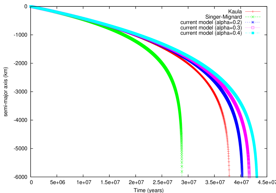
Figure 2:   Evolution of Phobos’ semi-major axis, as predicted by different models. The lines (from left to right) correspond to the Singer-Mignard model, to the Gerstenkorn-McDonald-Kaula model, and to the realistic rheology with $\,\alpha\,=\,0.2\,$, with $\,\alpha\,=\,0.3\,$, and with $\,\alpha\,=\,0.4\,$, correspondingly.

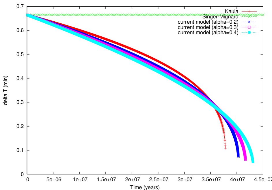
Figure 3:   Evolution of $\Delta t$ computed for three different models. The horizontal green line corresponds to the Singer-Mignard model wherein $\,\Delta t\,$ is set to be constant. The red line corresponds to the Gerstenkorn-MacDonald-Kaula model. The dark-blue, violet, and light-blue lines correspond to the realistic rheological models with $\,\alpha\,=\,0.2\;$, with $\,\alpha\,=\,0.3\,$. and with $\,\alpha\,=\,0.4\,$, correspondingly.

6 Conclusions

As the tidal angular lag $\,\delta\,$ is inversely proportional to the tidal $\,Q\,$ factor, the actual frequency-dependence of both $\,\delta\,$ and $\,\Delta t\,$ is unambiguously defined by the frequency-dependence of $\,Q\,$. While in the Gerstenkorn-MacDonald-Kaula theory of tides the geometric lag is assumed frequency-independent, in the Singer-Mignard theory it is the time lag that is spared of frequency dependence. However, neither of these two choices conform to the geophysical data.

We introduce a realistic tidal model, which permits the quality factor and, therefore, both the angular lag $\,\delta\,$ and the time lag $\,\Delta t\,$ to depend on the tidal frequency $\,\chi\,$. The quality factor is wont, according to numerous studies, to obey the law $\,Q\,\sim\,\chi^{\alpha}\,$, where $\,\alpha\,$ lies within $\,0.2\,-\,0.4\,$. This makes the time lag $\,\Delta t\,$ not a constant but a function (26) of the principal tidal frequency and, through (29), of the orbital elements of the satellite. The same pertains to the angular lag $\delta$.

Using these tidal-frequency dependencies for the time and angular lags, along with the recently updated values of the Martian parameters, we explored the future of Phobos, taking into account only the tides raised by Phobos on Mars, but not those caused by Mars on Phobos. Our integration shows that Phobos will fall on Mars in $\,40\,-\,43\,$ Myr from now. It is up to $\,50\,\%\,$ longer than the estimate stemming from the Singer-Mignard model employed in the past. This demonstrates that the currently accepted time scales of dynamical evolution, deduced from old tidal models, should be reexamined using the actual frequency dependence of the lags.

Acknowledgments
 
ME would like to deeply thank Peter Goldreich, Francis Nimmo, William Moore, and S. Fred Singer for their helpful comments and recommendations. VL wishes to gratefully acknowledge his fruitful conversation with Attilio Rivoldini concerning dissipation in Mars. The authors’ very special gratitude goes to Shun-ichiro Karato whose consultations on the theory and phenomenology of the quality factor were crucially important for the project.

Appendix.
 
The goal of this Appendix is threefold. First, we remind the reader why in the first approximation the quality factor is inversely proportional to the phase lag. Second, we explain why the phase lag is twice the geometric lag angle, as in formulae (8 - 9) above. While a comprehensive mathematical derivation of this fact can be found elsewhere (see the unnumbered formula between equations (29) and (30) on p. 673 in Kaula 1964), here we illustrate this counterintuitive result by using the simplest setting. Third, we justify our neglect of the first term in (20).  
 
A.1.  The case of a near-circular near-equatorial orbit.
 
Consider the simple case of an equatorial moon on a circular orbit. At each point of the planet, the tidal potential produced by this moon will read

$$W\;=\;W_{o}\;\cos\chi t\;\;\;,$$ (38)

the tidal frequency being given by

$$\chi\,=\,2~{}|n\;-\;\omega_{p}|~{}~{}~{}.~{}~{}~{}$$ (39)

Let  g  denote the free-fall acceleration. An element of the planet’s volume lying beneath the satellite’s trajectory will then experience a vertical elevation of

$$\zeta\;=\;\frac{W_{o}}{\mbox{g}}\;\cos(\chi t\;-\;2\delta)\;\;\;.$$ (40)

Accordingly, the vertical velocity of this element of the planet’s volume will amount to

$$u\;=\;\dot{\zeta}\;=\;-\;\chi\;\frac{W_{o}}{\mbox{g}}\;\sin(\chi t\;-\;2\;\delta)\;=\;-\;\chi\;\frac{W_{o}}{\mbox{g}}\;\left(\sin\chi t\;\cos 2\delta\;-\;\cos\chi t\;\sin 2\delta\right)\;\;.\;\;$$ (41)

The expression for the velocity has such a simple form because in this case the instantaneous frequency $\,\chi\,$ is constant. The satellite generates two bulges – on the facing and opposite sides of the planet – so each point of the surface is uplifted twice through a cycle. This entails the factor of two in the expressions (39) for the frequency. The phase in (40), too, is doubled, though the necessity of this is less evident.

The energy dissipated over a time cycle $\,T\,=\,2\pi/\chi\,$, per unit mass, will, in neglect of horizontal displacements, be

$$\Delta E_{{}_{cycle}} = \int^{T}_{0}u\left(-\,\frac{\partial W}{\partial r}\right)dt=\,-\left(-\,\chi\frac{W_{o}}{\mbox{g}}\right)\,\frac{\partial W_{o}}{\partial r}\int^{t=T}_{t=0}\cos\chi t\,\left(\sin\chi t\,\cos 2\delta\,-\,\cos\chi t\,\sin 2\delta\right)dt$$ (42)

$$= \,-\;\chi\;\frac{W_{o}}{\mbox{g}}\;\frac{\partial W_{o}}{\partial r}\;\sin 2\delta\;\frac{1}{\chi}\;\int^{\chi t\,=\,2\pi}_{\chi t\,=\,0}\;\cos^{2}\chi t\;\;d(\chi t)\;=\;-\;\frac{W_{o}}{\mbox{g}}\;\frac{\partial W_{o}}{\partial r}\;\pi\;\sin 2\delta\;\;,\;\;\;~{}~{}~{}~{}~{}~{}~{}~{}~{}~{}~{}~{}~{}~{}~{}~{}~{}~{}~{}~{}$$

while the peak energy stored in the system during the cycle will read:

$$E_{{}_{peak}} = \int^{T/4}_{0}u\left(-\,\frac{\partial W}{\partial r}\right)dt=\,-\left(-\,\chi\,\frac{W_{o}}{\mbox{g}}\right)\frac{\partial W_{o}}{\partial r}\int^{t=T/4}_{t=0}\cos\chi t\,\left(\sin\chi t\,\cos 2\delta\,-\,\cos\chi t\,\sin 2\delta\right)dt$$ (43)

$$= \;2\;\sigma\;\frac{W_{o}}{\mbox{g}}\;\frac{\partial W_{o}}{\partial r}\;\left[\;\frac{\cos 2\delta}{\chi}\;\int^{\chi t\,=\,\pi/2}_{\chi t\,=\,0}\;\cos\chi t\;\sin\chi t\;\;d(\chi t)\;-\;\frac{\sin 2\delta}{\chi}\;\int^{\chi t\,=\,\pi/2}_{\chi t\,=\,0}\;\cos^{2}\chi t\;\;d(\chi t)\;\right]$$

$$= \;\frac{W_{o}}{\mbox{g}}\;\frac{\partial W_{o}}{\partial r}\;\left[\;\frac{1}{2}\;\cos 2\delta\;-\;\frac{\pi}{4}\;\sin 2\delta\;\right]~{}~{}~{}~{}~{}~{}~{}~{}~{}~{}~{}~{}~{}~{}~{}~{}~{}~{}~{}~{}~{}~{}~{}~{}~{}~{}~{}~{}~{}~{}~{}~{}~{}~{}~{}~{}~{}~{}~{}~{}~{}~{}~{}~{}~{}~{}~{}~{}~{}~{}~{}~{}~{}~{}~{}~{}~{}~{}~{}~{}~{}~{}~{}~{}~{}~{}~{}~{}~{}~{}~{}~{}~{}~{}$$

whence

$$Q^{-1}\;=\;\frac{-\;\Delta E_{{}_{cycle}}}{2\,\pi\,E_{{}_{peak}}}\;=\;\frac{1}{2\,\pi}\;\,\frac{\pi\;\sin 2\delta}{~{}\frac{\textstyle 1}{\textstyle 2}\;\cos 2\delta\;-\;\frac{\textstyle\pi}{\textstyle 4}\;\sin 2\delta}\;\approx\;\tan 2\delta\;\;\;.$$ (44)

The above formulae were written down in neglect of horizontal displacements, approximation justified below in the language of continuum mechanics.  
 
A.2.  On the validity of our neglect of the horizontal displacements

In our above derivation of the interrelation between $\,Q\,$ and $\,\delta\,$, we greatly simplified the situation, taking into account only the vertical displacement of the planetary surface, in response to the satellite’s pull. Here we shall demonstrate that this approximation is legitimate, at least in the case when the planet is modeled with an incompressible and homogeneous medium.

As a starting point, recall that the tidal attenuation rate within a tidally distorted planet is well approximated with the work performed on it by the satellite:

$$\dot{E}\;=\;-\;\int\,\rho\;\mbox{{\boldmath$\vec{V}$}}\;\nabla W\;d^{3}x$$ (45)

where $\,\rho\,,\;\mbox{{\boldmath$\vec{V}$}}\,$ and $\,W\,$ are the density, velocity, and tidal potential inside the planet. To simplify this expression, we shall employ the equality

$$\rho\,\mbox{{\boldmath$\vec{V}$}}\,\nabla W\,=\,\nabla\,\cdot\,(\rho\;\mbox{{\boldmath$\vec{V}$}}\;W)\;-\;W\;\mbox{{\boldmath$\vec{V}$}}\cdot\nabla\rho\;-\;W\;\nabla\,\cdot\,(\rho\;\mbox{{\boldmath$\vec{V}$}})\,=\,\nabla\,\cdot\,(\rho\;\mbox{{\boldmath$\vec{V}$}}\;\nabla W)\;-\;W\;\mbox{{\boldmath$\vec{V}$}}\cdot\nabla\rho\;+\;W\;\frac{\partial\rho}{\partial t}\;\;.\;\;\;$$ (46)

For a homogeneous and incompressible primary, both the $\,\mbox{{\boldmath$\vec{V}$}}\;W\nabla\rho\,$ and $\,\partial\rho/\partial t\,$ terms are nil, wherefrom

$$\dot{E}\;=\;-\;\int\rho\;W\;\mbox{{\boldmath$\vec{V}$}}\,\cdot\,{\vec{\bf{n}}}\;d^{3}x\;\;\;,$$ (47)

${\vec{\bf{n}}}\,$ being the outward normal to the surface of the planet. We immediately see that, within the hydrodynamical model, it is only the radial elevation rate that matters.

Now write the potential as $\;W\,=\,W_{o}\,\cos(\chi\,t)\;$. Since the response is delayed by $\,\Delta t\,$, the surface-inequality rate will evolve as $\;\mbox{{\boldmath$\vec{V}$}}\cdot{\vec{\bf{n}}}\,\sim\,\sin\left[\,\chi\,(\,t\,-\,\Delta t\,)\,\right]\;$. All the rest will then be as in subsection A.1 above.

A.3.  On the validity of our neglect of the nondissipative tidal potential

The right-hand side of equation (32) consists of the principal part, $\;-\,{G\,(M_{o}\,+\,m)\,\mbox{{\boldmath$\vec{r}$}}}/{r^{3}}\,$, and tidal perturbation terms. These are the second and third terms from the right-hand side of (20), terms that bear a dependence on  $\vec{f}$  and, therefore, on $\,\Delta t\,$. The first term from the right-hand side of (20) lacks such a dependence and, therefore, is omitted in (32). The term was dropped because it would provide no secular input into the history of the semi-major axis. Here we shall provide a proof of this statement.

The omitted term corresponds to a potential (Mignard 1980):

$$U_{0}\;=\;\frac{k_{2}\;(M_{o}\,+\,m)\;G\;m\;R^{5}}{2\;M_{o}\;r^{6}}\;\;\;.$$ (48)

From the physical standpoint, $\,U_{0}\,$ models the effect of the tidal bulges, assuming their direction to coincide with that toward the tide-raising satellite. This potential entails no angular-momentum exchange, and therefore yields no secular effect on the semi-major axis. To prove this, let us decompose this potential into a series over the powers of $\,e\,$. This will require of us to derive the expression of $\,\left({\textstyle{a}}/{\textstyle{r}}\right)^{6}\,$. Starting out with the well known development

$$\frac{a}{r} = 1+\sum_{p=1}^{\infty}2J_{p}(pe)\cos(pM)$$ (49)

$$= 1+e\cos(M)+e^{2}\cos(2M)+\left(\frac{9}{8}\cos(3M)-\frac{1}{8}\cos(M)\right)e^{3}$$

$$+ \left(-\frac{1}{3}\cos(2M)+\frac{4}{3}\cos(4M)\right)e^{4}+\left(-\frac{81}{128}\cos(3M)+\frac{1}{192}\cos(M)+\frac{625}{384}\cos(5M)\right)e^{5}$$

$$+ \left(\frac{81}{40}\cos(6M)+\frac{1}{24}\cos(2M)-\frac{16}{15}\cos(4M)\right)e^{6}+...~{}~{}~{},~{}~{}~{}~{}~{}~{}~{}~{}~{}~{}~{}~{}~{}~{}~{}~{}~{}~{}~{}~{}~{}~{}~{}~{}~{}~{}~{}~{}~{}~{}~{}~{}~{}~{}~{}~{}~{}~{}~{}~{}~{}~{}~{}~{}~{}~{}~{}~{}~{}~{}~{}~{}$$

one can arrive to the following expansion:

$$\left(\frac{a}{r}\right)^{6} = 1+6e\cos(M)+\left(\frac{15}{2}+\frac{27}{2}\cos(2M)\right)e^{2}+\left(\frac{107}{4}\cos(3M)+\frac{117}{4}\cos(M)\right)e^{3}$$ (50)

$$+ \left(\frac{197}{4}\cos(4M)+\frac{101}{2}\cos(2M)+\frac{105}{4}\right)e^{4}$$

$$+ \left(\frac{5157}{64}\cos(3M)+\frac{5529}{64}\cos(5M)+\frac{2721}{32}\cos(M)\right)e^{5}$$

$$+ \left(\frac{4839}{40}\cos(4M)+129\cos(2M)+\frac{525}{8}+\frac{732}{5}\cos(6M)\right)e^{6}+...~{}~{}~{},$$

whose average over the mean anomaly looks like:

$$\langle\;\,\left(\frac{a}{r}\right)^{6}\;\rangle = 1+\frac{15}{2}e^{2}+\frac{105}{4}e^{4}+\frac{525}{8}e^{6}+...$$ (51)

Hence, the averaged potential will become:

$$\langle\,U_{0}\,\rangle=\frac{k_{2}(M_{0}+m)GmR^{5}}{2M_{0}a^{6}}\left(1+\frac{15}{2}e^{2}+\frac{105}{4}e^{4}+\frac{525}{8}e^{6}+...\right)$$ (52)

In the case of Phobos, the terms of order $\,O(e^{2})\,$ may, in the first approximation, be neglected. This means that out of the six Lagrange-type planetary equations the first five will, in the first order of $\,e\,$, stay unperturbed, and therefore the elements $\,a\,,\,e\,,\omega\,,\,{\it{i}}\,,\,\Omega\,$ will, in the first order over $\,e\,$, remain unchanged. The Lagrange equation for the longitude will be the only one influenced by $\,U_{0}\,$. That equation will assume the form:

$$\frac{dL}{dt}\;=\;n\;-\;\frac{2}{n\;a}\;\,\frac{\partial\;\langle\,U_{0}\,\rangle}{\partial\,a}$$ (53)

which gives

$$L\;=\;n\;t\;+\;\frac{6\;k_{2}\;(M_{o}\,+\,m)\;G\;m\;R^{5}}{M_{o}\;n\;a^{8}}\;t$$ (54)

We see that in the first order of $\,e\,$ the only secular effect stemming from the potential $\,U_{0}\,$ is a linear in time evolution of the longitude.

References

- [1] Bills, B. G., Neumann, G. A., Smith, D. E., & Zuber, M. T. 2005. “Improved estimate of tidal dissipation within Mars from MOLA observations of the shadow of Phobos.” Journal of Geophysical Research – Planets, Vol. 110, pp. 2376 - 2406. doi:10.1029/2004JE002376, 2005
- [2] Correia, A. C. M., & Laskar, J. 2003. “Different tidal torques on a planet with a dense atmosphere and consequences to the spin dynamics.” Journal of Geophysical Research – Planets, Vol. 108, pp. 5123 - 5132. doi:10.1029/2003JE002059, 2003
- [3] Darwin, G. H. 1908. “Tidal friction and cosmogony.” In: Darwin, G. H., Scientific Papers, Vol.2. Cambridge University Press, NY 1908.
- [4] Everhart, E. 1985. “An efficient integrator that uses Gauss-Radau spacings.” Dynamics of Comets: Their Origin and Evolution. Proceedings of IAU Colloquium 83 held in Rome on 11 - 15 June 1984. Edited by A. Carusi and G. B. Valsecchi. Dordrecht: Reidel, Astrophysics and Space Science Library. Vol. 115, p. 185 (1985)
-
[5]
Efroimsky, M. 2007. “Tidal torques. A critical review of some
techniques.”
Submitted to: Celestial Mechanics and Dynamical Astronomy.
arXiv:0712.1056 - [6] Flanagan, M. P., & Wiens, D. A. 1998. “Attenuation of broadband P and S waves in Tonga: Observations of frequency-dependent Q.” Pure and Applied Geophysics. Vol. 153, pp. 345 - 375. doi: 10.1007/s000240050199
- [7] Fontaine, F. R., Ildefonse, B., & Bagdassarov, N. 2005. “Temperature dependence of shear wave attenuation in partially molten gabbronorite at seismic frequencies.” Geophysical Journal International, Vol. 163, pp. 1025 - 1038
- [8] Gerstenkorn, H. 1955. “Über Gezeitenreibung beim Zweikörperproblem.” Zeitschrift für Astrophysik, Vol. 36, pp. 245 - 274
- [9] Goldreich, P. 1966. “History of the Lunar orbit.” Reviews of Geophysics, Vol. 4, pp. 411 - 439
- [10] Goldreich, P. 1963. “On the eccentricity of satellite orbits in the Solar system.” The Monthly Notes of the Royal Astronomical Society of London, Vol. 126, pp. 259 - 268.
- [11] Hanyk, L., Matyska, C., and Yuen, D. A., 1998. “Initial-value approach for viscoelastic responses of the Earth’s mantle.” In: Dynamics of the Ice Age Earth: A Modern Perspective, ed. by P. Wu. Trans Tech Publications Ltd, Zrich, Switzerland. pp. 135-154.
- [12] Hanyk, L., Matyska, C., and Yuen, D.A. 2000. “The problem of viscoelastic relaxation of the Earth solved by a matrix eigenvalue approach based on discretization in grid space.” Electronic Geosciences, Vol. 5, pp. 1 - 11.
- [13] Jeffreys, H. 1961. “The effect of tidal friction on eccentricity and inclination.” Monthly Notices of the Royal Astronomical Society of London Vol. 122, pp. 339 - 343
- [14] Jacobson, R., Synnott, S. P., and Campbell, J. K. C. 1989. “The orbits of the satellites of Mars from spacecraft and earthbased observations.” Astronomy & Astrophysics, Vol. 225, pp. 548 - 554
- [15] Karato, S.-i. 2007. Deformation of Earth Materials. An Introduction to the Rheology of Solid Earth. Cambridge University Press, UK. Chapter 11.
- [16] Karato, S.-i. 1998. “A Dislocation Model of Seismic Wave Attenuation and Micro-creep in the Earth: Harold Jeffreys and the Rheology of the Solid Earth.” Pure and Applied Geophysics. Vol. 153, No 2, pp. 239 - 256.
- [17] Karato, S.-i., and Spetzler, H. A. 1990. “Defect Microdynamics in Minerals and Solid-State Mechanisms of Seismic Wave Attenuation and Velocity Dispersion in the Mantle.” Reviews of Geophysics, Vol. 28, pp. 399 - 423
- [18] Kaula, W. M. 1964. “Tidal Dissipation by Solid Friction and the Resulting Orbital Evolution.” Reviews of Geophysics, Vol. 2, pp. 661 - 684
- [19] Lainey, V., Dehant, V., & Pätzold, M. 2007. “First numerical ephemerides of the Martian moons.” Astronomy & Astrophysics. Vol. 465, pp. 1075 - 1084
- [20] MacDonald, G. J. F. 1964. “Tidal Friction.” Reviews of Geophysics. Vol. 2, pp. 467 - 541
- [21] Mignard, F. 1979. “The Evolution of the Lunar Orbit Revisited. I.” The Moon and the Planets. Vol. 20, pp. 301 - 315.
- [22] Mignard, F. 1980. “The Evolution of the Lunar Orbit Revisited. II.” The Moon and the Planets. Vol. 23, pp. 185 - 201.
- [23] Mignard, F. 1981. “Evolution of the Martian satellites.” The Monthly Notices of the Royal Astronomical Society. Vol. 194, pp. 365 - 379.
- [24] Mitchell, B. J. 1995. “Anelastic structure and evolution of the continental crust and upper mantle from seismic surface wave attenuation.” Reviews of Geophysics, Vol. 33, No 4, pp. 441 - 462.
- [25] Mitrovica, J. X., and Peltier, W. R. 1992. “A comparison of methods for the inversion of viscoelastic relaxation spectra.” Geophysical Journal International, Vol. 108, pp. 410 - 414.
- [26] Moore, W., and Schubert, G. 2000. “The Tidal Response of Europa.” Icarus, Vol. 147, pp. 317 - 319.
- [27] Peale, S. J., and Cassen, P. 1978. “Contribution of Tidal Dissipation to Lunar Thermal History.” Icarus, Vol. 36, pp. 245 - 269
- [28] Peale, S. J., & Lee, M. H. 2000. “The Puzzle of the Titan-Hyperion 4:3 Orbital Resonance.” Talk at the DDA Meeting of the American Astronomical Society. Bulletin of the American Astronomical Society, Vol. 32, p. 860
-
[29]
Rainey, E. S. G., & Aharonson, O. 2006.
“Estimate of tidal Q of Mars using MOC observations of
the shadow of Phobos.” The 37th Annual Lunar and
Planetary Science Conference, 13 - 17 March 2006,
League City TX. Abstract No 2138.
http://www.lpi.usra.edu/meetings/lpsc2006/pdf/2138.pdf - [30] Shito, A., Karato, S.-i., & Park, J. 2004. “Frequency dependence of in Earth’s upper mantle, inferred from continuous spectra of body wave.” Geophysical Research Letters, Vol. 31, No 12, p. L12603, doi:10.1029/2004GL019582
- [31] Singer, S. F. 1968. “The Origin of the Moon and Geophysical Consequences.” The Geophysical Journal of the Royal Astronomical Society, Vol. 15, pp. 205 - 226.
- [32] Sokolnikoff, I. S. 1956. Mathematical Theory of Elasticity. 2nd Ed., McGraw-Hill NY 1956.
- [33] Stachnik, J. C., Abers, G. A., & Christensen, D. H. 2004. “Seismic attenuation and mantle wedge temperatures in the Alaska subduction zone.” Journal of Geophysical Research – Solid Earth, Vol. 109, No B10, p. B10304, doi:10.1029/2004JB003018
- [34] Tan, B. H., Jackson, I., & Fitz Gerald J. D. 1997. “Shear wave dispersion and attenuation in fine-grained synthetic olivine aggregates: preliminary results.” Geophysical Research Letters, Vol. 24, No 9, pp. 1055 - 1058, doi:10.1029/97GL00860
- [35] Williams, J. G., Boggs, D. H., Yoder, C. F., Ratcliff, J. T., and Dickey, J. O. 2001. “Lunar rotational dissipation in solid-body and molten core.” The Journal of Geophysical Research – Planets, Vol. 106, No E11, pp. 27933 - 27968. doi:10.1029/2000JE001396