Study of $e^{+}e^{-}\to\mathchar 28931\relax\kern 2.39996pt\overline{\kern-2.39996pt\mathchar 28931\relax\kern 0.60004pt}\kern-0.60004pt{},\;\mathchar 28931\relax\kern 2.39996pt\overline{\kern-2.39996pt\mathchar 28934\relax}{}^{0},\;\mathchar 28934\relax^{0}\kern 2.39996pt\overline{\kern-2.39996pt\mathchar 28934\relax}{}^{0}$ using Initial State Radiation with BABAR 

Abstract

We study the $e^{+}e^{-}\to\mathchar 28931\relax\kern 1.99997pt\overline{\kern-1.99997pt\mathchar 28931\relax\kern 0.50003pt}\kern-0.50003pt{}\gamma,\;\mathchar 28931\relax\kern 1.99997pt\overline{\kern-1.99997pt\mathchar 28934\relax}{}^{0}\gamma,\;\mathchar 28934\relax^{0}\kern 1.99997pt\overline{\kern-1.99997pt\mathchar 28934\relax}{}^{0}\gamma$ processes using 230 fb^-1 of integrated luminosity collected by the BABAR detector at $e^{+}e^{-}$ center-of-mass energy of 10.58 GeV. From the analysis of the baryon-antibaryon mass spectra the cross sections for $e^{+}e^{-}\to\mathchar 28931\relax\kern 1.99997pt\overline{\kern-1.99997pt\mathchar 28931\relax\kern 0.50003pt}\kern-0.50003pt{},\;\mathchar 28931\relax\kern 1.99997pt\overline{\kern-1.99997pt\mathchar 28934\relax}{}^{0},\;\mathchar 28934\relax^{0}\kern 1.99997pt\overline{\kern-1.99997pt\mathchar 28934\relax}{}^{0}$ are measured in the dibaryon mass range from threshold up to 3 GeV/$c^{2}$. The ratio of electric and magnetic form factors, $|G_{E}/G_{M}|$, is measured for $e^{+}e^{-}\to\mathchar 28931\relax\kern 1.99997pt\overline{\kern-1.99997pt\mathchar 28931\relax\kern 0.50003pt}\kern-0.50003pt{}$, and limits on the relative phase between $\mathchar 28931\relax$ form factors are obtained. We also measure the $J/\psi\to\mathchar 28931\relax\kern 1.99997pt\overline{\kern-1.99997pt\mathchar 28931\relax\kern 0.50003pt}\kern-0.50003pt{},\;\mathchar 28934\relax^{0}\kern 1.99997pt\overline{\kern-1.99997pt\mathchar 28934\relax}{}^{0}$ and $\psi(2S)\to\mathchar 28931\relax\kern 1.99997pt\overline{\kern-1.99997pt\mathchar 28931\relax\kern 0.50003pt}\kern-0.50003pt{}$ branching fractions.

I Introduction

In this paper we continue the experimental study of baryon time-like electromagnetic form factors. In our previous work BADpp we have measured the energy dependence of the cross section for $e^{+}e^{-}\to p\overline{p}$ and of the proton form factor using the initial state radiation (ISR) technique. Here we use this technique to study the processes $e^{+}e^{-}\to\mathchar 28931\relax\kern 1.99997pt\overline{\kern-1.99997pt\mathchar 28931\relax\kern 0.50003pt}\kern-0.50003pt{},\;\mathchar 28934\relax^{0}\kern 1.99997pt\overline{\kern-1.99997pt\mathchar 28934\relax}{}^{0},\;\mathchar 28931\relax\kern 1.99997pt\overline{\kern-1.99997pt\mathchar 28934\relax}{}^{0}$. The Born cross section for the ISR process $e^{+}e^{-}\to f+\gamma$ (Fig.1), where $f$ is a hadronic system, integrated over the hadron momenta, is given by

$$\frac{{\rm d}\sigma_{e^{+}e^{-}\to f\gamma}(m)}{{\rm d}m\,{\rm d}\cos{\theta_{\gamma}^{\ast}}}=\frac{2m}{s}\,W(x,\theta_{\gamma}^{\ast})\,\sigma_{f}(m),$$ (1)

where $\sqrt{s}$ is the $e^{+}e^{-}$ center-of-mass energy (c.m.), $m$ is the invariant mass of the hadronic system, $\sigma_{f}(m)$ is the cross section for $e^{+}e^{-}\to f$ reaction, $x\equiv{E_{\gamma}^{\ast}}/\sqrt{s}=1-{m^{2}}/{s}$, and $E_{\gamma}^{\ast}$ and $\theta_{\gamma}^{\ast}$ are the ISR photon energy and polar angle, respectively, in the $e^{+}e^{-}$ c.m. frame. The function BM

$$W(x,\theta_{\gamma}^{\ast})=\frac{\alpha}{\pi x}\left(\frac{2-2x+x^{2}}{\sin^{2}\theta_{\gamma}^{\ast}}-\frac{x^{2}}{2}\right)$$ (2)

describes the probability of ISR photon emission for $\theta_{\gamma}^{\ast}\gg m_{e}/\sqrt{s}$, where $\alpha$ is the fine structure constant and $m_{e}$ is the electron mass.

Figure 1: The Feynman diagram describing the ISR process $e^{+}e^{-}\to f\gamma$, where $f$ is a hadronic system.

The cross section for the process $e^{+}e^{-}\to B\kern 1.79993pt\overline{\kern-1.79993ptB}{}$, where $B$ is a spin-1/2 baryon, depends on magnetic ($G_{M}$) and electric ($G_{E}$) form factors as follows:

$$\sigma_{B\kern 1.25995pt\overline{\kern-1.25995ptB}{}}(m)=\frac{4\pi\alpha^{2}\beta}{3m^{2}}\left[|G_{M}(m)|^{2}+\frac{1}{2\tau}|G_{E}(m)|^{2}\right],$$ (3)

where $\beta=\sqrt{1-4m_{B}^{2}/m^{2}}$ and $\tau=m^{2}/4m_{B}^{2}$; at threshold, $G_{E}=G_{M}$. The cross section determines the linear combination of the squared form factors

$$|F(m)|^{2}=\frac{2\tau|G_{M}(m)|^{2}+|G_{E}(m)|^{2}}{2\tau+1},$$ (4)

and we define $|F(m)|$ to be the effective form factor BADpp .

The modulus of the ratio of electric and magnetic form factors can be determined from the analysis of the distribution of $\cos{\theta_{B}}$, where $\theta_{B}$ is the angle between the baryon momentum in the dibaryon rest frame and the momentum of the $B\kern 1.79993pt\overline{\kern-1.79993ptB}{}$ system in the $e^{+}e^{-}$ c.m. frame. This distribution can be expressed as the sum of the terms proportional $|G_{M}|^{2}$ and $|G_{E}|^{2}$. The $\theta_{B}$ dependencies of the $G_{E}$ and $G_{M}$ terms are close to $\sin^{2}\theta_{B}$ and $1+\cos^{2}\theta_{B}$ angular distributions for electric and magnetic form factors in the $e^{+}e^{-}\to B\kern 1.79993pt\overline{\kern-1.79993ptB}{}$ process. The full differential cross section for $e^{+}e^{-}\to B\kern 1.79993pt\overline{\kern-1.79993ptB}{}\gamma$ dkm is given in the Appendix.

A nonzero relative phase between the electric and magnetic form factors manifests itself in polarization of the outgoing baryons. In the $e^{+}e^{-}\to B\kern 1.79993pt\overline{\kern-1.79993ptB}{}$ reaction this polarization is perpendicular to the production plane dub . For the ISR process $e^{+}e^{-}\to B\kern 1.79993pt\overline{\kern-1.79993ptB}{}\gamma$ the polarization observables are analyzed in Refs. kuhn_ll ; dkm . The expression for the baryon polarization as a function of $G_{E}$, $G_{M}$, and momenta of the initial electron, ISR photon, and final baryon dkm is given in the Appendix. In the case of the $\mathchar 28931\relax\kern 1.99997pt\overline{\kern-1.99997pt\mathchar 28931\relax\kern 0.50003pt}\kern-0.50003pt{}$ final state the $\mathchar 28931\relax\to p\pi^{-}$ decay can be used to measure the $\mathchar 28931\relax$ polarization and hence the phase between the form factors.

Experimental information on the $e^{+}e^{-}\to\mathchar 28931\relax\kern 1.99997pt\overline{\kern-1.99997pt\mathchar 28931\relax\kern 0.50003pt}\kern-0.50003pt{}$, $\mathchar 28934\relax^{0}\kern 1.99997pt\overline{\kern-1.99997pt\mathchar 28934\relax}{}^{0}$, $\mathchar 28931\relax\kern 1.99997pt\overline{\kern-1.99997pt\mathchar 28934\relax}{}^{0}$ reactions is very scarce. The $e^{+}e^{-}\to\mathchar 28931\relax\kern 1.99997pt\overline{\kern-1.99997pt\mathchar 28931\relax\kern 0.50003pt}\kern-0.50003pt{}$ cross section is measured as $100^{+65}_{-35}$ pb at 2.386 GeV, and at the same energy upper limits for $e^{+}e^{-}\to\mathchar 28934\relax^{0}\kern 1.99997pt\overline{\kern-1.99997pt\mathchar 28934\relax}{}^{0}$ ($<120$ pb) and $e^{+}e^{-}\to\mathchar 28931\relax\kern 1.99997pt\overline{\kern-1.99997pt\mathchar 28934\relax}{}^{0}$ ($<75$ pb) cross sections have been obtained DM2ll . No other experimental results exist.

II The BABAR detector and data samples

We analyse a data sample corresponding to an integrated luminosity of 230 fb^-1 recorded with the BABAR detector babar-nim at the PEP-II asymmetric-energy storage rings. At PEP-II, 9-GeV electrons collide with 3.1-GeV positrons at a center-of-mass energy of 10.58 GeV (the $\mathchar 28935\relax$(4S) resonance). Additional data ($\sim 10\%$) recorded at 10.54 GeV are included in the present analysis.

Charged-particle tracking is provided by a five-layer silicon vertex tracker (SVT) and a 40-layer drift chamber (DCH), operating in a 1.5-T axial magnetic field. The transverse momentum resolution is 0.47% at 1 GeV/$c$. Energies of photons and electrons are measured with a CsI(Tl) electromagnetic calorimeter (EMC) with a resolution of 3% at 1 GeV. Charged-particle identification is provided by specific ionization (${\rm d}E/{\rm d}x$) measurements in the SVT and DCH, and by an internally reflecting ring-imaging Cherenkov detector (DIRC). Muons are identified in the solenoid’s instrumented flux return, which consists of iron plates interleaved with resistive plate chambers.

Signal ISR processes are simulated with the Monte Carlo (MC) event generator Phokhara phokhara ; kuhn_pp . Because the polar-angle distribution of the ISR photon is peaked near $0^{\circ}$ and $180^{\circ}$, the MC events are generated with a restriction on the photon polar angle: $20^{\circ}<\theta_{\gamma}^{\ast}<160^{\circ}$. The Phokhara event generator includes next-to-leading-order radiative corrections to the Born cross section. In particular, it generates an extra soft photon emitted from the initial state. To restrict the maximum energy of the extra photon we require that the invariant mass of the dibaryon system and the ISR photon satisfies $M_{B\kern 1.25995pt\overline{\kern-1.25995ptB}{}\gamma}>8$ GeV/$c^{2}$. The generated events are subjected to detailed detector simulation based on GEANT4 GEANT4 , and are reconstructed with the software chain used for the experimental data. Variations in the detector and in the beam background conditions are taken into account. For the full simulation we use the differential cross section for the $e^{+}e^{-}\to B\kern 1.79993pt\overline{\kern-1.79993ptB}{}\gamma$ process with $G_{E}=G_{M}$. In order to study angular distributions and model dependence of detection efficiency we produce two large samples of simulated events at the generator level, one with $G_{E}=0$ and the other with $G_{M}=0$, and reweight the events from the full simulation sample according to the desired $|G_{E}/G_{M}|$ ratio.

Background from $e^{+}e^{-}\to q\overline{q}$, where $q$ represents a $u$, $d$, $s$ or $c$ quark, is simulated with the JETSET JETSET event generator. JETSET also generates ISR events with hadron invariant mass above 2 GeV/$c^{2}$ and therefore can be used to study ISR background with baryons in the final state. The most important background processes $e^{+}e^{-}\to B\kern 1.79993pt\overline{\kern-1.79993ptB}{}\pi^{0}\gamma$, $e^{+}e^{-}\to B\kern 1.79993pt\overline{\kern-1.79993ptB}{}\pi^{0}$, and $e^{+}e^{-}\to\mathchar 28931\relax\overline{p}K^{+}\gamma$ are simulated separately. Three-body phase space and the Bonneau-Martin formula BM are used to generate the angular and energy distributions for the final hadrons and ISR photon, respectively. For these processes extra soft-photon radiation from the initial state is generated using the structure function method strfun .

III The reaction $e^{+}e^{-}\to\mathchar 28931\relax\kern 1.99997pt\overline{\kern-1.99997pt\mathchar 28931\relax\kern 0.50003pt}\kern-0.50003pt{}\gamma$

Figure 2: The $\chi^{2}_{\mathchar 28931\relax\mathchar 28931\relax}$ distributions for data (a) and $e^{+}e^{-}\to\mathchar 28931\relax\kern 1.99997pt\overline{\kern-1.99997pt\mathchar 28931\relax\kern 0.50003pt}\kern-0.50003pt{}\gamma$ simulation(b).

III.1 Event selection

The initial selection of events requires the presence of a high energy photon and at least one $\mathchar 28931\relax$ and one $\kern 1.99997pt\overline{\kern-1.99997pt\mathchar 28931\relax\kern 0.50003pt}\kern-0.50003pt{}$ candidate. The hard photon must have energy in the c.m. frame $E^{\ast}_{\gamma}>3$ GeV. The $\mathchar 28931\relax\to p\pi^{-}$ decay mode with the branching fraction of $(63.9\pm 0.5)\%$ pdg is used to identify $\mathchar 28931\relax$ candidates. Two oppositely-charged tracks are assigned the proton and pion mass hypotheses and fitted to a common vertex. Any combination with invariant mass in the range 1.104-1.128 GeV/$c^{2}$ (the nominal $\mathchar 28931\relax$ mass is 1.115683(6) GeV/$c^{2}$ pdg ), laboratory momentum greater than 0.5 GeV/$c$, and fit probability greater than 0.001 is considered a $\mathchar 28931\relax$ candidate. The candidate is then refitted with a $\mathchar 28931\relax$ mass constraint to improve the precision of the $\mathchar 28931\relax$ momentum measurement. To suppress combinatorial background we require that at least one of the proton candidates be identified as a proton according to the specific ionization (${\rm d}E/{\rm d}x$) measured in the SVT and DCH, and the Cherenkov angle measured in the DIRC.

For events passing the preliminary selection, we perform a kinematic fit that imposes energy and momentum conservation at the production vertex to the $\mathchar 28931\relax$ and $\kern 1.99997pt\overline{\kern-1.99997pt\mathchar 28931\relax\kern 0.50003pt}\kern-0.50003pt{}$ candidates and the photon with highest $E^{\ast}_{\gamma}$. For events with more than one $\mathchar 28931\relax$ ($\kern 1.99997pt\overline{\kern-1.99997pt\mathchar 28931\relax\kern 0.50003pt}\kern-0.50003pt{}$) candidate we consider all possible $\mathchar 28931\relax\kern 1.99997pt\overline{\kern-1.99997pt\mathchar 28931\relax\kern 0.50003pt}\kern-0.50003pt{}$ combinations, and the one giving the lowest $\chi^{2}$ for the kinematic fit is retained. The MC simulation does not accurately reproduce the shape of the resolution function for the photon energy. This leads to a difference in the $\chi^{2}$ distributions resulting from the kinematic fits to data and simulated events. To reduce this difference, only the measured direction of the ISR photon is used in the fit; its energy is a fit parameter.

Figure 3: Scatter plots of the invariant mass of the $\mathchar 28931\relax$ candidate versus the invariant mass of the $\kern 1.99997pt\overline{\kern-1.99997pt\mathchar 28931\relax\kern 0.50003pt}\kern-0.50003pt{}$ candidate for data (a) and $e^{+}e^{-}\to\mathchar 28931\relax\kern 1.99997pt\overline{\kern-1.99997pt\mathchar 28931\relax\kern 0.50003pt}\kern-0.50003pt{}\gamma$ simulation (b).

Figure 4: The $\mathchar 28931\relax\kern 1.99997pt\overline{\kern-1.99997pt\mathchar 28931\relax\kern 0.50003pt}\kern-0.50003pt{}$ mass spectrum for events satisfying the $\mathchar 28931\relax\kern 1.99997pt\overline{\kern-1.99997pt\mathchar 28931\relax\kern 0.50003pt}\kern-0.50003pt{}\gamma$ selection criteria.

The $\chi^{2}$ distributions for the kinematic fit ($\chi^{2}_{\mathchar 28931\relax\mathchar 28931\relax}$) to data events and to simulated $e^{+}e^{-}\to\mathchar 28931\relax\kern 1.99997pt\overline{\kern-1.99997pt\mathchar 28931\relax\kern 0.50003pt}\kern-0.50003pt{}\gamma$ events are shown in Fig. 2. We select the events with $\chi^{2}_{\mathchar 28931\relax\mathchar 28931\relax}<20$ for further analysis. The control region $20<\chi^{2}_{\mathchar 28931\relax\mathchar 28931\relax}<40$ is used for background estimation and subtraction.

Possible sources of background for the process under study are those with only one $\mathchar 28931\relax$ in the final state, such as $e^{+}e^{-}\to\mathchar 28931\relax\overline{p}K^{+}\gamma$. Such events contain a charged kaon instead of one of the pion candidates. To suppress this background we require that no charged pion candidate be identified as a kaon. This requirement rejects 70% of the background from $e^{+}e^{-}\to\mathchar 28931\relax\overline{p}K^{+}\gamma$ and only $\sim$2% of signal events.

The scatter plot of the invariant mass of the $\mathchar 28931\relax$ candidate versus the invariant mass of the $\kern 1.99997pt\overline{\kern-1.99997pt\mathchar 28931\relax\kern 0.50003pt}\kern-0.50003pt{}$ candidate for the 387 data events passing all the selection criteria is shown in Fig. 4(a) and that for simulated $e^{+}e^{-}\to\mathchar 28931\relax\kern 1.99997pt\overline{\kern-1.99997pt\mathchar 28931\relax\kern 0.50003pt}\kern-0.50003pt{}\gamma$ events is shown in Fig. 4(b). The $\mathchar 28931\relax\kern 1.99997pt\overline{\kern-1.99997pt\mathchar 28931\relax\kern 0.50003pt}\kern-0.50003pt{}$ invariant mass spectrum for data events is shown in Fig. 4. About half of the events have invariant mass below 3 GeV/$c^{2}$. Signals due to $J/\psi\to\mathchar 28931\relax\kern 1.99997pt\overline{\kern-1.99997pt\mathchar 28931\relax\kern 0.50003pt}\kern-0.50003pt{}$ and $\psi(2S)\to\mathchar 28931\relax\kern 1.99997pt\overline{\kern-1.99997pt\mathchar 28931\relax\kern 0.50003pt}\kern-0.50003pt{}$ decays are also clearly seen.

III.2 Background subtraction

Processes of three kinds potentially contribute background to the $e^{+}e^{-}\to\mathchar 28931\relax\kern 1.99997pt\overline{\kern-1.99997pt\mathchar 28931\relax\kern 0.50003pt}\kern-0.50003pt{}\gamma$ data sample, namely those with zero, one and two $\mathchar 28931\relax$’s in the final state.

The composition of the one-$\mathchar 28931\relax$ background is studied using JETSET simulation. This background is dominated by $e^{+}e^{-}\to\mathchar 28931\relax\overline{p}K^{+}\gamma$ events. Other processes also contain a charged kaon in the final state. The level of the one-$\mathchar 28931\relax$ background can be estimated from the fraction of data events rejected by the requirement that no $\pi^{+}$ candidate be identified as a $K^{+}$. For $M_{\mathchar 28931\relax\kern 1.39998pt\overline{\kern-1.39998pt\mathchar 28931\relax\kern 0.35002pt}\kern-0.35002pt{}}<3$ GeV/$c^{2}$ this fraction is 3/224, and we estimate that the one-$\mathchar 28931\relax$ background does not exceed 1.6 events at 90% confidence level (CL).

Figure 5: The values of $S_{i}$ (see text) obtained from fits to data (points with error bars) and from fits to $e^{+}e^{-}\to\mathchar 28931\relax\kern 1.99997pt\overline{\kern-1.99997pt\mathchar 28931\relax\kern 0.50003pt}\kern-0.50003pt{}\gamma$ simulated events (histogram).

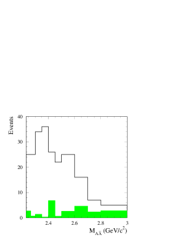
Figure 6: The distribution of data events satisfying the $\mathchar 28931\relax\kern 1.99997pt\overline{\kern-1.99997pt\mathchar 28931\relax\kern 0.50003pt}\kern-0.50003pt{}\gamma$ selection criteria over chosen mass intervals. The shaded histogram shows fitted background.

A more precise estimation (but based on JETSET prediction for the composition of one-$\mathchar 28931\relax$ events) of this background is obtained using a special selection of $e^{+}e^{-}\to\mathchar 28931\relax\overline{p}K^{+}\gamma$ events. We select events with at least 4 charged tracks and a photon with $E_{\gamma}^{\ast}>3$ GeV. Two tracks, one of which is identified as a proton, must be combined to form a $\mathchar 28931\relax$ candidate, and the other two must originate from the $e^{+}e^{-}$ interaction point and be identified as an antiproton and a positively-charged kaon. For these events we perform the kinematic fit to the $e^{+}e^{-}\to\mathchar 28931\relax\overline{p}K^{+}\gamma$ hypothesis and require $\chi^{2}<20$. The background for $e^{+}e^{-}\to\mathchar 28931\relax\overline{p}K^{+}\gamma$ is estimated from the region $20<\chi^{2}<40$. The total number of selected $\mathchar 28931\relax\overline{p}K^{+}\gamma$ events is found to be $568\pm 30$. Using the ratio of detection efficiencies for $\mathchar 28931\relax\kern 1.99997pt\overline{\kern-1.99997pt\mathchar 28931\relax\kern 0.50003pt}\kern-0.50003pt{}\gamma$ and $\mathchar 28931\relax\overline{p}K^{+}\gamma$ selections obtained from simulation, $(0.12\pm 0.07)$%, we calculate the number of $\mathchar 28931\relax\overline{p}K^{+}\gamma$ events satisfying the $\mathchar 28931\relax\kern 1.99997pt\overline{\kern-1.99997pt\mathchar 28931\relax\kern 0.50003pt}\kern-0.50003pt{}\gamma$ selection criteria to be $0.7\pm 0.4$. Taking the ratio of $\mathchar 28931\relax\overline{p}K^{+}\gamma$ to all one-$\mathchar 28931\relax$ events (0.7) from JETSET simulation we estimate the total number of one-$\mathchar 28931\relax$ background events to be $1.0\pm 0.6$. The $e^{+}e^{-}\to\mathchar 28931\relax\overline{p}K^{+}\gamma$ simulation is reweighted to reproduce the shape of the experimental $M_{\mathchar 28931\relax pK}$ distribution. The reweighted events are then used to find the distribution of $M_{\mathchar 28931\relax\kern 1.39998pt\overline{\kern-1.39998pt\mathchar 28931\relax\kern 0.35002pt}\kern-0.35002pt{}}$ for events with only one real $\mathchar 28931\relax$. We estimate $0.8\pm 0.5$ background events to have $M_{\mathchar 28931\relax\kern 1.39998pt\overline{\kern-1.39998pt\mathchar 28931\relax\kern 0.35002pt}\kern-0.35002pt{}}<3$ GeV/$c^{2}$.

The background processes with no real $\mathchar 28931\relax$’s are ISR processes with four charged particles in the final state: $e^{+}e^{-}\to 2\pi^{+}2\pi^{-}\gamma$, $K^{+}K^{-}\pi^{+}\pi^{-}\gamma$, $K^{+}K_{S}\pi^{-}\gamma$, $p\overline{p}\pi^{+}\pi^{-}\gamma$, $2\pi^{+}2\pi^{-}\pi^{0}$, etc. The background from these processes can be estimated from an analysis of the two-dimensional distribution of the $\mathchar 28931\relax$ and $\kern 1.99997pt\overline{\kern-1.99997pt\mathchar 28931\relax\kern 0.50003pt}\kern-0.50003pt{}$ candidate mass values. The $6\times 6$ two-dimensional histogram corresponding to the plot in Fig. 4a is fitted by the following function:

$$n_{ij}=N_{2}S_{i}S_{j}+N_{0}B_{0i}B_{0j}+N_{1}(S_{i}B_{1j}+S_{j}B_{1i})/2.$$ (5)

where the six mass intervals are those shown in Fig. 5. Here $N_{2}$, $N_{1}$, and $N_{0}$ represent the numbers of events with two, one, and zero $\mathchar 28931\relax$’s, respectively; $N_{2}$ and $N_{0}$ are free fit parameters, and $N_{1}$ is fixed at the value determined above ($0.8\pm 0.5$ events for $M_{\mathchar 28931\relax\kern 1.39998pt\overline{\kern-1.39998pt\mathchar 28931\relax\kern 0.35002pt}\kern-0.35002pt{}}<3$ GeV/$c^{2}$); $S_{i}$ is the probability for a $\mathchar 28931\relax$ to have reconstructed mass in the $i$th mass bin, while $B_{0i}$ and $B_{1i}$ are the probabilities for a false $\mathchar 28931\relax$ candidate from background with zero and one real $\mathchar 28931\relax$, respectively. Since the one-$\mathchar 28931\relax$ background is small and its presence leads to only small changes in the fitted $N_{2}$ and $N_{0}$ values, we use a uniform distribution for $B_{1}(m)$, i.e. all $B_{1i}=1/6$. The $B_{0}(m)$ are parametrized by the linear function $B_{0i}=1/6+(i-3.5)\Delta$, and five of the $S_{i}$ and $\Delta$ are free fit parameters. For 221 events with $M_{\mathchar 28931\relax\kern 1.39998pt\overline{\kern-1.39998pt\mathchar 28931\relax\kern 0.35002pt}\kern-0.35002pt{}}<3$ GeV/$c^{2}$ the fit yields $N_{2}=216\pm 15$ and $N_{0}=4^{+4}_{-3}$. The fitted values of the $S_{i}$ are in good agreement with the values expected from $e^{+}e^{-}\to\mathchar 28931\relax\kern 1.99997pt\overline{\kern-1.99997pt\mathchar 28931\relax\kern 0.50003pt}\kern-0.50003pt{}\gamma$ simulation (Fig. 5). In particular, $S_{3}+S_{4}=0.950\pm 0.014$ for data and $0.953\pm 0.003$ for simulation.

The sources of two-$\mathchar 28931\relax$ background are processes with extra neutral particle(s) in the final state: $e^{+}e^{-}\to\mathchar 28931\relax\kern 1.99997pt\overline{\kern-1.99997pt\mathchar 28931\relax\kern 0.50003pt}\kern-0.50003pt{}\pi^{0}$, $e^{+}e^{-}\to\mathchar 28931\relax\kern 1.99997pt\overline{\kern-1.99997pt\mathchar 28931\relax\kern 0.50003pt}\kern-0.50003pt{}\gamma\gamma$, $e^{+}e^{-}\to\mathchar 28931\relax\kern 1.99997pt\overline{\kern-1.99997pt\mathchar 28931\relax\kern 0.50003pt}\kern-0.50003pt{}\pi^{0}\gamma$, etc. A significant fraction of $e^{+}e^{-}\to\mathchar 28931\relax\kern 1.99997pt\overline{\kern-1.99997pt\mathchar 28931\relax\kern 0.50003pt}\kern-0.50003pt{}\pi^{0}$ events with an undetected low-energy photon or with merged photons from $\pi^{0}$ decay are reconstructed under the $\mathchar 28931\relax\kern 1.99997pt\overline{\kern-1.99997pt\mathchar 28931\relax\kern 0.50003pt}\kern-0.50003pt{}\gamma$ hypothesis with a low value of $\chi^{2}_{\mathchar 28931\relax\mathchar 28931\relax}$, and can not be separated from the process under study. This background is studied by selecting a special subsample of events containing a $\mathchar 28931\relax$ and a $\kern 1.99997pt\overline{\kern-1.99997pt\mathchar 28931\relax\kern 0.50003pt}\kern-0.50003pt{}$ candidate and at least two photons, one with energy greater than 0.1 GeV and the other with c.m. energy above 3 GeV. The two-photon invariant mass is required to be in the range 0.07 to 0.2 GeV/$c^{2}$. A kinematic fit to the $e^{+}e^{-}\to\mathchar 28931\relax\kern 1.99997pt\overline{\kern-1.99997pt\mathchar 28931\relax\kern 0.50003pt}\kern-0.50003pt{}\gamma\gamma$ hypothesis is then performed. Requirements on the $\chi^{2}$ ($\chi^{2}<20$) and the two-photon invariant mass ($0.11<M_{\gamma\gamma}<0.16$ GeV/$c^{2}$) are imposed to define $\mathchar 28931\relax\kern 1.99997pt\overline{\kern-1.99997pt\mathchar 28931\relax\kern 0.50003pt}\kern-0.50003pt{}\pi^{0}$ candidates. No data events satisfy these criteria, and the expected background from $e^{+}e^{-}\to\mathchar 28931\relax\kern 1.99997pt\overline{\kern-1.99997pt\mathchar 28931\relax\kern 0.50003pt}\kern-0.50003pt{}\gamma$ is $0.8\pm 0.3$ events. The corresponding 90% CL upper limit on the number of selected $\mathchar 28931\relax\kern 1.99997pt\overline{\kern-1.99997pt\mathchar 28931\relax\kern 0.50003pt}\kern-0.50003pt{}\pi^{0}$ candidates is 1.6 events. Using the ratio of detection efficiencies for $\mathchar 28931\relax\kern 1.99997pt\overline{\kern-1.99997pt\mathchar 28931\relax\kern 0.50003pt}\kern-0.50003pt{}\pi^{0}$ and $\mathchar 28931\relax\kern 1.99997pt\overline{\kern-1.99997pt\mathchar 28931\relax\kern 0.50003pt}\kern-0.50003pt{}\gamma$ selections ($0.28\pm 0.02$) we find that the $\mathchar 28931\relax\kern 1.99997pt\overline{\kern-1.99997pt\mathchar 28931\relax\kern 0.50003pt}\kern-0.50003pt{}\pi^{0}$ background in $\mathchar 28931\relax\kern 1.99997pt\overline{\kern-1.99997pt\mathchar 28931\relax\kern 0.50003pt}\kern-0.50003pt{}\gamma$ sample does not exceed 6 events. This upper limit is used as a measure of the systematic uncertainty due to $\mathchar 28931\relax\kern 1.99997pt\overline{\kern-1.99997pt\mathchar 28931\relax\kern 0.50003pt}\kern-0.50003pt{}\pi^{0}$ background. We assume that the dibaryon mass spectrum in the $e^{+}e^{-}\to\mathchar 28931\relax\kern 1.99997pt\overline{\kern-1.99997pt\mathchar 28931\relax\kern 0.50003pt}\kern-0.50003pt{}\pi^{0}$ process is similar to that for the $p\overline{p}\pi^{0}$ final state BADpp . In particular, about 70% of $\mathchar 28931\relax\kern 1.99997pt\overline{\kern-1.99997pt\mathchar 28931\relax\kern 0.50003pt}\kern-0.50003pt{}\pi^{0}$ events are located in the $\mathchar 28931\relax\kern 1.99997pt\overline{\kern-1.99997pt\mathchar 28931\relax\kern 0.50003pt}\kern-0.50003pt{}$ mass region below 3 GeV/$c^{2}$. For this mass range this background does not exceed 2% of the selected $\mathchar 28931\relax\kern 1.99997pt\overline{\kern-1.99997pt\mathchar 28931\relax\kern 0.50003pt}\kern-0.50003pt{}\gamma$ candidates.

Table 1: The $\beta_{i}$ values obtained from simulation for signal and background processes, where $\beta_{i}$ is the ratio of the number of selected $\mathchar 28931\relax\kern 1.99997pt\overline{\kern-1.99997pt\mathchar 28931\relax\kern 0.50003pt}\kern-0.50003pt{}\gamma$ candidates with $20<\chi^{2}_{\mathchar 28931\relax\mathchar 28931\relax}<40$ to that with $\chi^{2}_{\mathchar 28931\relax\mathchar 28931\relax}<20$.

	$\mathchar 28931\relax\kern 1.99997pt\overline{\kern-1.99997pt\mathchar 28931\relax\kern 0.50003pt}\kern-0.50003pt{}\gamma$	$\mathchar 28931\relax\kern 1.99997pt\overline{\kern-1.99997pt\mathchar 28934\relax}{}^{0}\gamma$	$\mathchar 28934\relax^{0}\kern 1.99997pt\overline{\kern-1.99997pt\mathchar 28934\relax}{}^{0}\gamma$	$\mathchar 28931\relax\kern 1.99997pt\overline{\kern-1.99997pt\mathchar 28934\relax}{}^{0}\pi^{0}$	JETSET
$\beta_{i}$	$0.073\pm 0.005$	$0.83\pm 0.07$	$1.1\pm 0.2$	$0.81\pm 0.09$	$0.86\pm 0.06$

Table 2: $N$ is the number of selected $\mathchar 28931\relax\kern 1.99997pt\overline{\kern-1.99997pt\mathchar 28931\relax\kern 0.50003pt}\kern-0.50003pt{}\gamma$ candidates with $M_{\mathchar 28931\relax\kern 1.39998pt\overline{\kern-1.39998pt\mathchar 28931\relax\kern 0.35002pt}\kern-0.35002pt{}}<3$ GeV/$c^{2}$, $N_{2s}$ is the number of signal events, $N_{0}$, $N_{1}$, $N_{2b}$ indicate the number of background events with zero, one, and two $\mathchar 28931\relax$’s in the final state, respectively, and $N_{\mathchar 28931\relax\kern 1.39998pt\overline{\kern-1.39998pt\mathchar 28931\relax\kern 0.35002pt}\kern-0.35002pt{}\pi^{0}}$ is background from $e^{+}e^{-}\to\mathchar 28931\relax\kern 1.99997pt\overline{\kern-1.99997pt\mathchar 28931\relax\kern 0.50003pt}\kern-0.50003pt{}\pi^{0}$.

	$N$	$N_{2s}$	$N_{0}$	$N_{1}$	$N_{2b}$	$N_{\mathchar 28931\relax\kern 1.39998pt\overline{\kern-1.39998pt\mathchar 28931\relax\kern 0.35002pt}\kern-0.35002pt{}\pi^{0}}$
$\chi^{2}_{\mathchar 28931\relax\mathchar 28931\relax}<20$	221	$204\pm 19$	$4^{+4}_{-3}$	$0.8\pm 0.5$	$12\pm 10$	$<4$
$20<\chi^{2}_{\mathchar 28931\relax\mathchar 28931\relax}<40$	35	$15\pm 3$	$9^{+7}_{-5}$	$0.6\pm 0.4$	$11\pm 8$	$<1$
$\chi^{2}_{\mathchar 28931\relax\mathchar 28931\relax}<20$ (JETSET)	522	$500\pm 17$	$2.5\pm 1.2$	$0.6\pm 0.6$	$18\pm 3$	$1.2\pm 0.9$

The two-$\mathchar 28931\relax$ background other than from $e^{+}e^{-}\to\mathchar 28931\relax\kern 1.99997pt\overline{\kern-1.99997pt\mathchar 28931\relax\kern 0.50003pt}\kern-0.50003pt{}\pi^{0}$ has the $\chi^{2}_{\mathchar 28931\relax\mathchar 28931\relax}$ distribution very different from that for the process under study. Table 1 shows the ratio of numbers of selected $\mathchar 28931\relax\kern 1.99997pt\overline{\kern-1.99997pt\mathchar 28931\relax\kern 0.50003pt}\kern-0.50003pt{}\gamma$ candidates with $20<\chi^{2}_{\mathchar 28931\relax\mathchar 28931\relax}<40$ and $\chi^{2}_{\mathchar 28931\relax\mathchar 28931\relax}<20$ for signal and background processes. The ratios are obtained from simulation. The column denoted “JETSET” shows the result of JETSET simulation for background events containing two $\mathchar 28931\relax$’s in the final state. From the number of selected two-$\mathchar 28931\relax$ events in the signal and control $\chi^{2}_{\mathchar 28931\relax\mathchar 28931\relax}$ regions, $N_{2}(\chi^{2}<20)$ and $N_{2}(20<\chi^{2}<40)$, the numbers of signal and background events with $\chi^{2}_{\mathchar 28931\relax\mathchar 28931\relax}<20$ can be calculated as:

$$N_{2s} = \frac{N_{2}(\chi^{2}<20)-N_{2}(20<\chi^{2}<40)/\beta_{bkg}}{1-\beta_{sig}/\beta_{bkg}},$$

$$N_{2b} = N_{2}(\chi^{2}<20)-N_{2s},$$ (6)

where $\beta_{bkg}$ is the ratio of fractions of events in the control and signal $\chi^{2}$ regions averaged over all processes contributing into two-$\mathchar 28931\relax$ background. For this coefficient we use $\beta_{bkg}=0.9\pm 0.3$ which is close to the value obtained from the JETSET simulation, with an uncertainty covering the $\beta_{i}$ variations for different background processes. For the ratio for the signal process $\beta_{sig}$, we use the value obtained from simulation $\beta_{sig}=0.073\pm 0.010$. The quoted error takes into account MC statistics, the data-MC simulation difference in $\chi^{2}$ distribution, and the $\beta_{sig}$ variation as a function of $\mathchar 28931\relax\kern 1.99997pt\overline{\kern-1.99997pt\mathchar 28931\relax\kern 0.50003pt}\kern-0.50003pt{}$ mass. The difference between data and simulated $\chi^{2}$ distributions was studied in Ref. BADpp using the process $e^{+}e^{-}\to\mu^{+}\mu^{-}\gamma$. The resulting values of $N_{2s}$ and $N_{2b}$ for $\mathchar 28931\relax\kern 1.99997pt\overline{\kern-1.99997pt\mathchar 28931\relax\kern 0.50003pt}\kern-0.50003pt{}$ masses below 3 GeV/$c^{2}$ are listed in Table 2. The total background in the signal $\chi^{2}$ region from the processes with zero, one, and two $\mathchar 28931\relax$’s in final state is about 10%. The last row of the table shows the JETSET prediction for signal and background events in the signal $\chi^{2}$ region. The simulation overestimates the signal yield, but can be used for qualitative estimation of background level.

The procedure for background estimation and subtraction described above is applied in each of the twelve $\mathchar 28931\relax\kern 1.99997pt\overline{\kern-1.99997pt\mathchar 28931\relax\kern 0.50003pt}\kern-0.50003pt{}$ mass intervals indicated in Table 4. Due to restricted statistics we fit the two-dimensional histogram of $M_{p\pi^{-}}$ vs $M_{\overline{p}\pi^{+}}$ using $3\times 3$ bins, and fix the $S_{i}$ (see Eq.(5)) at the values obtained from MC simulation. The histograms for signal and control $\chi^{2}$ regions are fitted simultaneously. The free fit parameters are $N_{0}$ and $\Delta$ for the two $\chi^{2}$ regions, $N_{2s}$, and $N_{2b}$. Fig. 6 shows the distribution of selected events over the chosen mass intervals. The shaded histogram shows the background contribution obtained from the fit. The resulting numbers of signal events are listed in Table 4, where the quoted errors include the statistical errors and errors due to uncertainties in the $\beta_{sig}$, $\beta_{bkg}$ and $S_{i}$ coefficients. These coefficients are varied within their uncertainties during fitting. For the mass ranges $3.2<M_{\mathchar 28931\relax\kern 1.39998pt\overline{\kern-1.39998pt\mathchar 28931\relax\kern 0.35002pt}\kern-0.35002pt{}}<3.6$ GeV/$c^{2}$ and $3.8<M_{\mathchar 28931\relax\kern 1.39998pt\overline{\kern-1.39998pt\mathchar 28931\relax\kern 0.35002pt}\kern-0.35002pt{}}<5.0$ GeV/$c^{2}$ where we do not see evidence for a signal above background, 90% CL upper limits on the number of signal events are listed. The mass regions near the $J/\psi$ and $\psi(2S)$ will be considered separately in Sec. III.6.

III.3 Angular distributions for $e^{+}e^{-}\to\mathchar 28931\relax\kern 1.99997pt\overline{\kern-1.99997pt\mathchar 28931\relax\kern 0.50003pt}\kern-0.50003pt{}\gamma$

The modulus of the ratio of the electric and magnetic form factors can be extracted from an analysis of the distribution of $\cos{\theta_{\mathchar 28931\relax}}$, where $\theta_{\mathchar 28931\relax}$ is the angle between the $\mathchar 28931\relax$ momentum in the $\mathchar 28931\relax\kern 1.99997pt\overline{\kern-1.99997pt\mathchar 28931\relax\kern 0.50003pt}\kern-0.50003pt{}$ rest frame and the momentum of the $\mathchar 28931\relax\kern 1.99997pt\overline{\kern-1.99997pt\mathchar 28931\relax\kern 0.50003pt}\kern-0.50003pt{}$ system in the $e^{+}e^{-}$ c.m. frame. This distribution is given by

$$\frac{{\rm d}N}{{\rm d}\cos{\theta_{\mathchar 28931\relax}}} = A\,[\rule{0.0pt}{14.22636pt}H_{M}(\cos{\theta_{\mathchar 28931\relax}},M_{\mathchar 28931\relax\kern 1.39998pt\overline{\kern-1.39998pt\mathchar 28931\relax\kern 0.35002pt}\kern-0.35002pt{}})$$ (7)

$$+ \left|\frac{G_{E}}{G_{M}}\right|^{2}H_{E}(\cos{\theta_{\mathchar 28931\relax}},M_{\mathchar 28931\relax\kern 1.39998pt\overline{\kern-1.39998pt\mathchar 28931\relax\kern 0.35002pt}\kern-0.35002pt{}})].$$

The functions $H_{M}(\cos{\theta_{\mathchar 28931\relax}},M_{\mathchar 28931\relax\kern 1.39998pt\overline{\kern-1.39998pt\mathchar 28931\relax\kern 0.35002pt}\kern-0.35002pt{}})$ and $H_{E}(\cos{\theta_{\mathchar 28931\relax}},M_{\mathchar 28931\relax\kern 1.39998pt\overline{\kern-1.39998pt\mathchar 28931\relax\kern 0.35002pt}\kern-0.35002pt{}})$ do not have an analytic form, and so are calculated using MC simulation. To do this two samples of $e^{+}e^{-}\to\mathchar 28931\relax\kern 1.99997pt\overline{\kern-1.99997pt\mathchar 28931\relax\kern 0.50003pt}\kern-0.50003pt{}\gamma$ events were generated, one with $G_{E}=0$ and the other with $G_{M}=0$, using generator level simulation. The angular dependencies of the resulting functions do not differ significantly from the $(1+\cos^{2}\theta_{\mathchar 28931\relax})$ and $\sin^{2}\theta_{\mathchar 28931\relax}$ functions corresponding to the magnetic and electric form factors in the case of $e^{+}e^{-}\to\mathchar 28931\relax\kern 1.99997pt\overline{\kern-1.99997pt\mathchar 28931\relax\kern 0.50003pt}\kern-0.50003pt{}$.

The observed angular distributions are fitted in two mass intervals: from $\mathchar 28931\relax\kern 1.99997pt\overline{\kern-1.99997pt\mathchar 28931\relax\kern 0.50003pt}\kern-0.50003pt{}$ threshold to 2.4 GeV/$c^{2}$ and from 2.4 GeV/$c^{2}$ to 2.8 GeV/$c^{2}$. For each mass and angular interval, the background is subtracted by means of the procedure described in the previous section. The angular distributions obtained are shown in Fig. 7.

Figure 7: The $\cos{\theta_{\mathchar 28931\relax}}$ distribution for the mass regions 2.23–2.40 GeV/$c^{2}$ (a), and 2.40–2.80 GeV/$c^{2}$ (b). The points with error bars represent the data after background subtraction. The histograms are fit results: the dashed histogram shows the contributions corresponding to the magnetic form factor; the dotted histogram shows the contribution from the electric form factor, and the solid histogram is the sum of these two.

Figure 8: The $\cos{\theta_{\mathchar 28931\relax}}$ dependence of the detection efficiency for simulated events with $M_{\mathchar 28931\relax\kern 1.39998pt\overline{\kern-1.39998pt\mathchar 28931\relax\kern 0.35002pt}\kern-0.35002pt{}}<2.8$ GeV/$c^{2}$.

Figure 9: The $\cos{\theta_{\mathchar 28931\relax}}$ distributions for data (points with error bars) and simulation (histogram) corresponding to the reaction $e^{+}e^{-}\to J/\psi\gamma\to\mathchar 28931\relax\kern 1.99997pt\overline{\kern-1.99997pt\mathchar 28931\relax\kern 0.50003pt}\kern-0.50003pt{}\gamma$.

The distributions are fitted using the expression on the right-hand side of Eq. (7) with two free parameters $A$ and $|G_{E}/G_{M}|$. The functions $H_{M}$ and $H_{E}$ are replaced by the histograms, obtained from MC simulation with the $\mathchar 28931\relax\kern 1.99997pt\overline{\kern-1.99997pt\mathchar 28931\relax\kern 0.50003pt}\kern-0.50003pt{}$ selection criteria applied. To take into account the effect of these criteria (Fig. 8), the simulated events produced assuming $G_{E}=G_{M}$ are reweighted according to the $\cos{\theta_{\mathchar 28931\relax}}$ distributions obtained at generator level. These weight functions also take account of the difference in $\mathchar 28931\relax\kern 1.99997pt\overline{\kern-1.99997pt\mathchar 28931\relax\kern 0.50003pt}\kern-0.50003pt{}$ mass dependence between data and MC simulation. The histograms fitted to the angular distributions are shown in Fig. 7. The following values of the $|G_{E}/G_{M}|$ ratio are obtained:

$$|G_{E}/G_{M}|=1.73^{+0.99}_{-0.57}\;\;\mbox{ (2.23--2.40 GeV)}/c^{2},$$

$$|G_{E}/G_{M}|=0.71^{+0.66}_{-0.71}\;\;\mbox{ (2.40--2.80 GeV)}/c^{2}.$$

The quoted errors include both statistical and systematic uncertainties. The net systematic uncertainty does not exceed 15% of the statistical error and includes the uncertainties due to background subtraction, limited MC statistics, and the mass dependence of the $|G_{E}/G_{M}|$ ratio.

We also measure the angular distribution for $J/\psi\to\mathchar 28931\relax\kern 1.99997pt\overline{\kern-1.99997pt\mathchar 28931\relax\kern 0.50003pt}\kern-0.50003pt{}$ decay, for which the shape is usually described by the form $(1+\alpha\cos^{2}{\theta})$. The world average value of $\alpha=0.65\pm 0.10$ MARKll ; DM2psi ; BESll . The distribution for $J/\psi\to\mathchar 28931\relax\kern 1.99997pt\overline{\kern-1.99997pt\mathchar 28931\relax\kern 0.50003pt}\kern-0.50003pt{}$ decay in the present experiment is shown in Fig. 9. To remove background, this distribution was obtained as the difference between the histogram for the signal mass region (3.05-3.15 GeV/$c^{2}$) and that for the mass sidebands (3.00–3.05 and 3.15–3.20 GeV/$c^{2}$). The data distribution is in good agreement with that obtained from simulation with $\alpha=0.65$.

Our results on the $|G_{E}/G_{M}|$ ratio are consistent both with $|G_{E}/G_{M}|=1$, valid at the $\mathchar 28931\relax\kern 1.99997pt\overline{\kern-1.99997pt\mathchar 28931\relax\kern 0.50003pt}\kern-0.50003pt{}$ threshold, and with our results for the reaction $e^{+}e^{-}\to p\overline{p}$ for which this ratio was found to be greater than unity near threshold BADpp . The strong dependence of the $|G_{E}/G_{M}|$ ratio on the dibaryon mass near threshold is expected due to the baryon-antibaryon final state interaction FSI1 ; FSI2 .

III.4 Mass dependence of the detection efficiency

Figure 10: The $\mathchar 28931\relax\kern 1.99997pt\overline{\kern-1.99997pt\mathchar 28931\relax\kern 0.50003pt}\kern-0.50003pt{}$ mass dependence of detection efficiency obtained from MC simulation.

Figure 11: The distribution of $\mathchar 28931\relax$ flight length for data (points with error bars) and $e^{+}e^{-}\to\mathchar 28931\relax\kern 1.99997pt\overline{\kern-1.99997pt\mathchar 28931\relax\kern 0.50003pt}\kern-0.50003pt{}\gamma$ simulation (histogram).

To first approximation the detection efficiency is determined from MC simulation as the ratio of true $\mathchar 28931\relax\kern 1.99997pt\overline{\kern-1.99997pt\mathchar 28931\relax\kern 0.50003pt}\kern-0.50003pt{}$ mass distributions computed after and before applying the selection criteria. Since the $e^{+}e^{-}\to\mathchar 28931\relax\kern 1.99997pt\overline{\kern-1.99997pt\mathchar 28931\relax\kern 0.50003pt}\kern-0.50003pt{}\gamma$ differential cross section depends on two form factors the detection efficiency cannot be determined in a model-independent way. We use a model in which the $|G_{E}/G_{M}|$ ratio is set to the values obtained from the fits to the experimental angular distributions for $M_{\mathchar 28931\relax\kern 1.39998pt\overline{\kern-1.39998pt\mathchar 28931\relax\kern 0.35002pt}\kern-0.35002pt{}}<2.8$ GeV/$c^{2}$, and then set $|G_{E}/G_{M}|=1$ for higher masses. The detection efficiency obtained in this way is shown in Fig. 10. This efficiency includes the branching fraction for $\mathchar 28931\relax\to p\pi^{-}$ decay, which is $(63.9\pm 0.5)\%$ pdg . For $M_{\mathchar 28931\relax\kern 1.39998pt\overline{\kern-1.39998pt\mathchar 28931\relax\kern 0.35002pt}\kern-0.35002pt{}}<2.8$ GeV/$c^{2}$ the variation of the $|G_{E}/G_{M}|$ ratio within its experimental uncertainties leads to a 2.5% model uncertainty. For higher masses, the model uncertainty is taken as half the difference between the detection efficiencies corresponding $G_{E}=0$ and $G_{M}=0$; this yields a 5% uncertainty.

The efficiency determined from MC simulation ($\varepsilon_{MC}$) must be corrected to account for data-MC simulation differences in detector response:

$$\varepsilon=\varepsilon_{MC}\prod_{i}(1+\delta_{i}),$$ (8)

where the $\delta_{i}$’s correct for the several effects discussed below, and summarized in Table 3.

Table 3: The values of the various efficiency corrections $\delta_{i}$ for the process $e^{+}e^{-}\to\mathchar 28931\relax\kern 1.99997pt\overline{\kern-1.99997pt\mathchar 28931\relax\kern 0.50003pt}\kern-0.50003pt{}\gamma$.

effect	$\delta_{i}$, (%)
$\chi^{2}_{\mathchar 28931\relax\mathchar 28931\relax}<20$	$-2.0\pm 2.0$
no identified $K$	$-1.0\pm 1.3$
track reconstruction	$-1.0\pm 3.8$
$\overline{p}$ nuclear interaction	$+1.0\pm 0.4$
PID	$+0.6\pm 0.6$
photon inefficiency	$-1.3\pm 0.3$
photon conversion	$+0.4\pm 0.2$
trigger	$-0.6\pm 0.5$ for $M_{\mathchar 28931\relax\kern 1.39998pt\overline{\kern-1.39998pt\mathchar 28931\relax\kern 0.35002pt}\kern-0.35002pt{}}<2.4$ GeV/$c^{2}$
total	$-3.9\pm 4.6$ for $M_{\mathchar 28931\relax\kern 1.39998pt\overline{\kern-1.39998pt\mathchar 28931\relax\kern 0.35002pt}\kern-0.35002pt{}}<2.4$ GeV/$c^{2}$
	$-3.3\pm 4.6$ for $M_{\mathchar 28931\relax\kern 1.39998pt\overline{\kern-1.39998pt\mathchar 28931\relax\kern 0.35002pt}\kern-0.35002pt{}}>2.4$ GeV/$c^{2}$

The efficiency correction for the $\chi^{2}$ requirement was studied in Ref. BADpp for $e^{+}e^{-}\to\mu^{+}\mu^{-}\gamma$ and in Ref. BAD4pi for $e^{+}e^{-}\to 2\pi^{+}2\pi^{-}\gamma$. The corrections were found to be $-(1.0\pm 1.3)\%$ and $-(3\pm 2)\%$, respectively. For $e^{+}e^{-}\to\mathchar 28931\relax\kern 1.99997pt\overline{\kern-1.99997pt\mathchar 28931\relax\kern 0.50003pt}\kern-0.50003pt{}\gamma$ we double the correction for $\mu^{+}\mu^{-}\gamma$, and assign a systematic uncertainty equal to the correction.

The effect of requiring no identified $K$ is studied using $e^{+}e^{-}\to J/\psi\gamma\to\mathchar 28931\relax\kern 1.99997pt\overline{\kern-1.99997pt\mathchar 28931\relax\kern 0.50003pt}\kern-0.50003pt{}\gamma$ events. The number of $J/\psi$ events is determined using the sideband subtraction method. The event losses when requiring no identified $K$ are found to be $(2.1\pm 1.2)\%$ in data and $(1.1\pm 0.4)\%$ in MC simulation. The difference of these numbers is taken as the efficiency correction.

Another source of data-MC simulation difference is track loss. The correction due to the difference in track reconstruction is estimated to be -0.25% per track with systematic uncertainty 0.7% for each proton and 1.2% for each pion, which has a softer momentum spectrum. Specifically, for the antiproton track only, an extra systematic error originates from imperfect simulation of nuclear interactions of antiprotons in the detector material. This effect was studied in BADpp , and the corresponding efficiency correction is found to be $(1.0\pm 0.4)\%$. All corrections for track reconstruction described above were obtained for tracks originating from the $e^{+}e^{-}$ interaction point. To estimate possible data-MC simulation difference due to $\mathchar 28931\relax$ flight path we compare the distributions of reconstructed $\mathchar 28931\relax$ flight length (Fig. 11). The data and simulated distributions are in good agreement, and so there is no need to introduce an extra efficiency correction for this effect.

The data-MC simulation difference for proton identification is calculated using the $p/\overline{p}$ identification probabilities for data and simulation obtained in Ref. BADpp for $e^{+}e^{-}\to J/\psi\gamma\to p\overline{p}\gamma$.

A correction must be also applied to the photon detection efficiency. There are two main sources for this correction: data-MC simulation difference in the probability of photon conversion in the detector material before the DCH, and the effect of dead calorimeter channels. Both effects were studied in Ref. BADpp using $e^{+}e^{-}\to\mu^{+}\mu^{-}\gamma$ and $e^{+}e^{-}\to\gamma\gamma$ events.

The quality of the simulation of the trigger efficiency was also studied. The overlap of the samples of events passing different trigger criteria, and the independence of these triggers, were used to measure the trigger efficiency. A small difference ($-(0.6\pm 0.5)\%$) in trigger efficiency between data and MC simulation was observed for $\mathchar 28931\relax\kern 1.99997pt\overline{\kern-1.99997pt\mathchar 28931\relax\kern 0.50003pt}\kern-0.50003pt{}$ masses below 2.4 GeV/$c^{2}$.

The total efficiency correction is $-(3.9\pm 4.6)\%$ for $M_{\mathchar 28931\relax\kern 1.39998pt\overline{\kern-1.39998pt\mathchar 28931\relax\kern 0.35002pt}\kern-0.35002pt{}}<2.4$ GeV/$c^{2}$ and $-(3.3\pm 4.6)\%$ for $M_{\mathchar 28931\relax\kern 1.39998pt\overline{\kern-1.39998pt\mathchar 28931\relax\kern 0.35002pt}\kern-0.35002pt{}}>2.4$ GeV/$c^{2}$. The corrected detection efficiencies are listed in Table 4. The uncertainty in detection efficiency includes a simulation statistical error, a model uncertainty, the error on the $\mathchar 28931\relax\to p\pi^{-}$ branching fraction, and the uncertainty of the efficiency correction.

Table 4: The $\mathchar 28931\relax\kern 1.99997pt\overline{\kern-1.99997pt\mathchar 28931\relax\kern 0.50003pt}\kern-0.50003pt{}$ invariant mass interval ($M_{\mathchar 28931\relax\kern 1.39998pt\overline{\kern-1.39998pt\mathchar 28931\relax\kern 0.35002pt}\kern-0.35002pt{}}$), net number of signal events ($N_{s}$), detection efficiency ($\varepsilon$), ISR luminosity ($L$), measured cross section ($\sigma$), and effective form factor ($F$) for $e^{+}e^{-}\to\mathchar 28931\relax\kern 1.99997pt\overline{\kern-1.99997pt\mathchar 28931\relax\kern 0.50003pt}\kern-0.50003pt{}$. The quoted errors on $\sigma$ are statistical and systematic, respectively. For the form factor, the total error is listed.

$M_{\mathchar 28931\relax\kern 1.39998pt\overline{\kern-1.39998pt\mathchar 28931\relax\kern 0.35002pt}\kern-0.35002pt{}}$	$N_{s}$	$\varepsilon$	$L$	$\sigma$	$|F|$
(GeV/$c^{2}$)			(pb-1)	(pb)
2.23–2.27	$22.3^{+6.7}_{-6.5}$	$0.055\pm 0.006$	1.98	$204^{+62}_{-60}\pm 22$	$0.258^{+0.038}_{-0.044}$
2.27–2.30	$24.3^{+6.0}_{-5.8}$	$0.057\pm 0.005$	2.10	$202^{+50}_{-48}\pm 18$	$0.197^{+0.025}_{-0.027}$
2.30–2.35	$32.6^{+5.8}_{-5.2}$	$0.068\pm 0.005$	3.06	$155^{+28}_{-25}\pm 12$	$0.154^{+0.014}_{-0.014}$
2.35–2.40	$35.6^{+6.3}_{-6.3}$	$0.064\pm 0.005$	3.14	$176^{+31}_{-31}\pm 15$	$0.152^{+0.014}_{-0.016}$
2.40–2.45	$19.2^{+6.6}_{-6.4}$	$0.066\pm 0.006$	3.22	$90^{+31}_{-30}\pm 8$	$0.105^{+0.017}_{-0.020}$
2.45–2.50	$21.4^{+4.8}_{-4.3}$	$0.062\pm 0.006$	3.30	$104^{+24}_{-21}\pm 10$	$0.110^{+0.013}_{-0.013}$
2.50–2.60	$22.3^{+5.1}_{-4.5}$	$0.070\pm 0.005$	6.85	$46^{+11}_{-9}\pm 4$	$0.072^{+0.008}_{-0.008}$
2.60–2.70	$11.4^{+5.5}_{-5.9}$	$0.064\pm 0.005$	7.18	$25^{+12}_{-13}\pm 2$	$0.052^{+0.011}_{-0.016}$
2.70–2.80	$4.7^{+4.0}_{-3.6}$	$0.063\pm 0.006$	7.52	$10^{+9}_{-8}\pm 1$	$0.033^{+0.012}_{-0.018}$
2.80–3.00	$2.2^{+3.4}_{-3.7}$	$0.065\pm 0.006$	16.09	$2.1^{+3.2}_{-3.5}\pm 0.2$	$0.016^{+0.009}_{-0.016}$
3.20–3.60	$<4.6$	$0.055\pm 0.005$	39.88	$<2.1$	$<0.017$
3.80–5.00	$<3.9$	$0.066\pm 0.005$	180.38	$<0.3$	$<0.009$

III.5 Cross section and form factor

The cross section for $e^{+}e^{-}\to\mathchar 28931\relax\kern 1.99997pt\overline{\kern-1.99997pt\mathchar 28931\relax\kern 0.50003pt}\kern-0.50003pt{}$ is calculated from the $\mathchar 28931\relax\kern 1.99997pt\overline{\kern-1.99997pt\mathchar 28931\relax\kern 0.50003pt}\kern-0.50003pt{}$ mass spectrum using the expression

$$\sigma(m)=\frac{({\rm d}N/{\rm d}m)_{corr}}{\varepsilon\,R\,{\rm d}L/{\rm d}m},$$ (9)

where $({\rm d}N/{\rm d}m)_{corr}$ is the mass spectrum corrected for resolution effects, ${{\rm d}L}/{{\rm d}m}$ is the so-called ISR differential luminosity, $\varepsilon$ is the detection efficiency as a function of mass, and $R$ is a radiative correction factor accounting for the Born mass spectrum distortion due to emission of extra photons by the initial electron and positron. The ISR luminosity is calculated using the total integrated luminosity $L$ and the probability density function for ISR photon emission (Eq. (2)):

$$\frac{{\rm d}L}{{\rm d}m}=\frac{\alpha}{\pi x}\left((2-2x+x^{2})\ln\frac{1+C}{1-C}-x^{2}C\right)\frac{2m}{s}\,L.$$ (10)

Here $C=\cos{\theta_{0}^{\ast}}$, and $\theta_{0}^{\ast}$ determines the range of polar angles of the ISR photon in the $e^{+}e^{-}$ c.m. frame: $\theta_{0}^{\ast}<\theta_{\gamma}^{\ast}<180^{\circ}-\theta_{0}^{\ast}$. In our case $\theta_{0}^{\ast}$ is equal to 20^∘, since we determine efficiency using simulation with $20^{\circ}<\theta_{\gamma}^{\ast}<160^{\circ}$. The values of ISR luminosity integrated over the corresponding mass interval are listed in Table 4.

The radiative correction factor $R$ is determined using Monte Carlo simulation (at the generator level, with no detector simulation). The $\mathchar 28931\relax\kern 1.99997pt\overline{\kern-1.99997pt\mathchar 28931\relax\kern 0.50003pt}\kern-0.50003pt{}$ mass spectrum is generated using only the pure Born amplitude for the $e^{+}e^{-}\to\mathchar 28931\relax\kern 1.99997pt\overline{\kern-1.99997pt\mathchar 28931\relax\kern 0.50003pt}\kern-0.50003pt{}\gamma$ process, and then using a model with next-to-leading-order radiative corrections included. The radiative correction factor, evaluated as the ratio of the second spectrum to the first, is found to be practically independent of mass, with an average value equal to 1.0035 for masses below 3 GeV/$c^{2}$. It should be noted that the value of $R$ depends on the criterion applied to the invariant mass of the $\mathchar 28931\relax\kern 1.99997pt\overline{\kern-1.99997pt\mathchar 28931\relax\kern 0.50003pt}\kern-0.50003pt{}\gamma$ system. The value of $R$ obtained in our case corresponds to the requirement $M_{\mathchar 28931\relax\kern 1.39998pt\overline{\kern-1.39998pt\mathchar 28931\relax\kern 0.35002pt}\kern-0.35002pt{}\gamma}>8$ GeV/$c^{2}$ used in our simulation. The theoretical uncertainty in the radiative correction calculation is estimated to be less than 1% phokhara . The calculated radiative correction factor does not take into account vacuum polarization, and the contribution of the latter is included in the measured cross section.

The dependence of the mass resolution on the $\mathchar 28931\relax\kern 1.99997pt\overline{\kern-1.99997pt\mathchar 28931\relax\kern 0.50003pt}\kern-0.50003pt{}$ invariant mass is shown in Fig. 14. The mass resolution is calculated in simulation as the RMS deviation of the $M_{\mathchar 28931\relax\kern 1.39998pt\overline{\kern-1.39998pt\mathchar 28931\relax\kern 0.35002pt}\kern-0.35002pt{}}-M_{\mathchar 28931\relax\kern 1.39998pt\overline{\kern-1.39998pt\mathchar 28931\relax\kern 0.35002pt}\kern-0.35002pt{}}^{true}$ distribution. Since the chosen $M_{\mathchar 28931\relax\kern 1.39998pt\overline{\kern-1.39998pt\mathchar 28931\relax\kern 0.35002pt}\kern-0.35002pt{}}$ intervals significantly exceed the mass resolution for all masses, we do not correct the mass spectrum for resolution effects.

Figure 12: The mass dependence of the mass resolution calculated as the RMS of the $M_{\mathchar 28931\relax\kern 1.39998pt\overline{\kern-1.39998pt\mathchar 28931\relax\kern 0.35002pt}\kern-0.35002pt{}}-M_{\mathchar 28931\relax\kern 1.39998pt\overline{\kern-1.39998pt\mathchar 28931\relax\kern 0.35002pt}\kern-0.35002pt{}}^{true}$ distribution in MC simulation.

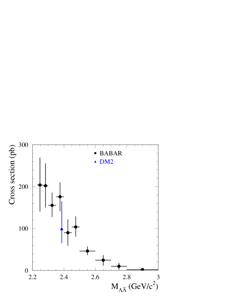
Figure 13: The $e^{+}e^{-}\to\mathchar 28931\relax\kern 1.99997pt\overline{\kern-1.99997pt\mathchar 28931\relax\kern 0.50003pt}\kern-0.50003pt{}$ cross section measured in the present experiment compared to the DM2DM2ll measurement.

Figure 14: The measured $\mathchar 28931\relax$ effective form factor.

The measured cross section for $e^{+}e^{-}\to\mathchar 28931\relax\kern 1.99997pt\overline{\kern-1.99997pt\mathchar 28931\relax\kern 0.50003pt}\kern-0.50003pt{}$ is shown in Fig. 14 and listed in Table 4. The quoted errors are statistical and systematic. The latter includes the systematic uncertainty in detection efficiency, the uncertainty in total integrated luminosity (1%), and the uncertainty in the radiative correction (1%). The only previous measurement of the $e^{+}e^{-}\to\mathchar 28931\relax\kern 1.99997pt\overline{\kern-1.99997pt\mathchar 28931\relax\kern 0.50003pt}\kern-0.50003pt{}$ cross section, $100^{+65}_{-35}$ pb at 2.386 GeV DM2ll , is in agreement with our results.

The $e^{+}e^{-}\to\mathchar 28931\relax\kern 1.99997pt\overline{\kern-1.99997pt\mathchar 28931\relax\kern 0.50003pt}\kern-0.50003pt{}$ cross section is a function of two form factors. Due to the poorly determined $|G_{E}/G_{M}|$ ratio they cannot be extracted from the data simultaneously with reasonable accuracy. We introduce an effective form factor (Eq.(4)) which is a linear combination of $|G_{E}|^{2}$ and $|G_{M}|^{2}$. The calculated effective form factor is shown in Fig. 14 and listed in Table 4.

III.6 $J/\psi$ and $\psi(2S)$ decays into $\mathchar 28931\relax\kern 1.99997pt\overline{\kern-1.99997pt\mathchar 28931\relax\kern 0.50003pt}\kern-0.50003pt{}$

The differential cross section for ISR production of a narrow resonance (vector meson $V$), such as $J/\psi$, decaying into the final state $f$ can be calculated using ivanch

$$\frac{{\rm d}\sigma(s,\theta_{\gamma}^{\ast})}{{\rm d}\cos{\theta_{\gamma}^{\ast}}}=\frac{12\pi^{2}\Gamma(V\to e^{+}e^{-}){\cal B}(V\to f)}{m_{V}\,s}\,W(s,x_{0},\theta_{\gamma}^{\ast}),$$ (11)

where $m_{V}$ and $\Gamma(V\to e^{+}e^{-})$ are the mass and electronic width of the vector meson $V$, $x_{0}=1-{m_{V}^{2}}/{s}$, and ${\cal B}(V\to f)$ is the branching fraction of $V$ into the final state $f$. Therefore, the measurement of the number of $J/\psi\to\mathchar 28931\relax\kern 1.99997pt\overline{\kern-1.99997pt\mathchar 28931\relax\kern 0.50003pt}\kern-0.50003pt{}$ decays in $e^{+}e^{-}\to\mathchar 28931\relax\kern 1.99997pt\overline{\kern-1.99997pt\mathchar 28931\relax\kern 0.50003pt}\kern-0.50003pt{}\gamma$ determines the product of the electronic width and the branching fraction: $\Gamma(J/\psi\to e^{+}e^{-}){\cal B}(J/\psi\to\mathchar 28931\relax\kern 1.99997pt\overline{\kern-1.99997pt\mathchar 28931\relax\kern 0.50003pt}\kern-0.50003pt{})$.

Figure 15: The $\mathchar 28931\relax\kern 1.99997pt\overline{\kern-1.99997pt\mathchar 28931\relax\kern 0.50003pt}\kern-0.50003pt{}$ mass spectra in the mass regions near the $J/\psi$ (a) and the $\psi(2S)$ (b). The arrows indicate the boundaries between the signal regions and sidebands.

The $\mathchar 28931\relax\kern 1.99997pt\overline{\kern-1.99997pt\mathchar 28931\relax\kern 0.50003pt}\kern-0.50003pt{}$ mass spectra for selected events in the $J/\psi$ and $\psi(2S)$ mass regions are shown in Fig. 15. We determine the number of resonance events by counting the events in the signal region indicated in Fig. 15, and subtracting the number in the two sidebands. The following numbers of $J/\psi$ and $\psi(2S)$ events are obtained: $N_{J/\psi}=142\pm 12$ and $N_{\psi(2S)}=17\pm 4$. A possible background due to $\psi\to p\overline{p}\pi^{+}\pi^{-}$ decay is estimated using the two-dimensional distribution of the masses of $\mathchar 28931\relax$ and $\kern 1.99997pt\overline{\kern-1.99997pt\mathchar 28931\relax\kern 0.50003pt}\kern-0.50003pt{}$ candidates. It is found to be $0.5^{+3.4}_{-0.5}$ events for $J/\psi$ and negligible for $\psi(2S)$.

The detection efficiency is estimated from MC simulation. The event generator uses the experimental data for the angular distribution of the $\mathchar 28931\relax$ in $J/\psi\to\mathchar 28931\relax\kern 1.99997pt\overline{\kern-1.99997pt\mathchar 28931\relax\kern 0.50003pt}\kern-0.50003pt{}$ decay. This distribution is described by $1+\alpha\cos^{2}\theta$ with $\alpha=0.65\pm 0.010$ MARKll ; DM2psi ; BESll . For the $\psi(2S)$ the value $\alpha=0.69$ predicted in Carimalo is used. The error in the detection efficiency due to the uncertainty of $\alpha$ is negligible for the $J/\psi$ and is taken to be 5% for the $\psi(2S)$. The efficiencies corrected for data-MC simulation differences are 0.062$\pm$0.004 for the $J/\psi$ and 0.059$\pm$0.005 for the $\psi(2S)$.

The cross section for $e^{+}e^{-}\to\psi\gamma\to\mathchar 28931\relax\kern 1.99997pt\overline{\kern-1.99997pt\mathchar 28931\relax\kern 0.50003pt}\kern-0.50003pt{}\gamma$ for $20^{\circ}<\theta_{\gamma}^{\ast}<160^{\circ}$ is calculated as

$$\sigma(20^{\circ}<\theta_{\gamma}^{\ast}<160^{\circ})=\frac{N_{\psi}}{\varepsilon\,R\,L},$$ (12)

yielding $(9.8\pm 0.9\pm 0.6)$ fb and $(1.2\pm 0.3\pm 0.1)$ fb for the $J/\psi$ and the $\psi(2S)$, respectively. The radiative-correction factor $R=\sigma/\sigma_{Born}$ is $1.007\pm 0.010$ for the $J/\psi$ and $1.011\pm 0.010$ for the $\psi(2S)$, obtained from MC simulation at the generator level.

The total integrated luminosity for the data sample is $(230\pm 2)$ fb^-1. From the measured cross sections and Eq. (11), the following products are determined:

$$\Gamma(J/\psi\to e^{+}e^{-}){\cal B}(J/\psi\to\mathchar 28931\relax\kern 1.99997pt\overline{\kern-1.99997pt\mathchar 28931\relax\kern 0.50003pt}\kern-0.50003pt{})=(10.7\pm 0.9\pm 0.7)\mbox{ eV},$$

$$\Gamma(\psi(2S)\to e^{+}e^{-}){\cal B}(\psi(2S)\to\mathchar 28931\relax\kern 1.99997pt\overline{\kern-1.99997pt\mathchar 28931\relax\kern 0.50003pt}\kern-0.50003pt{})=(1.5\pm 0.4\pm 0.1)\mbox{ eV}.$$

The systematic errors include the uncertainties in detection efficiency, integrated luminosity, and the radiative correction.

Using the world-average values of the electronic widths pdg , the $\psi\to\mathchar 28931\relax\kern 1.99997pt\overline{\kern-1.99997pt\mathchar 28931\relax\kern 0.50003pt}\kern-0.50003pt{}$ branching fractions are calculated to be

$${\cal B}(J/\psi\to\mathchar 28931\relax\kern 1.99997pt\overline{\kern-1.99997pt\mathchar 28931\relax\kern 0.50003pt}\kern-0.50003pt{})=(1.92\pm 0.21)\times 10^{-3},$$

$${\cal B}(\psi(2S)\to\mathchar 28931\relax\kern 1.99997pt\overline{\kern-1.99997pt\mathchar 28931\relax\kern 0.50003pt}\kern-0.50003pt{})=(6.0\pm 1.5)\times 10^{-4}.$$

Both results are higher than the current world-average values pdg : $(1.54\pm 0.19)\times 10^{-3}$ and $(2.5\pm 0.7)\times 10^{-4}$, but in reasonable agreement with the more precise recent measurements: $(2.03\pm 0.15)\times 10^{-3}$ by BES BESll and $(3.33\pm 0.25)\times 10^{-4}$ by CLEO cleo2s and BES bes2s .

Figure 16: The distribution of $\zeta_{fmax}$ for selected simulated events for $e^{+}e^{-}\to\mathchar 28931\relax\kern 1.99997pt\overline{\kern-1.99997pt\mathchar 28931\relax\kern 0.50003pt}\kern-0.50003pt{}\gamma$ with $M_{\mathchar 28931\relax\kern 1.39998pt\overline{\kern-1.39998pt\mathchar 28931\relax\kern 0.35002pt}\kern-0.35002pt{}}<2.8$ GeV/$c^{2}$.

Figure 17: The distribution of $\cos{\theta_{p\zeta}}$ for selected $e^{+}e^{-}\to\mathchar 28931\relax\kern 1.99997pt\overline{\kern-1.99997pt\mathchar 28931\relax\kern 0.50003pt}\kern-0.50003pt{}\gamma$ events with $M_{\mathchar 28931\relax\kern 1.39998pt\overline{\kern-1.39998pt\mathchar 28931\relax\kern 0.35002pt}\kern-0.35002pt{}}<2.8$ GeV/$c^{2}$ in simulation (a) and in data (b).

III.7 Measurement of the $\mathchar 28931\relax$ polarization

A nonzero relative phase $\phi$ between the electric and magnetic form factors leads to polarization of the outgoing baryons. The exact formula for the $\mathchar 28931\relax$ ($\kern 1.99997pt\overline{\kern-1.99997pt\mathchar 28931\relax\kern 0.50003pt}\kern-0.50003pt{}$) polarization vector $\zeta_{f}$ is given in the Appendix. The polarization is proportional to $\sin{\phi}$. The magnitude of the polarization $\zeta_{fmax}=\zeta_{f}(\phi=\pi/2)$ calculated under the assumption that $|G_{E}|=|G_{M}|$ for simulated $e^{+}e^{-}\to\mathchar 28931\relax\kern 1.99997pt\overline{\kern-1.99997pt\mathchar 28931\relax\kern 0.50003pt}\kern-0.50003pt{}\gamma$ events with $M_{\mathchar 28931\relax\kern 1.39998pt\overline{\kern-1.39998pt\mathchar 28931\relax\kern 0.35002pt}\kern-0.35002pt{}}<2.8$ GeV/$c^{2}$ is shown in Fig. 17. The simulated events were reweighted according to the $\mathchar 28931\relax\kern 1.99997pt\overline{\kern-1.99997pt\mathchar 28931\relax\kern 0.50003pt}\kern-0.50003pt{}$ mass spectrum observed in data. The average value of $\zeta_{fmax}$ is equal to 0.285. The $\mathchar 28931\relax$ polarization can be measured using the correlation between the direction of the $\mathchar 28931\relax$ polarization vector and the direction of the proton from $\mathchar 28931\relax$ decay:

$$\frac{{\rm d}N}{{\rm d}\cos{\theta_{p\zeta}}}=A(1+\alpha_{\mathchar 28931\relax}\zeta_{f}\cos{\theta_{p\zeta}}),$$ (13)

where $\theta_{p\zeta}$ is the angle between the polarization axis and the proton momentum in the $\mathchar 28931\relax$ rest frame, and $\alpha_{\mathchar 28931\relax}=0.642\pm 0.013$ pdg . For $\kern 1.99997pt\overline{\kern-1.99997pt\mathchar 28931\relax\kern 0.50003pt}\kern-0.50003pt{}$, $\alpha_{\kern 1.39998pt\overline{\kern-1.39998pt\mathchar 28931\relax\kern 0.35002pt}\kern-0.35002pt{}}=-\alpha_{\mathchar 28931\relax}$. The distribution of $\cos{\theta_{p\zeta}}$ for simulated $e^{+}e^{-}\to\mathchar 28931\relax\kern 1.99997pt\overline{\kern-1.99997pt\mathchar 28931\relax\kern 0.50003pt}\kern-0.50003pt{}\gamma$ events with $M_{\mathchar 28931\relax\kern 1.39998pt\overline{\kern-1.39998pt\mathchar 28931\relax\kern 0.35002pt}\kern-0.35002pt{}}<2.8$ GeV/$c^{2}$ (there is no $\mathchar 28931\relax$ polarization in the simulation) is shown in Fig. 17(a). We combine the $\mathchar 28931\relax$ and $\kern 1.99997pt\overline{\kern-1.99997pt\mathchar 28931\relax\kern 0.50003pt}\kern-0.50003pt{}$ distributions taking into account the different signs of $\alpha_{\mathchar 28931\relax}$ and $\alpha_{\kern 1.39998pt\overline{\kern-1.39998pt\mathchar 28931\relax\kern 0.35002pt}\kern-0.35002pt{}}$. Since the distribution is flat, we conclude that there is no dependence of the detection efficiency on $\cos{\theta_{p\zeta}}$. A fit to the distribution using a linear function gives slope consistent with zero.

The same distribution for data is shown in Fig. 17(b). In each angular interval the background is subtracted using the procedure described in Sec. III.2. The distribution is fitted using a linear function. The slope is found to be $0.020\pm 0.097$. The corresponding symmetric 90% CL interval for $\mathchar 28931\relax$ polarization averaged over the $\mathchar 28931\relax\kern 1.99997pt\overline{\kern-1.99997pt\mathchar 28931\relax\kern 0.50003pt}\kern-0.50003pt{}$ mass range from threshold to 2.8 GeV/$c^{2}$ is

$$-0.22<\zeta_{f}<0.28.$$

Under the assumption $|G_{E}|=|G_{M}|$ ($\bar{\zeta}_{fmax}=0.285$), which does not contradict the data, this interval can be converted to an interval for $\sin{\phi}$ as follows:

$$-0.76<\sin{\phi}<0.98.$$

Our statistics allow only very weak limits to be set on $\sin{\phi}$.

IV The reaction $e^{+}e^{-}\to\mathchar 28934\relax^{0}\kern 1.99997pt\overline{\kern-1.99997pt\mathchar 28934\relax}{}^{0}\gamma$

IV.1 Event selection

The $\mathchar 28934\relax^{0}$ hyperons are detected via the decay $\mathchar 28934\relax^{0}\to\mathchar 28931\relax\gamma$ (the branching fraction is 100% pdg ). Therefore, the preliminary selection of $e^{+}e^{-}\to\mathchar 28934\relax^{0}\kern 1.99997pt\overline{\kern-1.99997pt\mathchar 28934\relax}{}^{0}\gamma$ candidate events is similar to that for $e^{+}e^{-}\to\mathchar 28931\relax\kern 1.99997pt\overline{\kern-1.99997pt\mathchar 28931\relax\kern 0.50003pt}\kern-0.50003pt{}\gamma$. In addition, we require that an event contain at least two extra photons with energy greater than 30 MeV. To suppress combinatorial background from events not containing two $\mathchar 28931\relax$’s in the final state, we apply a tighter selection criterion on the mass of a $\mathchar 28931\relax$ ($\kern 1.99997pt\overline{\kern-1.99997pt\mathchar 28931\relax\kern 0.50003pt}\kern-0.50003pt{}$) candidate: $1.110<M_{p\pi^{-}}<1.122$ GeV/$c^{2}$.

For events passing the preliminary selection, we perform a kinematic fit to the $e^{+}e^{-}\to\mathchar 28931\relax\kern 1.99997pt\overline{\kern-1.99997pt\mathchar 28931\relax\kern 0.50003pt}\kern-0.50003pt{}\gamma\gamma\gamma$ hypothesis. The photon with highest $E^{\ast}_{\gamma}$ is assumed to be the ISR photon. The fitted momenta of two other photons and $\mathchar 28931\relax$-baryons are used to calculate $\mathchar 28931\relax\gamma$ and $\kern 1.99997pt\overline{\kern-1.99997pt\mathchar 28931\relax\kern 0.50003pt}\kern-0.50003pt{}\gamma$ invariant masses. For $\mathchar 28934\relax^{0}$ and $\kern 1.99997pt\overline{\kern-1.99997pt\mathchar 28934\relax}{}^{0}$ candidates these masses must to be in the range 1.155–1.23 GeV/$c^{2}$ (the nominal $\mathchar 28934\relax^{0}$ mass is 1.192642(24) GeV/$c^{2}$ pdg ). We require that an event contain at least one $\mathchar 28934\relax^{0}$ and one $\kern 1.99997pt\overline{\kern-1.99997pt\mathchar 28934\relax}{}^{0}$ candidate. For events with more than three photons we iterate over all possible photon combinations and find the one containing $\mathchar 28934\relax^{0}$ and $\kern 1.99997pt\overline{\kern-1.99997pt\mathchar 28934\relax}{}^{0}$ candidates and giving the lowest $\chi^{2}$ for the kinematic fit.

The distribution of the $\chi^{2}$ of the kinematic fit ($\chi^{2}_{\mathchar 28934\relax\mathchar 28934\relax}$) for simulated $e^{+}e^{-}\to\mathchar 28934\relax^{0}\kern 1.99997pt\overline{\kern-1.99997pt\mathchar 28934\relax}{}^{0}\gamma$ events is shown in Fig.20. We select data events with $\chi^{2}_{\mathchar 28934\relax\mathchar 28934\relax}<20$ for further analysis; as before, a $\chi^{2}$ control region ($20<\chi^{2}_{\mathchar 28934\relax\mathchar 28934\relax}<40$) is used for background estimation and subtraction.

Figure 18: The $\chi^{2}_{\mathchar 28934\relax\mathchar 28934\relax}$ distributions for simulated events for $e^{+}e^{-}\to\mathchar 28934\relax^{0}\kern 1.99997pt\overline{\kern-1.99997pt\mathchar 28934\relax}{}^{0}\gamma$.

Figure 19: The $\chi^{2}_{\mathchar 28931\relax\mathchar 28931\relax}$ distributions for simulated events for $e^{+}e^{-}\to\mathchar 28931\relax\kern 1.99997pt\overline{\kern-1.99997pt\mathchar 28931\relax\kern 0.50003pt}\kern-0.50003pt{}\gamma$ (solid histogram) and $e^{+}e^{-}\to\mathchar 28934\relax^{0}\kern 1.99997pt\overline{\kern-1.99997pt\mathchar 28934\relax}{}^{0}\gamma$ (dashed histogram).

Figure 20: The $\chi^{2}_{\mathchar 28931\relax\mathchar 28934\relax}$ distributions for simulated events for $e^{+}e^{-}\to\mathchar 28931\relax\kern 1.99997pt\overline{\kern-1.99997pt\mathchar 28934\relax}{}^{0}\gamma$ (solid histogram) and $e^{+}e^{-}\to\mathchar 28934\relax^{0}\kern 1.99997pt\overline{\kern-1.99997pt\mathchar 28934\relax}{}^{0}\gamma$ (dashed histogram).

To suppress background from $e^{+}e^{-}\to\mathchar 28931\relax\kern 1.99997pt\overline{\kern-1.99997pt\mathchar 28931\relax\kern 0.50003pt}\kern-0.50003pt{}\gamma$ and $e^{+}e^{-}\to\mathchar 28931\relax\kern 1.99997pt\overline{\kern-1.99997pt\mathchar 28934\relax}{}^{0}\gamma$ events with extra photons we also perform kinematic fits to the $\mathchar 28931\relax\kern 1.99997pt\overline{\kern-1.99997pt\mathchar 28931\relax\kern 0.50003pt}\kern-0.50003pt{}\gamma$ and $\mathchar 28931\relax\kern 1.99997pt\overline{\kern-1.99997pt\mathchar 28934\relax}{}^{0}\gamma$ hypotheses. The $\mathchar 28931\relax\kern 1.99997pt\overline{\kern-1.99997pt\mathchar 28934\relax}{}^{0}\gamma$ fit is a fit to the $e^{+}e^{-}\to\mathchar 28931\relax\kern 1.99997pt\overline{\kern-1.99997pt\mathchar 28931\relax\kern 0.50003pt}\kern-0.50003pt{}\gamma\gamma$ hypothesis. The photon with highest $E^{\ast}_{\gamma}$ is assumed to be the ISR photon. The other photon taken in combination with the $\mathchar 28931\relax$ or $\kern 1.99997pt\overline{\kern-1.99997pt\mathchar 28931\relax\kern 0.50003pt}\kern-0.50003pt{}$, must give an invariant mass value in the range 1.155–1.23 GeV/$c^{2}$, where the mass is calculated using fitted momenta. The $\chi^{2}_{\mathchar 28931\relax\mathchar 28931\relax}$ distributions for simulated events corresponding to $e^{+}e^{-}\to\mathchar 28931\relax\kern 1.99997pt\overline{\kern-1.99997pt\mathchar 28931\relax\kern 0.50003pt}\kern-0.50003pt{}\gamma$ and $e^{+}e^{-}\to\mathchar 28934\relax^{0}\kern 1.99997pt\overline{\kern-1.99997pt\mathchar 28934\relax}{}^{0}\gamma$ are shown in Fig.20. The requirement $\chi^{2}_{\mathchar 28931\relax\mathchar 28931\relax}>20$ rejects 93% of $\mathchar 28931\relax\kern 1.99997pt\overline{\kern-1.99997pt\mathchar 28931\relax\kern 0.50003pt}\kern-0.50003pt{}\gamma$ events and only 3% of signal events. Similarly, the $\chi^{2}_{\mathchar 28931\relax\mathchar 28934\relax}$ distributions for simulated events for $e^{+}e^{-}\to\mathchar 28931\relax\kern 1.99997pt\overline{\kern-1.99997pt\mathchar 28934\relax}{}^{0}\gamma$ and $e^{+}e^{-}\to\mathchar 28934\relax^{0}\kern 1.99997pt\overline{\kern-1.99997pt\mathchar 28934\relax}{}^{0}\gamma$ are shown in Fig.20. The requirement $\chi^{2}_{\mathchar 28931\relax\mathchar 28934\relax}>20$ again rejects 93% of $\mathchar 28931\relax\kern 1.99997pt\overline{\kern-1.99997pt\mathchar 28934\relax}{}^{0}\gamma$ events, but in this case removes 30% of the signal events. Data events with $\chi^{2}_{\mathchar 28931\relax\mathchar 28934\relax}<20$ are used to estimate the level of $\mathchar 28931\relax\kern 1.99997pt\overline{\kern-1.99997pt\mathchar 28934\relax}{}^{0}\gamma$ background.

The scatter plots of the invariant mass of the $\mathchar 28934\relax^{0}$ candidate versus the invariant mass of the $\kern 1.99997pt\overline{\kern-1.99997pt\mathchar 28934\relax}{}^{0}$ candidate for the selected data events and simulated $e^{+}e^{-}\to\mathchar 28934\relax^{0}\kern 1.99997pt\overline{\kern-1.99997pt\mathchar 28934\relax}{}^{0}\gamma$ events are shown in Figs. 21(a) and (b), respectively. Of the two possible $\mathchar 28931\relax\gamma$ and $\kern 1.99997pt\overline{\kern-1.99997pt\mathchar 28931\relax\kern 0.50003pt}\kern-0.50003pt{}\gamma$ combinations, we plot only the combination with the smaller value of $(M_{\mathchar 28931\relax\gamma}-m_{\mathchar 28934\relax})^{2}+(M_{\kern 1.39998pt\overline{\kern-1.39998pt\mathchar 28931\relax\kern 0.35002pt}\kern-0.35002pt{}\gamma}-m_{\mathchar 28934\relax})^{2}$, where $m_{\mathchar 28934\relax}$ is the nominal $\mathchar 28934\relax^{0}$ mass.

Figure 21: Scatter plots of the invariant mass of the $\mathchar 28934\relax^{0}$ candidate versus the invariant mass of the $\kern 1.99997pt\overline{\kern-1.99997pt\mathchar 28934\relax}{}^{0}$ candidate for selected data events (a), and simulated $e^{+}e^{-}\to\mathchar 28934\relax^{0}\kern 1.99997pt\overline{\kern-1.99997pt\mathchar 28934\relax}{}^{0}\gamma$ events (b).

The $\mathchar 28934\relax^{0}\kern 1.99997pt\overline{\kern-1.99997pt\mathchar 28934\relax}{}^{0}$ mass spectrum for the data events with the additional requirement that the $\mathchar 28934\relax^{0}$ and $\kern 1.99997pt\overline{\kern-1.99997pt\mathchar 28934\relax}{}^{0}$ candidate mass values satisfy $1.180<M_{\mathchar 28931\relax\gamma}<1.205$ GeV/$c^{2}$ (central box in Fig. 21(a)), is shown in Fig. 23.

Figure 22: The $\mathchar 28934\relax^{0}\kern 1.99997pt\overline{\kern-1.99997pt\mathchar 28934\relax}{}^{0}$ mass spectrum for the selected data events.

Figure 23: The $\mathchar 28931\relax\gamma$ and $\kern 1.99997pt\overline{\kern-1.99997pt\mathchar 28931\relax\kern 0.50003pt}\kern-0.50003pt{}\gamma$ invariant mass distribution for data (points with error bars) and simulated (histogram) events from the $J/\psi$ region.

An excess of signal events is seen at masses below 3.0 GeV/$c^{2}$. There are also about 20 events near the $J/\psi$ mass, corresponding to $J/\psi\to\mathchar 28934\relax^{0}\kern 1.99997pt\overline{\kern-1.99997pt\mathchar 28934\relax}{}^{0}$ decay. The two events near 3.7 GeV/$c^{2}$ may be due to $\psi(2S)\to\mathchar 28934\relax^{0}\kern 1.99997pt\overline{\kern-1.99997pt\mathchar 28934\relax}{}^{0}$ decay. The mass distribution for $\mathchar 28934\relax^{0}$ and $\kern 1.99997pt\overline{\kern-1.99997pt\mathchar 28934\relax}{}^{0}$candidates from the $J/\psi$ region is shown in Fig. 23. The spectrum is obtained as the difference of the spectrum from the region $3.05<M_{\mathchar 28934\relax\kern 1.39998pt\overline{\kern-1.39998pt\mathchar 28934\relax}{}}<3.15$ GeV/$c^{2}$ and that from the sideband region (3.00–3.05 and 3.15–3.20 GeV/$c^{2}$). We see that simulation reproduces the $\mathchar 28934\relax^{0}$ lineshape quite well.

IV.2 Background subtraction

Background processes can be divided into three classes, namely those with zero ($e^{+}e^{-}\to\mathchar 28931\relax\kern 1.99997pt\overline{\kern-1.99997pt\mathchar 28931\relax\kern 0.50003pt}\kern-0.50003pt{}\gamma$, $\mathchar 28931\relax\kern 1.99997pt\overline{\kern-1.99997pt\mathchar 28931\relax\kern 0.50003pt}\kern-0.50003pt{}\pi^{0}$, $\mathchar 28931\relax\kern 1.99997pt\overline{\kern-1.99997pt\mathchar 28931\relax\kern 0.50003pt}\kern-0.50003pt{}\pi^{0}\gamma$, … ), one ($e^{+}e^{-}\to\mathchar 28931\relax\kern 1.99997pt\overline{\kern-1.99997pt\mathchar 28934\relax}{}^{0}\gamma$, $\mathchar 28931\relax\kern 1.99997pt\overline{\kern-1.99997pt\mathchar 28934\relax}{}^{0}\pi^{0}$, $\mathchar 28931\relax\kern 1.99997pt\overline{\kern-1.99997pt\mathchar 28934\relax}{}^{0}\pi^{0}\gamma$, … ), and two $\mathchar 28934\relax^{0}$’s ($e^{+}e^{-}\to\mathchar 28934\relax^{0}\kern 1.99997pt\overline{\kern-1.99997pt\mathchar 28934\relax}{}^{0}\pi^{0}$, $\mathchar 28934\relax^{0}\kern 1.99997pt\overline{\kern-1.99997pt\mathchar 28934\relax}{}^{0}\pi^{0}\gamma$, … ) in the final state. To separate events with two $\mathchar 28934\relax^{0}$’s from events with no $\mathchar 28934\relax^{0}$’s and one $\mathchar 28934\relax^{0}$ we use the differences in their two-dimensional distributions of invariant mass values of the $\mathchar 28934\relax^{0}$ and $\kern 1.99997pt\overline{\kern-1.99997pt\mathchar 28934\relax}{}^{0}$ candidates.

Background events from $e^{+}e^{-}\to\mathchar 28934\relax^{0}\kern 1.99997pt\overline{\kern-1.99997pt\mathchar 28934\relax}{}^{0}\pi^{0}$ with an undetected low-energy photon or with merged photons from $\pi^{0}$ decay yield a low value of $\chi^{2}$ when reconstructed under the $\mathchar 28934\relax^{0}\kern 1.99997pt\overline{\kern-1.99997pt\mathchar 28934\relax}{}^{0}\gamma$ hypothesis, and can not be separated from the process under study. Special selection procedures are applied in order to estimate this background. The procedures are similar to those used to study background from $e^{+}e^{-}\to\mathchar 28931\relax\kern 1.99997pt\overline{\kern-1.99997pt\mathchar 28931\relax\kern 0.50003pt}\kern-0.50003pt{}\pi^{0}$ in Sec.III.2. No $\mathchar 28934\relax^{0}\kern 1.99997pt\overline{\kern-1.99997pt\mathchar 28934\relax}{}^{0}\pi^{0}$ candidates are found in data, and we estimate that the background from this process does not exceed 5 events. Assuming that the dibaryon mass spectrum in $e^{+}e^{-}\to\mathchar 28934\relax^{0}\kern 1.99997pt\overline{\kern-1.99997pt\mathchar 28934\relax}{}^{0}\pi^{0}$ is similar to that for $e^{+}e^{-}\to p\overline{p}\pi^{0}$ BADpp we find that about 70% of the $e^{+}e^{-}\to\mathchar 28934\relax^{0}\kern 1.99997pt\overline{\kern-1.99997pt\mathchar 28934\relax}{}^{0}\pi^{0}$ events are expected to have $\mathchar 28934\relax^{0}\kern 1.99997pt\overline{\kern-1.99997pt\mathchar 28934\relax}{}^{0}$ mass less than 3 GeV/$c^{2}$. Two-$\mathchar 28934\relax^{0}$ background other than that from $\mathchar 28934\relax^{0}\kern 1.99997pt\overline{\kern-1.99997pt\mathchar 28934\relax}{}^{0}\pi^{0}$ can be estimated using the difference in the $\chi^{2}$ distributions for signal and background events.

The $3\times 3$ two-dimensional histograms of $M_{\mathchar 28931\relax\gamma}$ vs $M_{\kern 1.39998pt\overline{\kern-1.39998pt\mathchar 28931\relax\kern 0.35002pt}\kern-0.35002pt{}\gamma}$ (dashed lines in Fig. 21) for events from three classes:

$$\chi^{2}_{\mathchar 28934\relax\mathchar 28934\relax}<20,\;\chi^{2}_{\mathchar 28931\relax\mathchar 28934\relax}>20,$$

$$20<\chi^{2}_{\mathchar 28934\relax\mathchar 28934\relax}<40,\;\chi^{2}_{\mathchar 28931\relax\mathchar 28934\relax}>20,$$

$$\chi^{2}_{\mathchar 28934\relax\mathchar 28934\relax}<20,\;\chi^{2}_{\mathchar 28931\relax\mathchar 28934\relax}<20,$$

are fitted simultaneously. The second histogram is used to determine two-$\mathchar 28934\relax^{0}$ background. From the third histogram we estimate the $e^{+}e^{-}\to\mathchar 28931\relax\kern 1.99997pt\overline{\kern-1.99997pt\mathchar 28934\relax}{}^{0}\gamma$ background. Each histogram is fitted using the following function:

$$N_{ij}=N_{2}f^{2\mathchar 28934\relax}_{i,j}+N_{1}f^{1\mathchar 28934\relax}_{i,j}+N_{0}f^{0\mathchar 28934\relax}_{i,j},$$

where $N_{0}$, $N_{1}$, and $N_{2}$ are the numbers of events with zero, one, and two $\mathchar 28934\relax^{0}$’s in the final state. The functions $f^{1\mathchar 28934\relax}$ and $f^{2\mathchar 28934\relax}$ are taken from $e^{+}e^{-}\to\mathchar 28931\relax\kern 1.99997pt\overline{\kern-1.99997pt\mathchar 28934\relax}{}^{0}\gamma$ and $e^{+}e^{-}\to\mathchar 28934\relax^{0}\kern 1.99997pt\overline{\kern-1.99997pt\mathchar 28934\relax}{}^{0}\gamma$ simulations. The probability density function for zero-$\mathchar 28934\relax^{0}$ events is the product of two identical linear functions of $M_{\mathchar 28931\relax\gamma}$ and $M_{\kern 1.39998pt\overline{\kern-1.39998pt\mathchar 28931\relax\kern 0.35002pt}\kern-0.35002pt{}\gamma}$ and a function taking into account the correlation between masses of the $\mathchar 28934\relax^{0}$ and $\kern 1.99997pt\overline{\kern-1.99997pt\mathchar 28934\relax}{}^{0}$ candidates. This last function is extracted from $e^{+}e^{-}\to\mathchar 28931\relax\kern 1.99997pt\overline{\kern-1.99997pt\mathchar 28931\relax\kern 0.50003pt}\kern-0.50003pt{}\gamma$ simulation. The correlation arises from our choice of one of the two possible combinations of $\mathchar 28931\relax$ and $\kern 1.99997pt\overline{\kern-1.99997pt\mathchar 28931\relax\kern 0.50003pt}\kern-0.50003pt{}$ candidates with photons, and is about 15% for the central mass bin.

In order to find the number of signal events and estimate the background we use the following relations:

$$N_{2}(\chi^{2}_{\mathchar 28934\relax\mathchar 28934\relax}<20,\;\chi^{2}_{\mathchar 28931\relax\mathchar 28934\relax}>20)=N_{2s}+N_{2b},$$

$$N_{2}(20<\chi^{2}_{\mathchar 28934\relax\mathchar 28934\relax}<40,\;\chi^{2}_{\mathchar 28931\relax\mathchar 28934\relax}>20)=\alpha_{1}N_{2s}+\beta_{1}N_{2b}.$$

$$N_{2}(\chi^{2}_{\mathchar 28934\relax\mathchar 28934\relax}<20,\;\chi^{2}_{\mathchar 28931\relax\mathchar 28934\relax}<20)=\alpha_{2}N_{2s}+\beta_{2}N_{2b},$$

$$N_{1}(\chi^{2}_{\mathchar 28934\relax\mathchar 28934\relax}<20,\;\chi^{2}_{\mathchar 28931\relax\mathchar 28934\relax}>20)=N_{1s}+N_{1b},$$

$$N_{1}(20<\chi^{2}_{\mathchar 28934\relax\mathchar 28934\relax}<40,\;\chi^{2}_{\mathchar 28931\relax\mathchar 28934\relax}>20)=\gamma_{1}N_{1s}+\delta_{1}N_{1b}.$$

$$N_{1}(\chi^{2}_{\mathchar 28934\relax\mathchar 28934\relax}<20,\;\chi^{2}_{\mathchar 28931\relax\mathchar 28934\relax}<20)=\gamma_{2}N_{1s}+\delta_{2}N_{1b},$$

where $N_{2s}$ is the number of signal $\mathchar 28934\relax^{0}\kern 1.99997pt\overline{\kern-1.99997pt\mathchar 28934\relax}{}^{0}\gamma$ events and $N_{2b}$ is the number of two-$\mathchar 28934\relax^{0}$ background events in the signal region ($\chi^{2}_{\mathchar 28934\relax\mathchar 28934\relax}<20,\;\chi^{2}_{\mathchar 28931\relax\mathchar 28934\relax}>20$), $N_{1s}$ is the number of $\mathchar 28931\relax\kern 1.99997pt\overline{\kern-1.99997pt\mathchar 28934\relax}{}^{0}\gamma$ events and $N_{1b}$ is the number of one-$\mathchar 28934\relax^{0}$ events from all other processes in the signal region; $N_{2s}$, $N_{2b}$, $N_{1s}$, and $N_{1b}$, are then free fit parameters. The coefficients $\alpha_{i}$, $\beta_{i}$, $\gamma_{i}$, and $\delta_{i}$ are obtained from simulation of $e^{+}e^{-}\to\mathchar 28934\relax^{0}\kern 1.99997pt\overline{\kern-1.99997pt\mathchar 28934\relax}{}^{0}\gamma$, $e^{+}e^{-}\to\mathchar 28934\relax^{0}\kern 1.99997pt\overline{\kern-1.99997pt\mathchar 28934\relax}{}^{0}\pi^{0}\gamma$, $e^{+}e^{-}\to\mathchar 28931\relax\kern 1.99997pt\overline{\kern-1.99997pt\mathchar 28934\relax}{}^{0}\gamma$, $e^{+}e^{-}\to\mathchar 28931\relax\kern 1.99997pt\overline{\kern-1.99997pt\mathchar 28934\relax}{}^{0}\pi^{0}\gamma$, respectively. For the coefficients most critical to the analysis, $\alpha_{1}=0.22\pm 0.03$ and $\beta_{1}=1.5\pm 0.3$, the errors include uncertainties due to the data-MC difference in the $\chi^{2}$ distributions for the kinematic fits. The other 6 free parameters are the numbers of zero-$\mathchar 28934\relax^{0}$ events in the three histograms, and the slopes of the linear functions describing the mass distributions for these events.

Table 5: Comparison of the fit results for $\mathchar 28934\relax^{0}\kern 1.99997pt\overline{\kern-1.99997pt\mathchar 28934\relax}{}^{0}$ masses below 3 GeV/$c^{2}$ and the predictions from JETSET simulation; $N_{2s}$, $N_{0}$, $N_{1}$, $N_{2b}$ are the fitted numbers of signal, zero-, one-, and two-$\mathchar 28934\relax^{0}$ background events in the signal region ($\chi^{2}_{\mathchar 28934\relax\mathchar 28934\relax}<20,\;\chi^{2}_{\mathchar 28931\relax\mathchar 28934\relax}>20$), respectively, $N_{\mathchar 28934\relax^{0}\kern 1.39998pt\overline{\kern-1.39998pt\mathchar 28934\relax}{}^{0}\pi^{0}}$ is expected number of background events from $e^{+}e^{-}\to\mathchar 28934\relax^{0}\kern 1.99997pt\overline{\kern-1.99997pt\mathchar 28934\relax}{}^{0}\pi^{0}$ process.

	$N_{2s}$	$N_{0}$	$N_{1}$	$N_{2b}$	$N_{\mathchar 28934\relax^{0}\kern 1.39998pt\overline{\kern-1.39998pt\mathchar 28934\relax}{}^{0}\pi^{0}}$
data	$18.1^{+7.8}_{-7.5}$	$11.3\pm 4.8$	$1.2\pm 0.6$	$2.8\pm 4.8$	$<4$
JETSET	$33\pm 5$	$3.1\pm 1.4$	$1.2\pm 0.8$	$<1.4$	$0.6\pm 0.6$

The fit results for $\mathchar 28934\relax^{0}\kern 1.99997pt\overline{\kern-1.99997pt\mathchar 28934\relax}{}^{0}$ masses below 3 GeV/$c^{2}$ are shown in Table 5, together with the predictions from JETSET simulation. The one-$\mathchar 28934\relax^{0}$ background is dominated by the $e^{+}e^{-}\to\mathchar 28931\relax\kern 1.99997pt\overline{\kern-1.99997pt\mathchar 28934\relax}{}^{0}\gamma$ process. The number of one-$\mathchar 28934\relax^{0}$ events from other processes is found to be consistent with zero. The numbers of $e^{+}e^{-}\to\mathchar 28934\relax^{0}\kern 1.99997pt\overline{\kern-1.99997pt\mathchar 28934\relax}{}^{0}\gamma$ and $e^{+}e^{-}\to\mathchar 28931\relax\kern 1.99997pt\overline{\kern-1.99997pt\mathchar 28934\relax}{}^{0}\gamma$ events with $\chi^{2}_{\mathchar 28931\relax\mathchar 28934\relax}<20$ are $7.7^{+3.4}_{-3.2}$ and $15.3^{+5.4}_{-7.7}$, respectively.

The fitting procedure was performed in five $\mathchar 28934\relax^{0}\kern 1.99997pt\overline{\kern-1.99997pt\mathchar 28934\relax}{}^{0}$ mass ranges, and the number of signal events found in each is listed in Table 7. For $\mathchar 28934\relax^{0}\kern 1.99997pt\overline{\kern-1.99997pt\mathchar 28934\relax}{}^{0}$ masses below 3 GeV/$c^{2}$ we observe an excess of signal events over background. The significance of the observation of $\mathchar 28934\relax^{0}\kern 1.99997pt\overline{\kern-1.99997pt\mathchar 28934\relax}{}^{0}$ production in the mass region below 3.0 GeV/$c^{2}$ is 2.9$\sigma$. For other mass bins we list upper limits at the 90% CL.

IV.3 Cross section and form factor

The cross section for $e^{+}e^{-}\to\mathchar 28934\relax^{0}\kern 1.99997pt\overline{\kern-1.99997pt\mathchar 28934\relax}{}^{0}$ is calculated from the $\mathchar 28934\relax^{0}\kern 1.99997pt\overline{\kern-1.99997pt\mathchar 28934\relax}{}^{0}$ mass spectrum according to Eqs.(9-10).

The detection efficiency is determined from MC simulation and then corrected for data-MC simulation differences in detector response. The model dependence of the detection efficiency due to the unknown $|G_{E}/G_{M}|$ ratio is estimated to be 5% (see Sec. III.4). The efficiency corrections summarized in Table 6 were discussed in Sec. III.4.

Table 6: The values of the various efficiency corrections for the process $e^{+}e^{-}\to\mathchar 28934\relax^{0}\kern 1.99997pt\overline{\kern-1.99997pt\mathchar 28934\relax}{}^{0}\gamma$.

effect	$\delta_{i}$, (%)
$\chi^{2}_{\mathchar 28934\relax\mathchar 28934\relax}<20$	$-2.0\pm 6.0$
track reconstruction	$-1.0\pm 3.8$
$\overline{p}$ nuclear interaction	$+1.0\pm 0.4$
PID	$+0.6\pm 0.6$
photon inefficiency	$-3.9\pm 0.9$
photon conversion	$+1.2\pm 0.6$
total	$-4.1\pm 7.2$

On the basis of our analysis of ISR processes with photons in the final state BAD5pi , we enlarge the systematic error in the correction for the $\chi^{2}$ selection interval. The correction for trigger inefficiency is removed, since for $e^{+}e^{-}\to\mathchar 28934\relax^{0}\kern 1.99997pt\overline{\kern-1.99997pt\mathchar 28934\relax}{}^{0}\gamma$, trigger inefficiency is less than 0.001 both in data and in MC simulation. The corrected detection efficiencies are listed in Table 7. The overall uncertainty in efficiency takes into account simulation statistical error, model uncertainty, the error in the $\mathchar 28931\relax\to p\pi^{-}$ branching fraction, and the uncertainty of the efficiency correction.

Table 7: The $\mathchar 28934\relax^{0}\kern 1.99997pt\overline{\kern-1.99997pt\mathchar 28934\relax}{}^{0}$ invariant mass interval ($M_{\mathchar 28934\relax\kern 1.39998pt\overline{\kern-1.39998pt\mathchar 28934\relax}{}}$), net number of signal events ($N_{s}$), detection efficiency ($\varepsilon$), ISR luminosity ($L$), measured cross section ($\sigma$), and effective form factor ($F$) for $e^{+}e^{-}\to\mathchar 28934\relax^{0}\kern 1.99997pt\overline{\kern-1.99997pt\mathchar 28934\relax}{}^{0}$. The quoted errors on $\sigma$ are statistical and systematic. For the form factor, the total error is listed.

$M_{\mathchar 28934\relax\kern 1.39998pt\overline{\kern-1.39998pt\mathchar 28934\relax}{}}$	$N_{s}$	$\varepsilon$	$L$	$\sigma$	$|F|$
(GeV/$c^{2}$)			(pb-1)	(pb)
2.385–2.600	$10.3_{-4.5}^{+4.4}$	$0.024\pm 0.002$	14.3	$30\pm 13\pm 3$	$0.090^{+0.018}_{-0.023}$
2.600–2.800	$6.5_{-3.8}^{+3.1}$	$0.025\pm 0.003$	14.7	$17^{+8}_{-10}\pm 2$	$0.047^{+0.010}_{-0.017}$
2.800–3.000	$1.4_{-3.2}^{+3.5}$	$0.026\pm 0.003$	16.1	$3.4^{+8.5}_{-7.8}\pm 0.4$	$0.021^{+0.018}_{-0.021}$
3.200–3.600	$<2.3$	$0.023\pm 0.003$	39.9	$<2.5$	$<0.019$
3.800–5.000	$<2.3$	$0.023\pm 0.002$	180.4	$<0.5$	$<0.011$

The measured values of the $e^{+}e^{-}\to\mathchar 28934\relax^{0}\kern 1.99997pt\overline{\kern-1.99997pt\mathchar 28934\relax}{}^{0}$ cross section are listed in Table 7, together with the effective form factor values calculated according to Eq.(4). The quoted errors on the cross section are statistical and systematic. The latter includes systematic uncertainty in detection efficiency, the uncertainty in total integrated luminosity (1%), and radiative correction uncertainty (1%). This is the first measurement of the $e^{+}e^{-}\to\mathchar 28934\relax^{0}\kern 1.99997pt\overline{\kern-1.99997pt\mathchar 28934\relax}{}^{0}$ cross section. The upper limit set by DM2 DM2ll at 2.386 GeV ( $<120$ pb) is consistent with our measurements.

Figure 24: The $\mathchar 28934\relax^{0}\kern 1.99997pt\overline{\kern-1.99997pt\mathchar 28934\relax}{}^{0}$ mass spectrum for the mass region near the $J/\psi$. The arrows indicate the boundaries between the signal region and sideband regions.

IV.4 $J/\psi$ decay into $\mathchar 28934\relax^{0}\kern 1.99997pt\overline{\kern-1.99997pt\mathchar 28934\relax}{}^{0}$

The $\mathchar 28934\relax^{0}\kern 1.99997pt\overline{\kern-1.99997pt\mathchar 28934\relax}{}^{0}$ mass spectrum for selected events in the $J/\psi$ mass region is shown in Fig. 24. We determine the number of resonance events by counting the events in the signal region indicated in Fig. 24 and subtracting the number in the two sidebands. The net number of $J/\psi$ decay events is then $30\pm 6$.

The detection efficiency is estimated from MC simulation. The event generator uses the experimental data on the $\mathchar 28934\relax^{0}$ angular distribution in $J/\psi\to\mathchar 28934\relax^{0}\kern 1.99997pt\overline{\kern-1.99997pt\mathchar 28934\relax}{}^{0}$ decay, which is $1+\alpha\cos^{2}theta$ with $\alpha=-0.1\pm 0.2$ MARKll ; DM2psi ; BESll . The error in the detection efficiency due to the uncertainty in $\alpha$ is negligible. The efficiency corrected for data-MC simulation differences is $\varepsilon$ = 0.022$\pm$0.002.

Using Eqs. (11,12) the following product is determined:

$$\Gamma(J/\psi\to e^{+}e^{-}){\cal B}(J/\psi\to\mathchar 28934\relax^{0}\kern 1.99997pt\overline{\kern-1.99997pt\mathchar 28934\relax}{}^{0})=(6.4\pm 1.2\pm 0.6)\mbox{ eV}.$$

The systematic error includes the uncertainties in detection efficiency, integrated luminosity, and in the radiative correction. Using the PDG value of the electronic width pdg , the $J/\psi\to\mathchar 28934\relax^{0}\kern 1.99997pt\overline{\kern-1.99997pt\mathchar 28934\relax}{}^{0}$ branching fraction is calculated to be

$${\cal B}(J/\psi\to\mathchar 28934\relax^{0}\kern 1.99997pt\overline{\kern-1.99997pt\mathchar 28934\relax}{}^{0})=(1.16\pm 0.26)\times 10^{-3}.$$

Our result is in agreement with the world average value $(1.31\pm 0.10)\times 10^{-3}$ pdg .

We also observe 2 events in the $\psi(2S)$ region with zero background, estimated from the sidebands. This number agrees with the $2.5\pm 0.4$ events expected from the measured branching fraction ${\cal B}(\psi(2S)\to\mathchar 28934\relax^{0}\kern 1.99997pt\overline{\kern-1.99997pt\mathchar 28934\relax}{}^{0})=(2.51\pm 0.31)\times 10^{-4}$ cleo2s ; bes2s .

V The reaction $e^{+}e^{-}\to\mathchar 28931\relax\kern 1.99997pt\overline{\kern-1.99997pt\mathchar 28934\relax}{}^{0}\gamma$

V.1 Event selection

The preliminary selection of $e^{+}e^{-}\to\mathchar 28931\relax\kern 1.99997pt\overline{\kern-1.99997pt\mathchar 28934\relax}{}^{0}\gamma$ events is similar to that for $e^{+}e^{-}\to\mathchar 28931\relax\kern 1.99997pt\overline{\kern-1.99997pt\mathchar 28931\relax\kern 0.50003pt}\kern-0.50003pt{}\gamma$. Additionally we require that an event candidate contain at least one extra photon with energy greater than 30 MeV. To suppress combinatorial background from events not containing two $\mathchar 28931\relax$’s in the final state we require that the mass of the $\mathchar 28931\relax$ ($\kern 1.99997pt\overline{\kern-1.99997pt\mathchar 28931\relax\kern 0.50003pt}\kern-0.50003pt{}$) satisfy $1.110<M_{p\pi^{-}}<1.122$ GeV/$c^{2}$.

For events passing the preliminary selection, we perform a kinematic fit to the $e^{+}e^{-}\to\mathchar 28931\relax\kern 1.99997pt\overline{\kern-1.99997pt\mathchar 28934\relax}{}^{0}\gamma$ hypothesis as described in Sec. IV.1. The $\chi^{2}_{\mathchar 28931\relax\mathchar 28934\relax}$ distribution for simulated $\mathchar 28931\relax\kern 1.99997pt\overline{\kern-1.99997pt\mathchar 28934\relax}{}^{0}\gamma$ events is shown in Fig. 25. We select the events with $\chi^{2}_{\mathchar 28931\relax\mathchar 28934\relax}<20$ for further analysis. The control region ($20<\chi^{2}_{\mathchar 28931\relax\mathchar 28934\relax}<40$) is used for background estimation and subtraction.

Figure 25: The $\chi^{2}_{\mathchar 28931\relax\mathchar 28934\relax}$ distributions for simulated $e^{+}e^{-}\to\mathchar 28931\relax\kern 1.99997pt\overline{\kern-1.99997pt\mathchar 28934\relax}{}^{0}\gamma$ events.

Figure 26: The $\chi^{2}_{\mathchar 28931\relax\mathchar 28931\relax}$ distributions for simulated $e^{+}e^{-}\to\mathchar 28931\relax\kern 1.99997pt\overline{\kern-1.99997pt\mathchar 28931\relax\kern 0.50003pt}\kern-0.50003pt{}\gamma$ events (solid histogram) and $e^{+}e^{-}\to\mathchar 28931\relax\kern 1.99997pt\overline{\kern-1.99997pt\mathchar 28934\relax}{}^{0}\gamma$ events(dashed histogram).

To suppress background resulting from $e^{+}e^{-}\to\mathchar 28931\relax\kern 1.99997pt\overline{\kern-1.99997pt\mathchar 28931\relax\kern 0.50003pt}\kern-0.50003pt{}\gamma$ events with an additional photon we perform a kinematic fit to the $\mathchar 28931\relax\kern 1.99997pt\overline{\kern-1.99997pt\mathchar 28931\relax\kern 0.50003pt}\kern-0.50003pt{}\gamma$ hypothesis and require that $\chi^{2}_{\mathchar 28931\relax\mathchar 28931\relax}>20$. The $\chi^{2}_{\mathchar 28931\relax\mathchar 28931\relax}$ distributions for simulated $e^{+}e^{-}\to\mathchar 28931\relax\kern 1.99997pt\overline{\kern-1.99997pt\mathchar 28931\relax\kern 0.50003pt}\kern-0.50003pt{}\gamma$ and $e^{+}e^{-}\to\mathchar 28931\relax\kern 1.99997pt\overline{\kern-1.99997pt\mathchar 28934\relax}{}^{0}\gamma$ events are shown in Fig. 26. The $\chi^{2}_{\mathchar 28931\relax\mathchar 28931\relax}>20$ cut rejects 95% of the $\mathchar 28931\relax\kern 1.99997pt\overline{\kern-1.99997pt\mathchar 28931\relax\kern 0.50003pt}\kern-0.50003pt{}\gamma$ events at the cost of 20% of the signal events.

The distribution of $\mathchar 28934\relax^{0}$ candidate invariant mass for data events passing the $\mathchar 28931\relax\kern 1.99997pt\overline{\kern-1.99997pt\mathchar 28934\relax}{}^{0}\gamma$ selection process is shown in Fig. 27. For each event we plot only the $\mathchar 28931\relax(\kern 1.99997pt\overline{\kern-1.99997pt\mathchar 28931\relax\kern 0.50003pt}\kern-0.50003pt{})\gamma$ combination closer to the nominal $\mathchar 28934\relax^{0}$ mass. The $\mathchar 28931\relax\kern 1.99997pt\overline{\kern-1.99997pt\mathchar 28934\relax}{}^{0}$ mass distribution for selected data events with invariant mass of the $\kern 1.99997pt\overline{\kern-1.99997pt\mathchar 28934\relax}{}^{0}$ candidate in the 1.185-1.205 GeV/$c^{2}$ range is shown in Fig. 28. We expect that the $e^{+}e^{-}\to\mathchar 28934\relax^{0}\kern 1.99997pt\overline{\kern-1.99997pt\mathchar 28934\relax}{}^{0}\gamma$ process results in a significant contribution to the selected event sample.

Figure 27: The distribution of the invariant mass of the $\mathchar 28934\relax^{0}$ and $\kern 1.99997pt\overline{\kern-1.99997pt\mathchar 28934\relax}{}^{0}$ candidates for the selected $\mathchar 28931\relax\kern 1.99997pt\overline{\kern-1.99997pt\mathchar 28934\relax}{}^{0}\gamma$ candidate.

Figure 28: The $\mathchar 28931\relax\kern 1.99997pt\overline{\kern-1.99997pt\mathchar 28934\relax}{}^{0}$ invariant mass spectrum for data events with the invariant mass of the $\mathchar 28934\relax^{0}$ candidate in the 1.185-1.205 GeV/$c^{2}$ range.

In particular, the peak in the $\mathchar 28931\relax\kern 1.99997pt\overline{\kern-1.99997pt\mathchar 28934\relax}{}^{0}$ mass spectrum near 3 GeV/$c^{2}$ is from $J/\psi\to\mathchar 28934\relax^{0}\kern 1.99997pt\overline{\kern-1.99997pt\mathchar 28934\relax}{}^{0}$ events with a missing or excluded photon.

V.2 Background subtraction

The background processes can be divided into three classes, namely those with zero ($e^{+}e^{-}\to\mathchar 28931\relax\kern 1.99997pt\overline{\kern-1.99997pt\mathchar 28931\relax\kern 0.50003pt}\kern-0.50003pt{}\gamma$, $\mathchar 28931\relax\kern 1.99997pt\overline{\kern-1.99997pt\mathchar 28931\relax\kern 0.50003pt}\kern-0.50003pt{}\pi^{0}$, $\mathchar 28931\relax\kern 1.99997pt\overline{\kern-1.99997pt\mathchar 28931\relax\kern 0.50003pt}\kern-0.50003pt{}\pi^{0}\gamma$, … ), one ($e^{+}e^{-}\to\mathchar 28931\relax\kern 1.99997pt\overline{\kern-1.99997pt\mathchar 28934\relax}{}^{0}\pi^{0}$, $\mathchar 28931\relax\kern 1.99997pt\overline{\kern-1.99997pt\mathchar 28934\relax}{}^{0}\pi^{0}\gamma$, … ), and two $\mathchar 28934\relax^{0}$’s ($e^{+}e^{-}\to\mathchar 28934\relax^{0}\kern 1.99997pt\overline{\kern-1.99997pt\mathchar 28934\relax}{}^{0}\gamma$, $\mathchar 28934\relax^{0}\kern 1.99997pt\overline{\kern-1.99997pt\mathchar 28934\relax}{}^{0}\pi^{0}$, $\mathchar 28934\relax^{0}\kern 1.99997pt\overline{\kern-1.99997pt\mathchar 28934\relax}{}^{0}\pi^{0}\gamma$, … ) in the final state. To separate one-$\mathchar 28934\relax^{0}$ events from events with no $\mathchar 28934\relax^{0}$ we use the difference in mass distribution for the respective $\mathchar 28934\relax^{0}$ ($\kern 1.99997pt\overline{\kern-1.99997pt\mathchar 28934\relax}{}^{0}$) candidates.

To determine two-$\mathchar 28934\relax^{0}$ background we select a clean sample of two-$\mathchar 28934\relax^{0}$ events. To do this the $\mathchar 28934\relax^{0}\kern 1.99997pt\overline{\kern-1.99997pt\mathchar 28934\relax}{}^{0}\gamma$ criteria (Sec. IV.1) are used with the additional requirements that $1.180<M_{\mathchar 28931\relax\gamma}<1.205$ GeV/$c^{2}$ for the $\mathchar 28934\relax^{0}$ and $\kern 1.99997pt\overline{\kern-1.99997pt\mathchar 28934\relax}{}^{0}$ candidates, and that $\chi^{2}_{\mathchar 28931\relax\mathchar 28934\relax}<100$. The latter requirement is needed to obtain a useful $M_{\mathchar 28931\relax\kern 1.39998pt\overline{\kern-1.39998pt\mathchar 28934\relax}{}}$ distribution. Using the ratio of detection efficiencies for two-$\mathchar 28934\relax^{0}$ and $\mathchar 28931\relax\kern 1.99997pt\overline{\kern-1.99997pt\mathchar 28934\relax}{}^{0}\gamma$ selections ($\kappa=0.80\pm 0.05$), we can convert the number of events in the two-$\mathchar 28934\relax^{0}$ sample to an estimate of the number of background events in the $\mathchar 28931\relax\kern 1.99997pt\overline{\kern-1.99997pt\mathchar 28934\relax}{}^{0}\gamma$ sample.

The background from $e^{+}e^{-}\to\mathchar 28931\relax\kern 1.99997pt\overline{\kern-1.99997pt\mathchar 28934\relax}{}^{0}\pi^{0}$ events with an undetected low-energy photon or with merged photons from $\pi^{0}$ decay cannot be separated from the process under study. The experimental data with special selection criteria are used to estimate this background. The procedure is similar to that used in the study of $e^{+}e^{-}\to\mathchar 28931\relax\kern 1.99997pt\overline{\kern-1.99997pt\mathchar 28931\relax\kern 0.50003pt}\kern-0.50003pt{}\pi^{0}$ background in Sec.III.2. We selected two $\mathchar 28934\relax^{0}\kern 1.99997pt\overline{\kern-1.99997pt\mathchar 28934\relax}{}^{0}\pi^{0}$ candidates with an expected background from $e^{+}e^{-}\to\mathchar 28931\relax\kern 1.99997pt\overline{\kern-1.99997pt\mathchar 28931\relax\kern 0.50003pt}\kern-0.50003pt{}\gamma$ and $e^{+}e^{-}\to\mathchar 28931\relax\kern 1.99997pt\overline{\kern-1.99997pt\mathchar 28934\relax}{}^{0}\gamma$ processes of $0.5\pm 0.2$ events. To suppress the $\mathchar 28931\relax\kern 1.99997pt\overline{\kern-1.99997pt\mathchar 28934\relax}{}^{0}\pi^{0}$ background in the $\mathchar 28931\relax\kern 1.99997pt\overline{\kern-1.99997pt\mathchar 28934\relax}{}^{0}\gamma$ sample we reject events with $0.10<M_{2\gamma}<0.17$ GeV/$c^{2}$, where $M_{2\gamma}$ is the invariant mass of the most energetic photon in an event and another photon with energy greater than 0.1 GeV. This removes about 1/3 of $\mathchar 28931\relax\kern 1.99997pt\overline{\kern-1.99997pt\mathchar 28934\relax}{}^{0}\pi^{0}$ events and less than 1% of signal events. After applying this selection criterion the rates at which $e^{+}e^{-}\to\mathchar 28931\relax\kern 1.99997pt\overline{\kern-1.99997pt\mathchar 28934\relax}{}^{0}\pi^{0}$ events are selected as $\mathchar 28931\relax\kern 1.99997pt\overline{\kern-1.99997pt\mathchar 28934\relax}{}^{0}\gamma$ or $\mathchar 28931\relax\kern 1.99997pt\overline{\kern-1.99997pt\mathchar 28934\relax}{}^{0}\pi^{0}$ are in the ratio $(2.1\pm 0.2)$, and the $\mathchar 28931\relax\kern 1.99997pt\overline{\kern-1.99997pt\mathchar 28934\relax}{}^{0}\pi^{0}$ background in the $\mathchar 28931\relax\kern 1.99997pt\overline{\kern-1.99997pt\mathchar 28934\relax}{}^{0}\gamma$ event sample is estimated to be $(3.1\pm 2.2)$ events. We assume that the dibaryon mass distribution for the $e^{+}e^{-}\to\mathchar 28931\relax\kern 1.99997pt\overline{\kern-1.99997pt\mathchar 28934\relax}{}^{0}\pi^{0}$ process is similar to that for the $e^{+}e^{-}\to p\overline{p}\pi^{0}$ process BADpp . In particular, about 70% of the $e^{+}e^{-}\to\mathchar 28931\relax\kern 1.99997pt\overline{\kern-1.99997pt\mathchar 28934\relax}{}^{0}\pi^{0}$ events have $\mathchar 28931\relax\kern 1.99997pt\overline{\kern-1.99997pt\mathchar 28934\relax}{}^{0}$ mass less than 2.9 GeV/$c^{2}$. Both observed $\mathchar 28931\relax\kern 1.99997pt\overline{\kern-1.99997pt\mathchar 28934\relax}{}^{0}\pi^{0}$ events lie in this mass region.

The one-$\mathchar 28934\relax^{0}$ background other than $\mathchar 28931\relax\kern 1.99997pt\overline{\kern-1.99997pt\mathchar 28934\relax}{}^{0}\pi^{0}$ is estimated using the difference in the $\chi^{2}$ distributions for signal and background events. Two histograms of $M_{\mathchar 28931\relax}\gamma$ for events with $\chi^{2}_{\mathchar 28931\relax\mathchar 28934\relax}<20$ and with $20<\chi^{2}_{\mathchar 28931\relax\mathchar 28934\relax}<40$ are fitted simultaneously to the sum of the distributions for signal and background

$$n_{i}=N_{1}H_{1i}+N_{2}H_{2i}+N_{0}H_{0i},$$ (14)

where $N_{1}$, $N_{2}$, and $N_{0}$ are the numbers of events containing one, two, and zero $\mathchar 28934\relax^{0}$’s in the final state, respectively. The one-$\mathchar 28934\relax^{0}$ events are the signal events with a possible contribution from the background processes $\mathchar 28931\relax\kern 1.99997pt\overline{\kern-1.99997pt\mathchar 28934\relax}{}^{0}\pi^{0}$, $\mathchar 28931\relax\kern 1.99997pt\overline{\kern-1.99997pt\mathchar 28934\relax}{}^{0}\pi^{0}\gamma$, etc. The function $H_{1}$ describing the mass distribution of one-$\mathchar 28934\relax^{0}$ events is calculated using $e^{+}e^{-}\to\mathchar 28931\relax\kern 1.99997pt\overline{\kern-1.99997pt\mathchar 28934\relax}{}^{0}\gamma$ simulation. The distribution of two-$\mathchar 28934\relax^{0}$ events is taken from $e^{+}e^{-}\to\mathchar 28934\relax^{0}\kern 1.99997pt\overline{\kern-1.99997pt\mathchar 28934\relax}{}^{0}\gamma$ simulation. The parameter $N_{2}$ is fixed by addition of the term $-\ln{f_{P}(n_{0};\mu_{0})}$ to minimize the likelihood function. Here $f_{P}$ is a Poisson distribution, $n_{0}$ is number of events in the two-$\mathchar 28934\relax^{0}$ sample described above and $\mu_{0}=\kappa rN_{2}$. The scale factor $\kappa=0.80\pm 0.05$ is found from $e^{+}e^{-}\to\mathchar 28934\relax^{0}\kern 1.99997pt\overline{\kern-1.99997pt\mathchar 28934\relax}{}^{0}\gamma$ simulation as the ratio of detection efficiencies for two-$\mathchar 28934\relax^{0}$ and $\mathchar 28931\relax\kern 1.99997pt\overline{\kern-1.99997pt\mathchar 28934\relax}{}^{0}\gamma$ selections. The factor $r\approx 1.1$ takes into account the purity of the two-$\mathchar 28934\relax^{0}$ sample, which is $(90\pm 5)\%$. It should be noted that the two-$\mathchar 28934\relax^{0}$ sample contains not only $\mathchar 28934\relax^{0}\kern 1.99997pt\overline{\kern-1.99997pt\mathchar 28934\relax}{}^{0}\gamma$ but also events from the processes $e^{+}e^{-}\to\mathchar 28934\relax^{0}\kern 1.99997pt\overline{\kern-1.99997pt\mathchar 28934\relax}{}^{0}\pi^{0}$, $\mathchar 28934\relax^{0}\kern 1.99997pt\overline{\kern-1.99997pt\mathchar 28934\relax}{}^{0}\pi^{0}\gamma$, etc. A similar approach is used to introduce the $\mathchar 28931\relax\kern 1.99997pt\overline{\kern-1.99997pt\mathchar 28934\relax}{}^{0}\pi^{0}$ background into the fit. The shape of the zero-$\mathchar 28934\relax^{0}$ background ($H_{0}$) is modeled using the mass distribution for the $e^{+}e^{-}\to\mathchar 28931\relax\kern 1.99997pt\overline{\kern-1.99997pt\mathchar 28931\relax\kern 0.50003pt}\kern-0.50003pt{}\gamma$ process. The distribution is parametrized as $H_{0}=(1+a_{0}(M_{\mathchar 28931\relax\gamma}-m_{\mathchar 28934\relax}))f(M_{\mathchar 28934\relax})$, where $m_{\mathchar 28934\relax}$ is nominal $\mathchar 28934\relax^{0}$ mass. The function $f(M_{\mathchar 28931\relax\gamma})$ describes the deviation from a linear function due to our choice of one of the two $\mathchar 28931\relax(\kern 1.99997pt\overline{\kern-1.99997pt\mathchar 28931\relax\kern 0.50003pt}\kern-0.50003pt{})\gamma$ combinations. This function is equal to unity at the end points of the mass interval, and is about 2 at the center. We checked that the function $H_{0}$ with $a_{0}$ as free parameter provides a good description of the mass distributions for simulated $e^{+}e^{-}\to\mathchar 28931\relax\kern 1.99997pt\overline{\kern-1.99997pt\mathchar 28931\relax\kern 0.50003pt}\kern-0.50003pt{}\pi^{0}$ and $e^{+}e^{-}\to\mathchar 28931\relax\kern 1.99997pt\overline{\kern-1.99997pt\mathchar 28931\relax\kern 0.50003pt}\kern-0.50003pt{}\pi^{0}\gamma$ events, and data $\mathchar 28931\relax\kern 1.99997pt\overline{\kern-1.99997pt\mathchar 28931\relax\kern 0.50003pt}\kern-0.50003pt{}\gamma$ events selected by requiring $\chi^{2}_{\mathchar 28931\relax\mathchar 28931\relax}<20$ and $\chi^{2}_{\mathchar 28931\relax\mathchar 28934\relax}<20$.

The one-$\mathchar 28934\relax^{0}$ background other than that from $\mathchar 28931\relax\kern 1.99997pt\overline{\kern-1.99997pt\mathchar 28934\relax}{}^{0}\pi^{0}$ is estimated from the fit according to Eq.(6). The coefficients $\beta_{sig}$ and $\beta_{bkg}$ are obtained from the signal and $\mathchar 28931\relax\kern 1.99997pt\overline{\kern-1.99997pt\mathchar 28934\relax}{}^{0}\pi^{0}\gamma$ simulation and take the values $0.15\pm 0.02$ and $1.5\pm 0.3$, respectively. Their errors are enlarged to take into account the data-MC simulation difference in the $\chi^{2}$ distributions resulting from the kinematic fits.

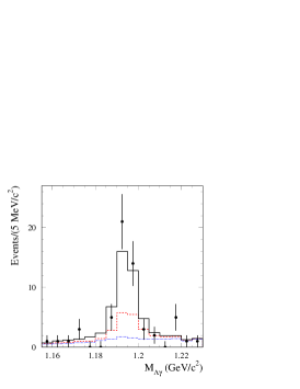
Figure 29: The distribution of the invariant mass of the $\mathchar 28934\relax^{0}$ ($\kern 1.99997pt\overline{\kern-1.99997pt\mathchar 28934\relax}{}^{0}$) candidate for data events with $M_{\mathchar 28931\relax\kern 1.39998pt\overline{\kern-1.39998pt\mathchar 28934\relax}{}}<2.9$ GeV/$c^{2}$ (points with error bars). The solid histogram shows the result of the fit described in the text. The dotted histogram shows the contribution of zero-$\mathchar 28934\relax^{0}$ background. The difference between dashed and dotted histograms is the contribution of two-$\mathchar 28934\relax^{0}$ background.

Figure 30: The distribution of selected data events (points with error bars) over chosen mass intervals. The histogram shows fitted background.

The fit results for $\mathchar 28931\relax\kern 1.99997pt\overline{\kern-1.99997pt\mathchar 28934\relax}{}^{0}$ masses below 2.9 GeV/$c^{2}$ are shown in Fig. 29 and summarized in Table 8, together with the predictions from the JETSET simulation.

Table 8: Comparison of the fit results for $\mathchar 28931\relax\kern 1.99997pt\overline{\kern-1.99997pt\mathchar 28934\relax}{}^{0}$ masses below 2.9 GeV/$c^{2}$ and the predictions from JETSET simulation; $N_{1s}$, $N_{0}$, $N_{1b}$, $N_{2}$ and $N_{\mathchar 28931\relax\kern 1.39998pt\overline{\kern-1.39998pt\mathchar 28934\relax}{}^{0}\pi^{0}}$ are the fitted numbers of signal, zero-, one-, two-$\mathchar 28934\relax^{0}$, and $\mathchar 28934\relax^{0}\kern 1.99997pt\overline{\kern-1.99997pt\mathchar 28934\relax}{}^{0}\pi^{0}$ background events with $\chi^{2}_{\mathchar 28931\relax\mathchar 28934\relax}<20$, respectively.

	$N_{1s}$	$N_{2}$	$N_{0}$	$N_{1b}$	$N_{\mathchar 28931\relax\kern 1.39998pt\overline{\kern-1.39998pt\mathchar 28934\relax}{}^{0}\pi^{0}}$
data	$24.1\pm 8.4$	$13.8\pm 4.4$	$17.0\pm 7.8$	$<5$	$3.1\pm 2.2$
JETSET	$50\pm 6$	$17\pm 3$	$3.0\pm 1.5$	$0.6\pm 0.6$	$1.2\pm 0.9$

The fitting procedure was performed in eight $\mathchar 28931\relax\kern 1.99997pt\overline{\kern-1.99997pt\mathchar 28934\relax}{}^{0}$ mass intervals, and the resulting data distribution is compared to the fitted background in Fig. 30. An excess of signal events over background is seen only for $\mathchar 28931\relax\kern 1.99997pt\overline{\kern-1.99997pt\mathchar 28934\relax}{}^{0}$ masses below 2.9 GeV/$c^{2}$. The number of signal events in each mass interval is listed in Table 10; 90% CL upper limits are given for the intervals with $M_{\mathchar 28931\relax\kern 1.39998pt\overline{\kern-1.39998pt\mathchar 28934\relax}{}}>2.9$ GeV/$c^{2}$. The significance of the observation of $\mathchar 28931\relax\kern 1.99997pt\overline{\kern-1.99997pt\mathchar 28934\relax}{}^{0}$ production in the mass region below 2.9 GeV/$c^{2}$ is 3.3$\sigma$.

V.3 Cross section and form factor

The cross section for $e^{+}e^{-}\to\mathchar 28931\relax\kern 1.99997pt\overline{\kern-1.99997pt\mathchar 28934\relax}{}^{0}$ is calculated from the $\mathchar 28931\relax\kern 1.99997pt\overline{\kern-1.99997pt\mathchar 28934\relax}{}^{0}$ mass spectrum according to Eqs.(9-10).

The detection efficiency is determined from MC simulation and then corrected for data-MC simulation differences in detector response. The model dependence of the detection efficiency due to the unknown $|G_{E}/G_{M}|$ ratio is estimated to be 5%. The efficiency corrections summarized in Table 9 were discussed in Secs. III.4 and IV.3.

Table 9: The values of the various efficiency corrections for the process $e^{+}e^{-}\to\mathchar 28931\relax\kern 1.99997pt\overline{\kern-1.99997pt\mathchar 28934\relax}{}^{0}\gamma$.

effect	$\delta_{i}$, (%)
$\chi^{2}_{\mathchar 28931\relax\mathchar 28934\relax}<20$	$-2.0\pm 6.0$
track reconstruction	$-1.0\pm 3.8$
$\overline{p}$ nuclear interaction	$+1.0\pm 0.4$
PID	$+0.6\pm 0.6$
photon inefficiency	$-2.6\pm 0.6$
photon conversion	$+0.8\pm 0.4$
total	$-3.2\pm 7.2$

Table 10: The $\mathchar 28931\relax\kern 1.99997pt\overline{\kern-1.99997pt\mathchar 28934\relax}{}^{0}$ invariant mass interval ($M_{\mathchar 28931\relax\kern 1.39998pt\overline{\kern-1.39998pt\mathchar 28934\relax}{}}$), net number of signal events ($N_{s}$), detection efficiency ($\varepsilon$), ISR luminosity ($L$), measured cross section ($\sigma$), and effective form factor ($F$) for $e^{+}e^{-}\to\mathchar 28934\relax^{0}\kern 1.99997pt\overline{\kern-1.99997pt\mathchar 28934\relax}{}^{0}$. The quoted errors on $\sigma$ are statistical and systematic. For the form factor, the total error is listed.

$M_{\mathchar 28931\relax\kern 1.39998pt\overline{\kern-1.39998pt\mathchar 28934\relax}{}}$	$N_{s}$	$\varepsilon$	$L$	$\sigma$	$|F|$
(GeV/$c^{2}$)			(pb-1)	(pb)
2.308–2.400	$9.4_{-4.1}^{+4.6}$	$0.035\pm 0.004$	5.70	$47^{+23}_{-21}\pm 5$	$0.102^{+0.023}_{-0.027}$
2.400–2.500	$8.7_{-4.7}^{+5.1}$	$0.041\pm 0.004$	6.52	$32^{+19}_{-18}\pm 4$	$0.068^{+0.018}_{-0.022}$
2.500–2.700	$4.2_{-4.4}^{+4.8}$	$0.042\pm 0.004$	14.02	$7.1^{+8.2}_{-7.5}\pm 0.7$	$0.029^{+0.014}_{-0.029}$
2.700–2.900	$1.8_{-2.3}^{+2.7}$	$0.041\pm 0.004$	15.38	$2.9^{+4.3}_{-3.7}\pm 0.3$	$0.018^{+0.011}_{-0.018}$
2.900–3.300	$<9.0$	$0.040\pm 0.004$	25.78	$<8.7$	$<0.033$
3.300–3.500	$<5.3$	$0.041\pm 0.005$	29.28	$<4.5$	$<0.025$
3.500–3.800	$<5.1$	$0.038\pm 0.005$	33.13	$<4.1$	$<0.026$
3.800–5.000	$<3.5$	$0.034\pm 0.004$	180.38	$<0.6$	$<0.011$

The corrected detection efficiencies are listed in Table 10. The uncertainty in efficiency takes into account simulation statistical error, model uncertainty, the error on the $\mathchar 28931\relax\to p\pi^{-}$ branching fraction, and the uncertainty in the efficiency correction.

The measured values of the $e^{+}e^{-}\to\mathchar 28931\relax\kern 1.99997pt\overline{\kern-1.99997pt\mathchar 28934\relax}{}^{0}$ cross section are listed in Table 10, together with those of the effective form factor. The quoted cross section errors are statistical and systematic. The latter includes systematic uncertainty in detection efficiency, the error on the total integrated luminosity (1%), and the radiative correction uncertainty (1%). This is the first measurement of the $e^{+}e^{-}\to\mathchar 28931\relax\kern 1.99997pt\overline{\kern-1.99997pt\mathchar 28934\relax}{}^{0}$ cross section. The upper limit set by DM2 DM2ll at 2.386 GeV ( $<75$ pb) is consistent with our results.

Assuming that all events in the 2.90–3.30 GeV/$c^{2}$ mass range result from $J/\psi\to\mathchar 28931\relax\kern 1.99997pt\overline{\kern-1.99997pt\mathchar 28934\relax}{}^{0}$ decay we obtain an upper limit for the $J/\psi\to\mathchar 28931\relax\kern 1.99997pt\overline{\kern-1.99997pt\mathchar 28934\relax}{}^{0}$ branching fraction ${\cal B}(J/\psi\to\mathchar 28931\relax\kern 1.99997pt\overline{\kern-1.99997pt\mathchar 28934\relax}{}^{0})<2\times 10^{-4}$, which is slightly higher than the only other estimate, ${\cal B}(J/\psi\to\mathchar 28931\relax\kern 1.99997pt\overline{\kern-1.99997pt\mathchar 28934\relax}{}^{0})<1.5\times 10^{-4}$ mark1 .

VI Summary

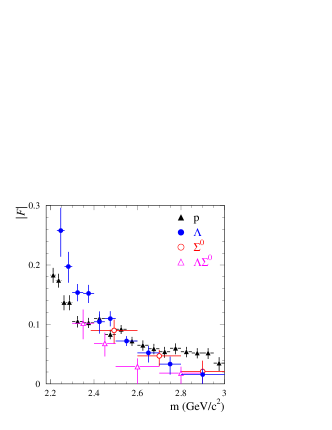
Figure 31: The measured dependence of the baryon form factors on dibaryon invariant mass. The proton data are taken from Ref. BADpp .

The processes $e^{+}e^{-}\to\mathchar 28931\relax\kern 1.99997pt\overline{\kern-1.99997pt\mathchar 28931\relax\kern 0.50003pt}\kern-0.50003pt{}\gamma$, $\mathchar 28931\relax\kern 1.99997pt\overline{\kern-1.99997pt\mathchar 28934\relax}{}^{0}\gamma$, and $\mathchar 28934\relax^{0}\kern 1.99997pt\overline{\kern-1.99997pt\mathchar 28934\relax}{}^{0}\gamma$ have been studied for dibaryon invariant mass up to 5 GeV/$c^{2}$. From the measured dibaryon mass spectra we obtained the $e^{+}e^{-}\to\mathchar 28931\relax\kern 1.99997pt\overline{\kern-1.99997pt\mathchar 28931\relax\kern 0.50003pt}\kern-0.50003pt{}$, $\mathchar 28931\relax\kern 1.99997pt\overline{\kern-1.99997pt\mathchar 28934\relax}{}^{0}$, and $\mathchar 28934\relax^{0}\kern 1.99997pt\overline{\kern-1.99997pt\mathchar 28934\relax}{}^{0}$ cross sections and baryon effective form factors. Our results on the measurements of the various baryon form factors for dibaryon invariant masses above $\mathchar 28931\relax\kern 1.99997pt\overline{\kern-1.99997pt\mathchar 28931\relax\kern 0.50003pt}\kern-0.50003pt{}$ threshold are shown in Fig. 31.

For $e^{+}e^{-}\to\mathchar 28931\relax\kern 1.99997pt\overline{\kern-1.99997pt\mathchar 28931\relax\kern 0.50003pt}\kern-0.50003pt{}\gamma$ we analyzed the $\mathchar 28931\relax$ angular distributions in the mass range from threshold to 2.8 GeV/$c^{2}$ and extracted the $|G_{E}/G_{M}|$ ratio. Our results are

$$|G_{E}/G_{M}|=1.73^{+0.99}_{-0.57}\;\;\mbox{ for 2.23--2.40 GeV}/c^{2},$$

$$|G_{E}/G_{M}|=0.71^{+0.66}_{-0.71}\;\;\mbox{ for 2.40--2.80 GeV}/c^{2},$$

and are consistent both with $|G_{E}/G_{M}|=1$ and with the results for $e^{+}e^{-}\to p\overline{p}$ BADpp , where this ratio was found to be significantly greater than unity near threshold.

The measurement of the $\mathchar 28931\relax$ polarization enables the extraction of the relative phase between the $\mathchar 28931\relax$ electric and magnetic form factors. The limited statistics of the present experiment allow us to set only very weak limits on this phase:

$$-0.76<\sin{\phi}<0.98.$$

From the events in the $J/\psi$ and $\psi(2S)$ regions the products,

$$\Gamma(J/\psi\to e^{+}e^{-}){\cal B}(J/\psi\to\mathchar 28931\relax\kern 1.99997pt\overline{\kern-1.99997pt\mathchar 28931\relax\kern 0.50003pt}\kern-0.50003pt{})=(10.7\pm 0.9\pm 0.7)\mbox{ eV},$$

$$\Gamma(J/\psi\to e^{+}e^{-}){\cal B}(J/\psi\to\mathchar 28934\relax^{0}\kern 1.99997pt\overline{\kern-1.99997pt\mathchar 28934\relax}{}^{0})=(6.4\pm 1.2\pm 0.6)\mbox{ eV},$$

$$\Gamma(\psi(2S)\to e^{+}e^{-}){\cal B}(\psi(2S)\to\mathchar 28931\relax\kern 1.99997pt\overline{\kern-1.99997pt\mathchar 28931\relax\kern 0.50003pt}\kern-0.50003pt{})=(1.5\pm 0.4\pm 0.1)\mbox{ eV},$$

have been measured, and, using the known $e^{+}e^{-}$ partial widths, the corresponding branching ratios have been obtained:

$${\cal B}(J/\psi\to\mathchar 28931\relax\kern 1.99997pt\overline{\kern-1.99997pt\mathchar 28931\relax\kern 0.50003pt}\kern-0.50003pt{})=(1.92\pm 0.21)\times 10^{-3},$$

$${\cal B}(J/\psi\to\mathchar 28934\relax^{0}\kern 1.99997pt\overline{\kern-1.99997pt\mathchar 28934\relax}{}^{0})=(1.16\pm 0.26)\times 10^{-3},$$

$${\cal B}(\psi(2S)\to\mathchar 28931\relax\kern 1.99997pt\overline{\kern-1.99997pt\mathchar 28931\relax\kern 0.50003pt}\kern-0.50003pt{})=(6.0\pm 1.5)\times 10^{-4}.$$

*

Appendix A Angular distributions and $\mathchar 28931\relax$ polarization in the $e^{+}e^{-}\to\mathchar 28931\relax\kern 1.99997pt\overline{\kern-1.99997pt\mathchar 28931\relax\kern 0.50003pt}\kern-0.50003pt{}\gamma$ reaction

The formulae given in this section are taken from Ref. dkm . The process $e^{+}e^{-}\to\mathchar 28931\relax\kern 1.99997pt\overline{\kern-1.99997pt\mathchar 28931\relax\kern 0.50003pt}\kern-0.50003pt{}\gamma$ is considered in the $e^{+}e^{-}$ center-of-mass frame, where the electron has momentum $p$ and energy $\varepsilon$, and the photon has momentum $k$ and energy $\omega$. The $\mathchar 28931\relax$ momentum $P$ is given in the $\mathchar 28931\relax\kern 1.99997pt\overline{\kern-1.99997pt\mathchar 28931\relax\kern 0.50003pt}\kern-0.50003pt{}$ rest frame. The differential cross section summed over the polarization of one of the final particles is given by

$${\rm d}\sigma=\frac{\alpha^{3}P{\rm d}^{3}k{\rm d}\Omega_{\mathchar 28931\relax}}{16\pi^{2}\omega\varepsilon^{2}Q^{3}[1-({\mathbf{n}}\cdot\mbox{\boldmath$\nu$})^{2}]}{\cal A}(1+\mbox{\boldmath$\zeta_{f}$}\cdot{\mathbf{s}}),\;\;{\cal A}=2|G_{M}|^{2}(1+N^{2})+\left(\frac{4m_{\mathchar 28931\relax}^{2}}{Q^{2}}|G_{E}|^{2}-|G_{M}|^{2}\right)([{\mathbf{n}}\times{\mathbf{f}}]^{2}+[{\mathbf{N}}\times{\mathbf{f}}]^{2}),$$

$$\mbox{\boldmath$\zeta_{f}$}=\frac{4m_{\mathchar 28931\relax}}{Q{\cal A}}\mbox{Im}(G_{E}^{\ast}G_{M})\left(({\mathbf{n}}\cdot{\mathbf{f}})[{\mathbf{n}}\times{\mathbf{f}}]+({\mathbf{N}}\cdot{\mathbf{f}})[{\mathbf{N}}\times{\mathbf{f}}]\right);\;\;\;\;{\mathbf{n}}=\frac{{\mathbf{k}}}{\omega},\;\mbox{\boldmath$\nu$}=\frac{{\mathbf{p}}}{\varepsilon},\;{\mathbf{N}}=\frac{\mbox{\boldmath$\nu$}+(\gamma-1)({\mathbf{n}}\cdot\mbox{\boldmath$\nu$}){\mathbf{n}}}{\sqrt{\gamma^{2}-1}},$$

$$N^{2}=({\mathbf{n}}\cdot\mbox{\boldmath$\nu$})^{2}+\frac{1}{\gamma^{2}-1},\;\gamma=\frac{2\varepsilon-\omega}{Q},\;Q=\sqrt{\varepsilon(\varepsilon-\omega)},\;P=|{\mathbf{P}}|=\sqrt{Q^{2}/4-m_{\mathchar 28931\relax}^{2}},\;{\mathbf{f}}=\frac{{\mathbf{P}}}{P}.$$

Here ${\mathbf{s}}$ and $\zeta_{f}$ are the spin and polarization vectors of the $\mathchar 28931\relax$ in its rest frame.

References

(1)
B. Aubert et al. [BABAR Collaboration],
Phys. Rev. D 73, 012005 (2006).
(2)
G. Bonneau and F. Martin, Nucl. Phys. B 27, 381 (1971).
(3)
L. V. Kardapoltzev, Bachelor’s thesis, Novosibirsk State University,
2007 (unpublished).
(4)
A. Z. Dubnickova, S. Dubnicka and M. P. Rekalo,
Nuovo Cim. A 109, 241 (1996).
(5)
H. Czyz, A. Grzelinska and J. H. Kuhn,
Phys. Rev. D 75, 074026 (2007).
(6)
D. Bisello et al. [DM2 Collaboration],
Z. Phys. C 48, 23 (1990).
(7) B. Aubert et al. [BABAR Collaboration],
Nucl. Instr. and Meth. A 479, 1 (2002).
(8)
G. Rodrigo et al., Eur. Phys. J. C 24, 71 (2002).
(9)
H. Czyz et al., Eur. Phys. J. C 35, 527 (2004).
(10) S. Agostinelli et al. [GEANT4 Collaboration],
Nucl. Instr. and Meth. A 506, 250 (2003).
(11)
T. Sjöstrand, Comput. Phys. Commun. 82, 74 (1994).
(12)
M. Caffo, H. Czyz, and E. Remiddi, Nuo. Cim. 110A, 515 (1997);
Phys. Lett. B 327, 369 (1994).
(13)
W.-M. Yao et al. [Particle Data Group],
J. Phys. G 33, 1 (2006).
(14)
M. W. Eaton et al. [MARKII Collaboration],
Phys. Rev. D 29, 804 (1984).
(15)
D. Pallin et al. [DM2 Collaboration],
Nucl. Phys. B 292, 653 (1987).
(16)
M. Ablikim et al. [BES Collaboration],
Phys. Lett. B 632, 181 (2006).
(17)
J. Haidenbauer, H. W. Hammer, U. G. Meissner and A. Sibirtsev,
Phys. Lett. B 643, 29 (2006).
(18)
V. F. Dmitriev and A. I. Milstein,
Nucl. Phys. Proc. Suppl. 162, 53 (2006).
(19)
B. Aubert et al. [BABAR Collaboration],
Phys. Rev. D 71, 052001 (2005).
(20)
M. Benayoun et al., Mod. Phys. Lett. A 14, 2605 (1999).
(21)
C. Carimalo,
Int. J. Mod. Phys. A 2, 249 (1987).
(22)
T. K. Pedlar et al. [CLEO Collaboration],
Phys. Rev. D 72, 051108 (2005).
(23)
M. Ablikim et al. [BES Collaboration],
Phys. Lett. B 648, 149 (2007).
(24)
B. Aubert et al. [BABAR Collaboration],
Phys. Rev. D 73, 052003 (2006).
(25)
A. I. Milstein, private communication.
(26)
I. Peruzzi et al. [MARKI Collaboration],
Phys. Rev. D 17, 2901 (1978).