Fluctuations in Nonequilibrium Statistical Mechanics: Models, Mathematical Theory, Physical Mechanisms

Abstract

The fluctuations in nonequilibrium systems are under intense theoretical and experimental investigation. Topical “fluctuation relations” describe symmetries of the statistical properties of certain observables, in a variety of models and phenomena. They have been derived in deterministic and, later, in stochastic frameworks. Other results first obtained for stochastic processes, and later considered in deterministic dynamics, describe the temporal evolution of fluctuations. The field has grown beyond expectation: research works and different perspectives are proposed at an ever faster pace. Indeed, understanding fluctuations is important for the emerging theory of nonequilibrium phenomena, as well as for applications, such as those of nanotechnological and biophysical interest. However, the links among the different approaches and the limitations of these approaches are not fully understood. We focus on these issues, providing: a) analysis of the theoretical models; b) discussion of the rigorous mathematical results; c) identification of the physical mechanisms underlying the validity of the theoretical predictions, for a wide range of phenomena.

1 Introduction

The study of fluctuations in statistical mechanics dates back to Einstein’s 1905 seminal work on the Brownian motion [1], in which the first fluctuation-dissipation relation was given, and to Einstein’s 1910 paper which turned Boltzmann’s entropy formula in one expression for the probability of a fluctuation out of an equilibrium state [2]. Of the many authors who continued Einstein’s work, we can recall but a few. In 1927, Ornstein derived the fluctuation-dissipation relation for the random force acting on a Brownian particle [3]. In 1928, Nyquist obtained a formula for the spectral densities and correlation functions of the thermal noise in linear electrical circuits, in terms of their impedance [4], which applies to mechanical systems as well. In 1931, Onsager obtained the complementary result to that of Nyquist: the calculation of the transport coefficients from the observation of the thermal fluctuations [5, 6]. The fluctuation-dissipation theorem and the theory of transport coefficients received great impulse in the 1950’s, thanks to the works of authors such as Callen, Welton, R. F. Greene, [7, 8], and M. S.  Green and Kubo [9, 10, 11, 12]. In 1953, Onsager and Machlup provided a natural generalization to fluctuation paths of Einstein’s formula for the probability of a fluctuation value [13, 14]. In 1967, Alder and Wainwright discovered long time tails in the velocity autocorrelation functions, which implied the non-existence of the self-diffusion coefficient, in two dimensions [15]. Anomalous divergent behaviour of the transport coefficients was studied also by Kadanoff and Swift, for systems near a critical point [16]. Closely connected with the long time tails is the phenomenon of long range correlations in nonequilibrium steady states, which was pointed out and studied by a number of authors, including Cohen, Dorfman, Kirkpatrick, Oppenheim, Procaccia, Ronis, Spohn [17, 18, 19]. Nonequilibrium fluctuation theorems have been obtained also by Hänggi and Thomas [20, 21]. The transient time correlation function formalism, which yields an exact relation between nonlinear steady state response and transient fluctuations in the thermodynamic fluxes, has been developed by Visscher, Dufty, Lindenfeld, Cohen, Evans and Morriss [22, 23, 24, 25]. Under some differentiability conditions, Boffetta et al.  and Falcioni et al. [26, 27] obtained a fluctuation response relation, which applies to states that can be very far from equilibrium. Independently, Ruelle proved that those conditions are met by axiom A systems, and obtained the same fluctuation response relation [28].

This necessarily brief and incomplete account shows that the object of research has gradually shifted from equilibrium to nonequilibrium problems. But while the equilibrium theory can be considered quite satisfactory and complete, the same cannot be said of the nonequilibrium theory, which concerns a much wider range of phenomena.

The 1993 paper by Evans, Cohen and Morriss [29], on the fluctuations of the entropy production rate of a deterministic particle system, modeling a shearing fluid, provided a unifying framework for a variety of nonequilibrium phenomena, under a mathematical expression nowadays called Fluctuation Relation (FR). Then, fluctuation relations for transient states were proved by Evans and Searles in 1994 [30, 31], while Gallavotti and Cohen obtained steady state relations for systems whose dynamics can be considered to be Anosov, in 1995 [32, 33]. The FR is one example of the few exact, general results on nonequilibrium systems, and extends the Green-Kubo and Onsager relations to far from equilibrium states [34, 35, 36].

The subject of the present review is the FR for deterministic particle systems, with an eye on open problems, and on the interplay of mathematical and physical investigations. The connection with FRs for stochastic processes is also discussed. Section 2 summarizes the history of FRs. Section 3 illustrates a class of deterministic, time reversal invariant models of nonequilibrium systems, relevant in the study of FRs, and reports some new results. Sections 4 and 5 illustrate, respectively, the mathematical theory, developed for the phase space contraction rate, and the physical mechanisms underlying the validity of FRs for quantities such as the energy dissipation rate. Section 6 is devoted to the Jarzynski and Crooks relations and to their connection with the FRs. Sections 7 and 8 illustrate, respectively, some stochastic versions of the FRs, including the Van Zon-Cohen relation, and the theory developed by Jona-Lasinio and collaborators. Section 9 describes some numerical and experimental tests of the FRs. Concluding remarks are made in Section 10.

1.1 Prologue

Why focus on deterministic rather than stochastic FRs? The stochastic approach seems to produce easily the same results that the dynamical approach obtains with much effort. Kurchan says that this is the case because the stochastic description, commonly assumed to be a reduced (mesoscopic) representation of the “chaotic” microscopic dynamics, is free from the intricate fractal structures of deterministic dynamics [37]. Then, considering that the mathematical approach to deterministic FRs makes assumptions which, in general, cannot be directly verified [37], one may conclude that the stochastic approach is to be preferred to the deterministic one. In reality, there are various reasons to consider deterministic systems. For instance, fundamental issues, like irreversibility, can hardly be understood within the framework of the intrinsically irreversible stochastic processes [37]. Also, stochastic descriptions assume that averages characterize single systems. This is justified only if the microscopic dynamics are sufficiently “chaotic” that the average behaviour is established within mesoscopic time scales [38], as happens in Thermodynamics, thanks to the interactions among the particles, and to their very large number. However, in certain circumstances particles do not interact or interact more with their environment than with each other [39, 40]; the number of particles may be small; strong external drivings may produce ordered phases; etc. In such cases, the local thermodynamic equilibrium is violated and average behaviours do not characterize single systems, they only characterize ensembles. Furthermore, the identification of physical observables in stochastic processes is often affected by ambiguities. As far as the microscopic-mesoscopic connection is concerned only a few models, like the Lorentz gas [41, 42, 43], have been mapped into Markov processes [44], and the mapping concerns the phase space, not the real space.

Adding that certain results obtained for stochastic processes were not obvious in terms of reversible equations of motion (cf.  Section 8 on temporal asymmetries), while results such as the FRs were not obvious in the stochastic description, we conclude that the deterministic and the stochastic approaches are both necessary to provide a unifying framework, for the field of nonequilibrium physics, and its applications. In this review, we mainly focus on deterministic FRs, but we also discuss their relations with the stochastic ones.

We illustrate two classes of FRs, transient and steady state FRs. The transient FRs concern the time dependent response to external drivings of ensembles of systems, or ensembles of experiments, and hold under very general conditions (time reversibility suffices for those obtained by Evans and Searles; Hamiltonian dynamics suffices for the one derived by Jarzynski). These relations have interesting applications in the study of nanotechnological devices and of biological systems [45], and hold for arbitrarily short times. The steady state FRs have similar applications, but are valid only asymptotically in time, are harder to derive in deterministic systems, and have been rigorously obtained only for the phase space contraction rate of uniformly hyperbolic dynamical systems [32, 33]. Nevertheless, studying the mechanisms which underlie the validity of the steady state FRs for physically interesting observables, one understands why they hold so much more generally [46]. In particular, extending the ensemble derivations of the transient relations, one realizes that time reversibility and the decay of the autocorrelation of the energy dissipation imply the validity of a wide class of steady state FRs. Some decay of correlations is always needed to reach a steady state, and to identify the statistics generated by the evolution of a single system in real space, with that of an ensemble of systems in phase space. It turns out that the form of mixing required by the steady state FR’s is minimal. This approach, which justifies also the physical time scales within which the steady state FRs can be verified, is similar to the stochastic approach, as it deals with the time evolution of probability measures (determined by the Liouville Equation, instead of the Master Equation). Thus, it leads quite easily to a number of results and relations, including the FRs.

Like the deterministic and stochastic descriptions are complementary, the mathematical and physical approaches (summarized in Sections 4 and 5) contribute differently to our understanding of nonequilibrium phenomena, and benefit from each other’s investigations, even if they mostly proceed along distinct, parallel paths. For instance, the mathematical approach is concerned with the identification of dynamical systems which allow a rigorous derivation of some kind of FR, for one phase function. This approach may appear to be physically irrelevant, because it may proceed independently of the nature of the dynamical systems and of the phase functions under investigation. Indeed, the Anosov systems, whose phase space contraction rate obeys one FR [32, 33], do not look per se physically revealing; they may even be considered misleading, since they conceal the true reasons for a real object to obey one FR. Nonetheless, intriguing physics questions have been raised by the mathematics, like the (still open) question of which observables and which systems of physical interest verify the modified FR –Eq.(42)– of Refs.[47, 48], see e.g. [49, 50].

On the other hand, the physical approach is concerned with understanding the mechanisms for which a particular observable, of one physical system, does obey a given FR. Thus, derivations of the FRs such as those of Refs.[51, 46], which are meant to provide this understanding, may look mathematically uninteresting, because they rely on physical assumptions, which look impossible to prove. These assumptions amount to a sufficiently fast decay of certain correlation functions, which makes perfect physical sense, but cannot be mathematically established. Nevertheless, similarly to the arguments of [29], they introduce an intriguing mathematical problem: to construct one dynamical system with one phase function, for which such a decay of correlations can be rigorously assessed.

The mathematics and the physics still stand on very different grounds. For instance, the mathematically trivial transient relations, like the transient $\Omega$-FR, the Jarzynski and the Crooks relations, are physically very interesting: they constitute a challenge for experimentalists, and carry information on the physical relevance of current models of nonequilibrium physics. Also, they are useful in the study of nanoscale biological systems, in which no sufficiently general guiding principle has been so far firmly established.

Khinchin’s viewpoint on the mathematical ergodic theory and the physical ergodic hypothesis [52], provides a notable analogy for how the distinct approaches to the FRs may prolifically interact. Sections 4 and 5 elaborate further on these issues.

2 Concise History of the Fluctuation Relation

In 1993, Evans, Cohen and Morriss published a seminal paper [29], on the fluctuations of the dissipated power, or the entropy production rate $\sigma$, in macroscopic systems close to equilibrium. In the model of [29], this observable, later obtained from the more general Dissipation Function $\Omega$ [51], defined in Section 5, equals the phase space contraction rate $\Lambda$ [53], defined in Section 3. The authors of [29] proposed and tested the following relation:

$$\frac{P_{\tau}(A)}{P_{\tau}(-A)}=e^{\tau A}$$ (1)

where $A$ and $-A$ are averages of the dissipated power, divided by $k_{B}T$, on evolution segments of duration $\tau$, and $P_{\tau}$ is their steady state probability. In analogy with the periodic orbit expansions [54, 55], Eq.(1) was obtained from the “Lyapunov weights” in the long $\tau$ limit. Remarkably, Eq. (1), does not contain any adjustable parameter.

In 1994, Evans and Searles obtained the firsts of a series of relations similar to Eq.(1), which we call transient $\Omega$-FRs, because they concern $\Omega$ [51, 30, 31, 56, 57, 58, 50], for ensembles of systems which evolve in time. The only requirement for the transient $\Omega$-FRs to hold is the reversibility of the microscopic dynamics. Because they describe the fluctuations of $\Omega$, these relations can be experimentally verified [59]. Evans and Searles argued that, in the long $\tau$ limit, the transient $\Omega$-FRs become the steady state $\Omega$-FRs, as indicated by many tests, e.g. Refs. [57, 60, 61, 62, 63, 64, 65, 50, 66, 67, 47].

In 1995, Gallavotti and Cohen provided a mathematical justification of the Lyapunov weights of Ref.[29], introducing the Chaotic Hypothesis [32, 33, 68, 69]:

Chaotic Hypothesis: A reversible many-particle system in a stationary state can be regarded as a transitive Anosov system for the purpose of computing its macroscopic properties.

The result was a genuine steady state FR, which we call $\Lambda$-FR, as it concerns the fluctuations of the phase space contraction rate $\Lambda$. This quantity is proportional to the energy dissipation rate of a subclass of Gaussian isoenergetic particle systems, which includes the model of [29].

A strong assumption as the Chaotic Hypothesis raises the question of which systems of practical interest are “Anosov-like”, since almost none of them is actually Anosov. The answer of Ref.[32, 33] is that the Anosov property, in analogy with the Ergodic property, holds “in practice”. Difficulties with the physical interpretation of the $\Lambda$-FR emerge because $\Lambda$, in general, does not have an obvious physical meaning, and because it is problematic, when not impossible, to verify the $\Lambda$-FR close to equilibrium, even in numerical simulations where $\Lambda$ is an accessible quantity [57, 60, 61, 63, 36].

In 1996, Gallavotti showed that the FR constitutes an extension to (even strongly) nonequilibrium systems of the Green-Kubo and Onsager relations [34].

The $\Lambda$-FR applies to dissipative systems, i.e. to systems whose phase space volumes on average contract. In [70], Eckmann, Pillet and Rey-Bellet studied the steady state of an anharmonic chain coupled to infinite thermal baths, so that the overall system is non dissipative. They showed that the relevant rate of entropy production is strictly positive and obtained heuristically a suitable FR, which was later rigorously proven by Rey-Bellet and Thomas [71].

Because fluctuations are not directly observable in macroscopic systems, but can be observed in small systems or small parts of macroscopic systems, a few attempts have been made to derive a local version of the FR [49, 72, 73, 74]. This issue deserves further investigation.

The first stochastic FR motivated by Ref.[29] was obtained by Kurchan in 1998 [75]. The stochastic FRs of Lebowitz and Spohn [76], of Evans and Searles [77], and of Maes [78] followed. The stochastic results of Van Zon and Cohen, [79, 80], are particularly interesting for the theory of deterministic systems. The works by Bodineau and Derrida [81], and by Bertini, De Sole, Gabrielli, Jona-Lasinio and Landim [82] also lead to stochastic FRs. Other generalizations and extensions of the $\Lambda$-FR and $\Omega$-FRs have been produced by different authors, see e.g. Refs. [56, 77, 79, 80, 83, 84, 49, 85, 86, 87, 88, 89]. It is impossible to mention all of them here. The reader is therefore referred to the cited literature for more information.

The Jarzynski equality is a transient relation, which connects free energy differences between two equilibrium states to non-equilibrium processes [90]. It was obtained independently of the FRs in 1997. In 2000 Crooks derived an equality that combines the transient FR and the Jarzynski equality in just one formula [91]. Both the Jarzynski and the Crooks equalities concern evolving ensembles of nonequilibrium states, rather than single nonequilibrium stationary states. Hatano and Sasa, in 2001, produced a relation of similar kind [92], developing the works of Paniconi and Oono [93].

The picture would be completed by a review of the quantum versions of the FR, but we cannot elaborate also on that. On the other hand, as is often the case for the objects of statistical mechanics, quantum mechanics introduces technical difficulties which must be treated with appropriate techniques, but do not modify the conceptual framework. Therefore, the interested reader is referred to the existing literature, such as [85, 86, 87, 88, 89].

3 Dynamical models and equivalence of ensembles

Let a system constituted by $N$ classical particles, in $d$ dimensions, be described by:

$$\dot{x}=G(x)~{};\quad x=({\bf q},{\bf p})\in\mathcal{M}\subset I\hskip-3.4ptR^{2dN},$$ (2)

where $\mathcal{M}$ is the phase space, and $G$ is determined by the forces acting on the system and by the particles interactions. A dynamical quantity of interest, in the following, is the phase space contraction rate $\Lambda$, defined by

$$\Lambda=-\mbox{div}\,G~{}.$$ (3)

If the dynamics are discrete, $x_{n+1}=F(x_{n})$, the phase space contraction per unit time is given by

$$\Lambda=-\log J~{},\quad\mbox{with~{}~{}}J=\left|\frac{\partial F}{\partial x}\right|$$ (4)

the Jacobian determinant of $F$. For continuous time, denote by $S^{t}x$, $t\in I\hskip-3.4ptR$, the solution of Eq.(2) with initial condition $x$. An observable quantity $\bar{\mathcal{O}}$ is the time average of a phase function $\mathcal{O}:\mathcal{M}\rightarrow I\hskip-3.4ptR$

$$\bar{\mathcal{O}}(x)=\lim_{T\rightarrow\infty}\frac{1}{T}\int_{0}^{T}\mathcal{O}(S^{t}x)dt~{},\qquad x\in\mathcal{M}$$ (5)

Computing such a limit is exceedingly complicated, in general, but in equilibrium the problem is commonly solved by the Ergodic Hypothesis, which states that

$$\bar{\mathcal{O}}(x)=\frac{1}{\mu(\mathcal{M})}\int_{\mathcal{M}}\mathcal{O}(y)\,d\mu(y)\equiv\langle\mathcal{O}\rangle_{\mu}$$ (6)

for a suitable measure $\mu$, and for $\mu$-almost all $x\in\mathcal{M}$. Similar relations hold for discrete time evolutions.

Only a few systems of physical interest verify the strict mathematical statements of the ergodic theory, and there is no hope that a many particles system will ever explore its phase space as densely as suggested by Eq.(6). Nevertheless the Ergodic Hypothesis is successfully applied in a very wide range of situations, because the variables of physical interest are but a few, and tend to constants in the large $N$ limit (cf. chapter I of [94] and Ref.[52]). This means that the set of observables of interest is too small to probe true ergodicity, and that different, necessarily partial models of the same system may be equivalent in describing its limited set of physically interesting properties. Therefore, for an isolated system whose energy $H$ remains within a thin shell $[E,E+\Delta E]$, it is justified to postulate that $\mu$ is the microcanonical ensemble; for a closed system in contact with a heat bath at given temperature, the canonical ensemble is postulated; and so on. A posteriori one checks whether the assumption is valid or not, and finds that these classical ensembles are appropriate in very many situations: they can be used in practice, for calulations of physically relevant quantities. In the thermodynamic limit ($N$ becomes large at constant density and energy density) the different ensembles become equivalent, in the sense that the averages of local observables tend to the same values.

3.1 The models

Nonequilibrium systems in steady states appear harder to treat than equilibrium phenomena, thus one needs simple models, to assess various hypothesis. From this stand point, Nonequilibrium Molecular Dynamics (NEMD) is one large reservoir of interesting models, which have been successfully adopted in the study of the rheology of fluids, polymers in porous media, defects in crystals, friction between surfaces, atomic clusters, biological macromolecules, among a host of other phenomena [95, 53, 96]. They are not reliable if quantum mechanical effects are important, if the interatomic forces are too complicated or insufficiently known, if the number of particles needs to be too large, or the simulations have to be too long; but NEMD models are otherwise quite successful in computing transport coefficients, and are a valid alternative to a number of experiments. In this paper, the following models are used:

$$\begin{array}[]{lll}\dot{\bf q}_{i}&=&{\bf p}_{i}/m+{\mathcal{C}}_{i}\cdot{\bf F}^{ext}~{},\\ \dot{\bf p}_{i}&=&{\bf F}^{int}_{i}+{\mathcal{D}}_{i}\cdot{\bf F}^{ext}-\alpha_{th}{\bf p}_{i}~{},\\ \end{array}$$ (7)

where ${\bf F}^{ext}$ is the external driving, coupled to the system via the constants ${\mathcal{C}}_{i}$ and ${\mathcal{D}}_{i}$, ${\bf F}^{int}=-\nabla\Phi^{int}$ is the conservative force due to the internal interactions among the particles, with interaction potential $\Phi^{int}$, and $i=1,...,N$. The term $\alpha_{th}{\bf p}_{i}$ is deterministic and time reversible, and is needed to add or remove energy from the system, in order to reach a steady state [53]. It is not a physical force; it is a “synthetic” thermostat that substitutes the very many, practically impossible to treat, degrees of freedom of a real thermostat.

For quantities not affected by how energy is removed from the system, the form of $\alpha_{th}$ is irrelevant, because susceptibilities of thermal processes are similar to susceptibilities of mechanical processes [53]. Therefore, driving boundaries may be efficiently replaced by fictitious external forces and constraints, for the purpose of computing transport coefficients, and ad hoc models may be devised as equivalent mechanical representations of both mechanical and thermal transport processes. The theory illustrated in Refs.[53, 96, 97] guarantees the correctness of the results obtained via Eqs. (7).

The models which have been mostly used in the study of the FR are derived from Gauss’ principle of least constraint [98, 99]:

Gauss Principle (1829): Consider $N$ point particles of mass $m_{i}$, subjected to frictionless bilateral constraints ${\bf\phi}_{i}^{(c)}$ and to external forces ${\bf F}_{i}$. Among all motions allowed by the constraints, the natural one minimizes the “curvature”

$$C:=\sum_{i=1}^{N}m_{i}\left(\ddot{\bf q}_{i}-\frac{{\bf F}_{i}}{m_{i}}\right)^{2}=\sum_{i=1}^{N}\frac{1}{m_{i}}\left({\bf\phi}_{i}^{(c)}\right)^{2}~{}.$$

The resulting equations of motion are Hamiltonian only for holonomic constraints. The isokinetic ($IK$) constraint, which fixes the kinetic energy $K=\sum_{i}{\bf p}_{i}^{2}/2m$, and the isoenergetic ($IE$) constraint, which fixes the internal energy $H_{0}=K+\Phi^{int}$, are not holonomic. For a system in an external electric field ${\bf E}$, with $\mathcal{C}_{i}=0$ and $\mathcal{D}_{i}{\bf F}^{ext}=c_{i}{\bf E}$, the $IK$ and the $IE$ constraints lead to

$$\alpha_{th}=\alpha_{IK}(x)\equiv\frac{1}{2K}\left({\bf J}\cdot{\bf E}+\sum_{i=1}^{N}\frac{\bf p_{i}}{m}\cdot{\bf F}_{i}^{int}\right)\quad\mbox{preserves }K~{},$$ (8)

$$\alpha_{th}=\alpha_{IE}(x)\equiv\frac{1}{2K}{\bf J}\cdot{\bf E}\qquad\qquad\qquad\quad\qquad\mbox{preserves }H_{0}~{},$$ (9)

where ${\bf J}=\sum_{i=1}^{N}c_{i}\dot{\bf q}_{i}$, is the electric current and $c_{i}$ the electric charge of the $i$-th particle. Another example of Eqs. (7) is a popular model for shear flows called SLLOD, given by

$$\begin{array}[]{l}\dot{\bf q}_{i}={\bf p}_{i}/m+{\bf i}\gamma\,y_{i}~{},\qquad\dot{\bf p}_{i}={\bf F}^{int}_{i}-{\bf i}\gamma\,p_{yi}-\alpha_{th}{\bf p}_{i}~{},\end{array}$$ (10)

and

$$\hskip-30.0pt\alpha_{th}=\alpha_{IK}=\frac{\sum_{i=1}^{N}\left({\bf F}^{int}_{i}\cdot{\bf p}_{i}-\gamma p_{xi}p_{yi}\right)}{\sum_{i=1}^{N}{\bf p}_{i}^{2}}~{},~{}~{}\ \alpha_{th}=\alpha_{IE}=\frac{-\gamma\sum_{i=1}^{N}p_{xi}p_{yi}}{\sum_{i=1}^{N}{\bf p}_{i}^{2}}~{},$$ (11)

where $\gamma$ is the shear rate in the $y$ direction and i is the unitary vector in the $x$ direction.

In the above examples, $\alpha_{IE}$ is proportional to the power dissipation, divided by the kinetic temperature, which, in macroscopic systems in local equilibrium, is the entropy production rate. Because $\Lambda=-\mbox{div}(\dot{{\bf q}},\dot{{\bf p}})$ is in turn proportional to $\alpha_{IE}$, it can similarly be related to the entropy production rate. However, this interpretation faces the difficultly that any real nonequilibrium steady state can hardly be considered isoenergetic. Indeed, it is not possible to control the redistribution among the internal degrees of freedom, of the energy given to the system by the external drivings. Hence, the direct relation between phase space contraction and energy dissipation appears accidental and of difficult interpretation.

Depending on the physical property to be described, other models are used in the literature; like e.g. isobaric, isochoric, isoenthalpic, constant stress, etc. models. We mention the popular Nosè-Hoover thermostat model [100, 101, 102], defined by:

$$\dot{\bf q}_{i}={\bf p}_{i}/m~{},\quad\dot{\bf p}_{i}={\bf F}^{int}_{i}-\zeta{\bf p}_{i}~{},\quad\dot{\bf\zeta}=\frac{1}{\tau^{2}}\left(\frac{K({\bf p})}{K_{0}}-1\right)~{},$$ (12)

where $K_{0}$ is the chosen average of the kinetic energy $K({\bf p})$, and $\tau$ is a relaxation time. In the small $\tau$ limit, Eqs. (12) approximate the $IK$ dynamics, but are more realistic and generate canonical distributions, in equilibrium, as appropriate for macroscopic isothermal systems.

3.2 Equivalence and non-equivalence of nonequilibrium ensembles

The NEMD models have been criticized for their non-Hamiltonian structure. However, a Hamiltonian structure is not to be expected in systems in nonequilibrium steady states, when the thermostat degrees of freedom are not included [103]. Indeed, let a complete $N$-particle model of a system and its thermostat consist of Hamiltonian equations written as

$$\dot{x}=\left(\begin{array}[]{c}\dot{x}_{s}\\ \dot{x}_{r}\end{array}\right)=G(x)=\left(\begin{array}[]{c}G_{s}(x_{s},x_{r})\\ G_{r}(x_{s},x_{r})\end{array}\right)~{},\quad\begin{array}[]{l}x_{s}=({\bf q}_{i},{\bf p}_{i})_{i=1}^{N_{s}}\\ x_{r}=({\bf q}_{i},{\bf p}_{i})_{i=N_{s}+1}^{N}\end{array}$$ (13)

where the subscript $s$ refers to the $N_{s}$ particles of the thermostatted system, and the subscript $r$ refers to the $N_{r}=N-N_{s}$ particles of the reservoir. If one is solely interested in the dynamics of the system variables $x_{s}$, then the projected dynamics will be dissipative as the reservoirs, on average, remove energy from the driven system. This is schematically shown in Figure 1. The projected dynamics is time reversal invariant, although it does not preserve the volumes in its reduced space. Moreover, if the time reversed evolution is allowed in phase space, it is also allowed in the projected space.

Figure 1: Evolution of a phase space volume in the total, $(x_{s},x_{r})$, and projected, $x_{s}$, phase spaces. In the $(x_{s},x_{r})$ space, the dynamics is volume preserving. The dynamics projected on $x_{s}$ expands and contracts the volumes. If the backward evolution occurs in full phase space, so it does in the projected space.

Something similar happens in NEMD models, hence their non-Hamiltonian nature is not a hindrance, by itself. However, the fact that they are not obtained through the ideal projection procedure implies that they must be used cum grano salis: they represent only certain features of nonequilibrium systems [97, 104, 105, 106, 107, 83], under certain conditions.

To the best of our knowledge, Refs.[110, 111] may be considered the first works on the equivalence of nonequilibrium ensembles, based on NEMD models. For the equivalence of various thermostatted responses, see Refs.[112, 106, 97, 113, 114, 53]. The papers [113, 114] show that the phase space dimensionality loss, due to dissipation, is a bulk phenomenon even when the thermostat acts only on the boundaries [115], confirming that boundary thermostats may be replaced, in some circumstances, by synthetic bulk thermostats. References [107, 116] also deal with the equivalence of deterministic thermostats.

Nevertheless, the equality among the entropy production rate of systems subjected to different thermostatting mechanisms, as well as the equality of this with the corresponding phase space contraction rate, is a delicate question. For instance, consider the systems described by Eqs.(7) with $\mathcal{C}_{i}=0$ and constant ${\bf F}^{ext}$, under IK and IE constraints. To obtain the equivalence of their “entropy production rates”, one may proceed as follows [108]: first, note that the ergodic hypothesis, together with Eq.(8), yields

$$\hskip-40.0pt\overline{\Lambda}_{{}_{IK}}=(dN-1)\langle\alpha_{{}_{IK}}\rangle=(dN-1)\left[\left\langle\frac{\sum_{i=1}^{N}\frac{{\bf p}_{i}}{m}\cdot{\bf F}_{i}^{int}}{\sum_{i=1}^{N}\frac{{\bf p}_{i}^{2}}{m}}\right\rangle+\left\langle\frac{\sum_{i=1}^{N}\frac{{\bf p}_{i}}{m}\mathcal{D}_{i}\cdot{\bf F}^{ext}}{\sum_{i=1}^{N}\frac{{\bf p}_{i}^{2}}{m}}\right\rangle\right]$$ (14)

for IK systems, where the bar indicates time average and the brackets phase space average. The constraint removes one degree of freedom, thus the kinetic temperature $T$ is defined by

$$(dN-1)k_{{}_{B}}T\equiv 2K=\sum_{i=1}^{N}\frac{{\bf p}_{i}^{2}}{m}=\left\langle\sum_{i=1}^{N}\frac{{\bf p}_{i}^{2}}{m}\right\rangle\ ,$$ (15)

($K$ is constant). Considering that the interaction forces do not do any net work,

$$\sum_{i=1}^{N}\frac{{\bf p}_{i}}{m}\cdot{\bf F}_{i}^{int}({\bf q})=-\frac{d}{dt}\Phi^{int}({\bf q})~{},\quad\mbox{so that }-\left\langle\frac{d}{dt}\Phi^{int}\right\rangle-\frac{d}{dt}\left\langle\Phi^{int}\right\rangle=0$$ (16)

and dividing by the volume $V$ of the system, to compare dynamical averages with macroscopic quantities, one obtains:

$$\sigma_{IK}\equiv\frac{\langle\Lambda_{{}_{IK}}\rangle}{V}=\frac{\left\langle\sum_{i=1}^{N}\frac{{\bf p}_{i}}{mV}\mathcal{D}_{i}\cdot{\bf F}^{ext}\right\rangle}{k_{{}_{B}}T}=\frac{\left\langle\sum_{i=1}^{N}\frac{{\bf p}_{i}}{mV}\mathcal{D}_{i}\right\rangle}{k_{{}_{B}}T}\cdot{\bf F}^{ext}~{}.$$ (17)

Noting that ${\bf I}=\left\langle\sum_{i=1}^{N}\frac{{\bf p}_{i}}{m}\mathcal{D}_{i}\right\rangle/V$ is the particle current density, one gets:

$$\sigma_{IK}=\frac{{\bf I}\cdot{\bf F}^{ext}}{k_{{}_{B}}T}~{},$$ (18)

where the right hand side of Eq.(18) is formally the expression for the entropy production rate, $\sigma$, in Irreversible Thermodynamics. In the $IE$ case, there is no constraint on the momenta, hence the kinetic temperature is defined by:

$$\left\langle\sum_{i=1}^{N}\frac{{\bf p}_{i}^{2}}{m}\right\rangle=dNk_{{}_{B}}T~{},$$ (19)

while Eq.(9) yields:

$$\hskip-60.0pt\sigma_{IE}\equiv\frac{\langle\Lambda_{{}_{IE}}\rangle}{V}=(dN-1)\left\langle\frac{\sum_{i=1}^{N}\frac{{\bf p}_{i}}{mV}\mathcal{D}_{i}\cdot{\bf F}^{ext}}{\sum_{i=1}^{N}\frac{{\bf p}_{i}^{2}}{m}}\right\rangle=(dN-1)\left\langle\frac{\sum_{i=1}^{N}\frac{{\bf p}_{i}}{mV}\mathcal{D}_{i}}{\sum_{i=1}^{N}\frac{{\bf p}_{i}^{2}}{m}}\right\rangle\cdot{\bf F}^{ext}~{}.$$ (20)

For large $N$, if one argues that the average of the last ratio of (20) can be replaced by the ratio of the averages –something not obvious in nonequilibrium systems– one obtains

$$\sigma_{IE}=\frac{{\bf I}\cdot{\bf F}^{ext}}{k_{{}_{B}}T}~{},$$ (21)

up to terms of order $O(1/N)$. Therefore, the equality of the entropy production rates, as well as their equivalence with the corresponding phase space contraction rates, for systems with different thermostatting mechanisms, cannot be taken for granted, in general, although for properly chosen initial conditions, $\langle\Lambda_{IE}\rangle$ may coincide with $\langle\Lambda_{IK}\rangle$ in the large $N$ limit. We remark that, without a large number $N$ of interacting particles, one could not speak at all of entropy production. Indeed, irreversible thermodynamics requires a local equilibrium, in which the extensive properties are proportional to $N$ and depend further only on the temperature and on the number density $n=N/V$. But for large $N$, one could have $\sigma_{IE}=\sigma_{IK}+O(1/N)$, in which case one could speak of equivalence of nonequilibrium ensembles in the thermodynamic limit ($N,V\rightarrow\infty$, while density and energy density tend to a constant). This idea has been further developed by Ruelle in [117].

The proper choice of the initial conditions plays a role also in the equivalence principle for hydrodynamics, formulated by Gallavotti [83], which concerns evolution equations like

$$\dot{\bf u}+({\bf u}\cdot{\bf\nabla}){\bf u}=-\frac{1}{\rho}{\bf\nabla}p+{\bf g}+\alpha\Delta{\bf u}~{},\quad{\bf\nabla}\cdot{\bf u}=0~{},$$ (22)

where, u is the fluid velocity field, $\rho$ the fluid density, $p$ the pressure, and g is a constant force. If $\alpha=\nu$ is constant, Eq.(22) is the Navier-Stokes (NS) equation with viscosity $\nu$. Gallavotti considered the case with

$$\alpha({\bf u},{\bf\omega},{\bf f})=\frac{\int\left[{\bf\omega}\cdot{\bf f}+{\bf\omega}\cdot({\bf\omega}\cdot{\bf\nabla}){\bf u}\right]~{}d{\bf x}}{\int\left({\bf\nabla}\times{\bf\omega}\right)^{2}d{\bf x}}\,,$$ (23)

where ${\bf\omega}={\bf\nabla}\times{\bf u}$ and ${\bf f}={\bf\nabla}\times{\bf g}$, and called Eq.(22) the Gauss-Navier-Stokes (GNS) equation. This equation is time reversible, and has constant enstrophy $Q=\int\omega^{2}d{\bf x}$. In periodic boundary conditions, expanding ${\bf u}$ in Fourier modes, and truncating, yields a dynamical system, with a certain phase space contraction rate. Gallavotti then stated the:

Equivalence Principle. The stationary probability distributions of the NS and of the GNS equations are equivalent in the limit of large Reynolds number, provided $Q$ and $\nu$ are so related that the constant phase space contraction rate of the NS equation and the average of the fluctuating one of the GNS equation are equal.

In analogy with equilibrium statistical mechanics, this principle is supposed to hold for local variables, and the large Reynolds number is invoked for the fluctuations of $\alpha$ to be fast on the observation time scales. Then, if the average of $\alpha$ equals $\nu$, something that depends on the initial state, the behaviour of the NS and the GNS evolutions should be the same.

In Refs.[84, 49], the Lyapunov spectra of the NS system, expressed by a small number (up to 168) of Fourier modes, were indeed found to coincide with those of the GNS under different constraints. This shows that the Equivalence Principle describes certain dynamical systems related to equations (22, 23), but it does not answer the question of its relevance for turbulence, which requires simulations with substantially larger numbers of modes. This is still quite a demanding task, in computational terms. Therefore, for the cases of Ref.[49] in which the principle was best verified, we have increased by only one order of magnitude the number of degrees of freedom, passing from 24 to 440 simulated modes. The result is reported in Fig. 2, where the spectra corresponding to the cases with equal estimated average phase space contraction rates are represented by the thick lines. The spectrum of the NS case has lower uncertainty, since its dynamics fluctuate less. Because there is some uncertainty in the calculation of $\langle\alpha\rangle$ in the GNS system, we show, as a control test, two additional spectra for NS systems, with quite smaller and quite bigger $\nu$ than the estimated $\langle\alpha\rangle$. The NS spectra shift, decreasing with $\Lambda$ (which is proportional to $\nu$), and in no case do they overlap with the GNS spectrum. Similarly to the case of thermostatted particle systems, discussed above, this indicates that the Equivalence Principle poses delicate questions. In particular, its applicability to models of turbulence deserves further investigation.

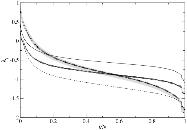
Figure 2: Lyapunov spectrum of the constant energy GNS system, approximated by 440 Fourier modes with $\langle\alpha\rangle=0.0105\pm 0.0006$ (plus symbols), and corresponding NS spectrum with $\nu=0.011$ (cross symbols). For clarity, only one third of the symbols are drawn and the shaded regions around them correspond to the errors, which are estimated as the range between the highest and lowest computed value, in the last two thirds of the run. The upper and lower thin lines concern the NS system with $\nu=0.007$ (solid) and $\nu=0.015$ (dashed), which are well below and above $\langle\alpha\rangle$ (error bars have the same size as for $\nu=0.011$).

4 The mathematical theory

The mathematical approach of Gallavotti and Cohen, [32, 33], is meant to identify the context within which a relation like Eq.(1) can be rigorously derived, i.e. to place on solid mathematical grounds the Lyapunov weights used in [29]. This approach assumes that dissipative, reversible, transitive Anosov diffeomorphisms are idealizations of nonequilibrium particle systems, hence that the statistical properties of Anosov and particle systems have some similarity. That systems evolve with discrete or continuous time, was considered a side issue in [32, 33], as apparently confirmed by Gentile’s work on Anosov flows [118].

We now sketch the derivation of the $\Lambda$-FR of [32, 33]. Take a smooth compact manifold $\mathcal{M}$, with a Riemann metric, and a diffeomorphism on it, $S:\mathcal{M}\to\mathcal{M}$, with Hölder continuous first derivatives. The dynamical system $(\mathcal{M},S)$ is Anosov if $\mathcal{M}$ is uniformly hyperbolic for $S$: i.e. there is a splitting of the tangent bundle $T\mathcal{M}=V^{-}\oplus V^{+}$, such that $x\mapsto V^{\pm}_{x}$ is Hölder continuous, $TS~{}V^{-}\subset V^{-}$, $TS~{}V^{+}=V^{+}$, and

$$\|TS^{n}v\|\leq C\theta^{-n}\quad\mbox{ for }v\in V^{-}$$ (24)

$$\|TS^{-n}v\|\leq C\theta^{-n}\quad\mbox{ for }v\in V^{+}$$ (25)

for all $n\geq 0$ and for given constants $C>0$, $\theta>1$. The dynamics is transitive if the stable and unstable manifolds $V^{\pm}_{x}$ are dense in $\mathcal{M}$ for all $x\in\mathcal{M}$. The following holds [119]:

Theorem (Sinai, 1968). Every transitive Anosov diffeomorphism has a Markov partition.

A Markov partition is a subdivision of $\mathcal{M}$ in cells whose interiors are disjoint from each other, and whose boundaries are invariant sets constructed using the stable and unstable manifolds. This allows the interior of a cell to be mapped by $S$ in the interior of other cells, and not across two cells, which would include a piece of their boundary. Furthermore, partitions with arbitrarily small cells can be constructed. Now, let $J$ be the Jacobian determinant of $S$, $\Lambda(x)=-\log J(x)$, and consider the dimensionless phase space contraction rate averaged on a trajectory segment $w_{x,\tau}$ of middle point $x\in\mathcal{M}$, and duration $\tau$:

$$e_{\tau}(x)=\frac{1}{\tau\langle\Lambda\rangle}\sum_{-\tau/2}^{\tau/2-1}\Lambda(S^{t}x)$$ (26)

Let $J^{u}$ be the Jacobian determinant of $S$ restricted to $V^{+}$. If the system is Anosov, probability weights of the kind conjectured in [29] can be assigned to the cells of a finite Markov partition, and the probability that $e_{\tau}(x)$ falls in the interval $B_{p,\epsilon}=(p-\epsilon,p+\epsilon)$ coincides, in the limit of fine Markov partitions and long $\tau$’s, with the sum of the weights $w_{x,\tau}=\Pi_{k=-\tau/2}^{\tau/2-1}J^{u}(S^{k}x)^{-1}$ of the cells containing the points $x$ with $e_{\tau}(x)\in B_{p,\epsilon}$. Then, if $\pi_{\tau}(B_{p,\epsilon})$ is the corresponding probability, one can write

$$\pi_{\tau}(B_{p,\epsilon})\approx\frac{1}{M}\sum_{x,e_{\tau}(x)\in B_{p,\epsilon}}w_{x,\tau}$$ (27)

where $M$ is a normalization constant. If the support of the physical measure is $\mathcal{M}$, which is the case if the dissipation is not exceedingly high [120], time reversibility guarantees that the support of $\pi_{\tau}$ is symmetric around $0$, and one can consider the ratio

$$\frac{\pi_{\tau}(B_{p,\epsilon})}{\pi_{\tau}(B_{-p,\epsilon})}\approx\frac{\sum_{x,e_{\tau}(x)\in B_{p,\epsilon}}w_{x,\tau}}{\sum_{x,e_{\tau}(x)\in B_{-p,\epsilon}}w_{x,\tau}}~{},$$ (28)

where each $x$ in the numerator has a counterpart in the denominator. Denoting by $i$ the involution which replaces the initial condition of one trajectory with the initial condition of the reversed trajectory, time reversibility yields:

$$\Lambda(x)=-\Lambda(ix)~{},\quad w_{ix,\tau}=w_{x,\tau}^{-1}\quad\mbox{and~{}~{}~{} }\frac{w_{ix,\tau}}{w_{x,\tau}}=\exp(\tau\langle\Lambda\rangle p)$$ (29)

if $e_{\tau}(x)=p$. Taking small $\epsilon$ in $B_{p,\epsilon}$, the division of each term in the numerator of (28) by its counterpart in the denominator approximately equals $e^{\tau\langle\Lambda\rangle p}$, which then equals the ratio in (28). In the limit of small $\epsilon$, infinitely fine Markov partition and large $\tau$ one obtains:

Theorem (Gallavotti and Cohen, 1995). Let $(\mathcal{M},S)$ be dissipative, reversible and chaotic. Then,

$$\frac{\pi_{\tau}(B_{p,\epsilon})}{\pi_{\tau}(B_{-p,\epsilon})}=e^{\tau\langle\Lambda\rangle p}~{}.$$ (30)

with an error in the argument of the exponential which can be estimated to be $p,\tau$ independent.

Here, dissipative means $\langle\Lambda\rangle>0$; reversible means $iS^{n}=S^{-n}i$; and chaotic means that $S$ can be regarded as a transitive Anosov system for the purpose of computing its statistical properties (Chaotic Hypothesis, Sec. 2). If $\Lambda$ can be identified with a physical observable, the $\Lambda$-FR is a statement on the physics of nonequilibrium systems.

A quite informative derivation of the $\Lambda$-FR is the one based on orbital measures, given by Ruelle in Ref.[121], which we now summarize. Take a transitive, reversible Anosov diffeomorphism described above, and a Hölder continuous function $A:\mathcal{M}\to I\hskip-3.4ptR$; there is a unique ergodic measure $\mu$ maximizing $h(\mu)+\int A(x)\mu(dx)$, where $h$ is the Kolmogorov-Sinai entropy and $\mu$ is called the Gibbs state for $A$. Sinai proved that the invariant measure which gives the forward time statistics is the Gibbs state of $A=-\log J^{u}$. Denoting by Fix$S^{n}=\{x\in\mathcal{M}:S^{n}x=x\}$, the set of periodic points of period $n$ and by $\phi$ a continuous function, the probability measure $\mu_{n}$ defined by the averages

$$\mu_{n}(\phi)=\frac{\sum_{\mbox{Fix}S^{n}}\phi(x)\Pi_{k=0}^{n-1}J^{u}(S^{k}x)^{-1}}{\sum_{\mbox{Fix}S^{n}}\Pi_{k=0}^{n-1}J^{u}(S^{k}x)^{-1}}$$ (31)

is invariant for $S$ and tends weakly to $\mu$ for $n\to\infty$: $\mu_{n}(\phi)\to\mu(\phi)$ for all $\phi$. Moreover, by definition $\mu(e_{\tau})=1$ and, because of time reversibility, one has

$$J(iSx)=J(x)^{-1}~{},\quad e_{\tau}\circ i\circ S^{\tau}=-e_{\tau}~{},\quad\mbox{and ~{}~{}~{}}~{}~{}~{}J^{s}(iSx)=J^{u}(x)^{-1}$$ (32)

since $i$ exchanges the stable and unstable directions. To prove the $\Lambda$-FR , observe first that, given $[p,q]\subset I\hskip-3.4ptR$, there are $a,b>0$ for which

$$\frac{1}{\tau\langle\Lambda\rangle}\log\frac{\mu(x:e_{\tau}(x)\in[p,q])}{\mu(x:e_{\tau}(x)\in[-q-a/\tau,-p+a/\tau])}\leq q+\frac{b}{\tau}~{}.$$ (33)

This rather sophisticated result was obtained by Ruelle relying heavily on properties of Anosov diffeomorphisms, hence it should hardly be generic (see also [122]). Indeed, Eq.(33) relies on Bowen’s shadowing, topologically mixing, the specification property, a property of sums for Hölder continuous functions, the expansiveness of the dynamics, the continuity of the splitting of the tangent bundle, and the expression of $\mu$ in terms of periodic orbits (c.f., Sections 3.1 to 3.8 of Ref. [121]). Furthermore, Ruelle uses a large deviation result for one dimensional systems with short range interactions, considering $A=-\log J^{u}$ and $B=-(1/\langle\Lambda\rangle)\log J$, so that $(1/\tau)\sum_{k=0}^{\tau-1}B(S^{k}x)=e_{\tau}(x)$. This result states that there is a real analytic and strictly concave function $\eta$ in the interval $(-p^{*},p^{*})$ such that, for every other interval $I$ which intersects $(-p^{*},p^{*})$, the following holds

$$\lim_{\tau\to\infty}\frac{1}{\tau\langle\Lambda\rangle}\log\mu\left(\left\{x:e_{\tau}(x)\in I\right\}\right)=\frac{1}{\langle\Lambda\rangle}\sup_{u\in I\cap(-p^{*},p^{*})}\eta(u)$$ (34)

where the Gibbs state of $A$, $\mu$, and time reversibility have been used. Combining this with (33), one obtains

$$\lim_{\tau\to\infty}\frac{1}{\tau\langle\Lambda\rangle}\log\frac{\mu(\{x:e_{\tau}(x)\in(p-\delta,p+\delta)\})}{\mu(\{x:e_{\tau}(x)\in(-p-\delta,-p+\delta)\})}\leq p+\delta$$ (35)

for $\delta>0$ and $|p|<p^{*}$. Taking this result, and the one corresponding to $-p$, the Gallavotti-Cohen fluctuation theorem is finally obtained.

Theorem (Ruelle, 1999). Let $S$ be a $C^{1+\alpha}$, $\alpha>0$, Anosov diffeomorphism of the compact connected manifold $\mathcal{M}$, and let $\mu$ be the corresponding SRB measure. Assume reversibility, with involution $i$, and consider the dimensionless phase space contraction rate $e_{\tau}$ with respect to an $i$-invariant Riemann metric on $\mathcal{M}$. Then, there exists $p^{*}>0$ such that the $\Lambda$-FR

$$p-\delta\leq\lim_{\tau\to\infty}\frac{1}{\tau\langle\Lambda\rangle}\log\frac{\mu(\{x:e_{\tau}(x)\in(p-\delta,p+\delta)\})}{\mu(\{x:e_{\tau}(x)\in(-p-\delta,-p+\delta)\})}\leq p+\delta$$ (36)

holds if $|p|<p^{*}$ and $\delta>0$.

4.1 Consequences of the $\Lambda$-FR

Taking $\Lambda$ as the entropy production rate, Gallavotti used the $\Lambda$-FR to obtain Green-Kubo like and Onsager like relations, in the limit of small dissipation [34]. This way, the $\Lambda$-FR appears as an extension of such relations to nonequilibrium systems. Gallavotti assumes that the (reversibly thermostatted, continuous time) system is driven by the $s$ fields $F=(F_{1},F_{2},...,F_{s})$, that $\Lambda$ vanishes for $F=0$, that the phase space is bounded, and that

$$\Lambda(x)=\sum_{i=1}^{s}F_{i}J_{i}^{0}(x)+O(F^{2})~{},$$ (37)

where $J_{i}^{0}$ are the currents close to equilibrium, i.e., are linear in $F$. Then, the fast decay of the $\Lambda$-autocorrelation function, implied by the Anosov property, leads to

$$\zeta(p)=-\lim_{\tau\to\infty}\frac{1}{\tau}\log\pi_{\tau}(p)=\frac{\langle\Lambda\rangle^{2}}{2C_{2}}(p-1)^{2}+O((p-1)^{3}F^{3})$$ (38)

where $C_{2}=\int_{-\infty}^{\infty}\langle\Lambda(S^{t}\cdot)\Lambda(\cdot)\rangle^{T}dt$, and $\langle.\rangle^{T}$ denotes the cumulant. Thus, using the $\Lambda$-FR, one obtains $\langle\Lambda\rangle=C_{2}/2+O(F^{3})$. Arbitrarily far from equilibrium, Gallavotti defines the currents as $J_{i}(x)=\partial_{F_{i}}\Lambda(x)$, and the transport coefficients as $L_{ij}=\partial_{F_{j}}\langle J_{i}\rangle|_{F=0}$. The derivatives with respect to the parameters $F$ require a property of differentiability of SRB measures, which has been proven by Ruelle in Ref.[28]. Assuming this property, the validity of the $\Lambda$-FR and using time reversibility, one can write $\partial_{F_{j}}\langle J_{i}^{0}\rangle|_{F=0}=\partial_{F_{j}}\langle J_{i}\rangle|_{F=0}$, and

$$\hskip-40.0pt\frac{1}{2}\int_{-\infty}^{\infty}\langle\Lambda(S^{t}x)\Lambda(x)\rangle^{T}dt=\langle\Lambda\rangle=\frac{1}{2}\sum_{i,j=1}^{s}(\partial_{F_{j}}\langle J_{i}\rangle+\partial_{F_{i}}\langle J_{j}\rangle)|_{F=0}F_{i}F_{j}~{},$$ (39)

in the limit of small $F$. Then, if $s=1$, one recovers the Green-Kubo relations for the unique transport coefficient $L_{11}$. To obtain the Onsager symmetry $L_{ij}=L_{ji}$, Gallavotti extends the $\Lambda$-FR in order to consider the joint distribution of $\Lambda$ and its derivatives. Introducing the dimensionless current $q$ in a trajectory segment

$$q(x)=\frac{1}{F_{j}\langle\partial_{F_{j}}\Lambda\rangle\tau}\int_{-\tau/2}^{\tau/2}F_{j}\partial_{F_{j}}\Lambda(S^{t}x)dt$$ (40)

and the joint distribution $\pi_{\tau}(p,q)$, with corresponding large deviation functional $\zeta(p,q)=-\lim_{\tau\to\infty}\frac{1}{\tau}\log\pi_{\tau}(p,q)$, one obtains a relation like the $\Lambda$-FR :

$$\lim_{\tau\to\infty}\frac{1}{\tau\langle\Lambda\rangle p}\log\frac{\pi_{\tau}(p,q)}{\pi_{\tau}(-p,-q)}=1~{}.$$ (41)

This makes the difference $(\zeta(p,q)-\zeta(-p,-q))$ independent of $q$, and leads to the desired result, $L_{ij}=L_{ji}$, in the limit of small $F$. This work inspired Refs.[35, 104, 105].

The above derivations are valid if the dynamics is transitive, i.e. if the dissipation is not too high. It is very hard to violate this condition in a particle system [120]. However, this possibility has been considered in [48], where a stronger hypothesis than the Chaotic Hypothesis has been introduced, under the assumption that the Lyapunov exponents come in pairs that sum to a constant $c<0$ [123, 124, 125], except for some pair of vanishing exponents. In Ref. [47], Bonetto et al. had conjectured that the $\Lambda$-FR should generalize to the form

$$\log\frac{\pi_{\tau}(B_{p,\epsilon})}{\pi_{\tau}(B_{-p,\epsilon})}=\tau\langle\Lambda_{r}\rangle\frac{D-M}{D}p\ ,$$ (42)

apart from small errors. To understand the meaning of $(D-M)/D\leq 1$ and $\Lambda_{r}$, consider transitive dynamics, and neglect the trivial Lyapunov exponents. Half of the remaining exponents are positive ($\lambda_{i}^{+}$), half are negative ($\lambda_{i}^{-}$), and can be arranged in $D$ pairs $\{\lambda_{i}^{+},\lambda_{i}^{-}\}$, with $c_{i}=\lambda_{i}^{+}+\lambda_{i}^{-}$. According to the authors of [47], as the dissipation grows, the dynamics ceases to be transitive, some of the positive exponents become negative and lower dimensional attracting and repelling sets are generated. If conjugate pairing holds, i.e. if $c_{i}=c$ for all $i=1,...,D$, it could happen that the volume contraction along each pair of directions corresponding to each pair of exponents is proportional to $c$, and that the dimensionality of the attracting manifold $\mathcal{M}_{r}$ is that of $\mathcal{M}$ minus the number $M$ of pairs with two negative exponents. Then, $\Lambda$ equals $(D-M)/D$ times the contraction rate restricted to the attractor, $\Lambda_{r}$ and, if the attractor is invariant with respect to some kind of time reversal operation, the FR holds for $\Lambda_{r}$, while $\Lambda$ must obey Eq.(42).

Eq.(42) is hard to test in particle systems, because fluctuations become less and less frequent as the dissipation grows. In Ref.[47], the case with $(D-M)/D=18/19$ was not distinguishable from 1, given the achieved resolution, while the case with $(D-M)/D=17/19$ could not be tested; similar difficulties were met in [61]. An indirect confirmation of Eq.(42), based however on new scaling assumptions, is given in [126], where a procedure is given to estimate finite $\tau$ corrections to the steady state $\Lambda$-FR. Differently, Ref.[50] finds that the standard $\Lambda$-FR holds for a simple oscillator model, even in the presence of pairs of negative Lyapunov exponents. The theory of Refs.[47, 48] has been generalized to hydrodynamic models, where conjugate pairing does not hold, but fluctuations persist even with a substantial excess of negative Lyapunov exponents [83, 84, 49]. The factor $(D-M)/D$ was there replaced by

$$c=\frac{\sum^{*}(\lambda_{k}+\lambda_{2K-1-k})}{\sum(\lambda_{k}+\lambda_{2K-1-k})}\ ,$$ (43)

where the $2K-2$ nontrivial Lyapunov exponents are given in decreasing order ($\lambda_{1}\geq\lambda_{2}...\geq\lambda_{2K-2}$), and $\sum^{*}$ means summation over the pairs with one positive exponent, while $\sum$ is the summation over all the pairs. The $\Lambda$-FR with slope $c$ defined by (43) was verified in GNS systems truncated to few tens of modes [49].

4.2 Local fluctuations

In Ref.[49] a local version of the $\Lambda$-FR, first proposed in [127], was also tested. One reason for developing local FRs is that global fluctuations are not observable in macroscopic systems. The local $\Lambda$-FR of Ref.[127] concerns an infinite chain of weakly interacting chaotic maps. Let $V_{0}$ be a finite region of the chain centered at the origin, $T_{0}>0$ be a time interval, and define

$$\langle\Lambda\rangle\equiv\lim_{V_{0},T_{0}\rightarrow\infty}\frac{1}{|V_{0}|T_{0}}\sum_{j=0}^{T_{0}-1}\Lambda_{V_{0}}(S^{j}x)~{},\quad p=\frac{1}{\langle\Lambda\rangle|V|}\sum_{j=-T_{0}/2}^{T_{0}/2}\Lambda_{V_{0}}(S^{j}x)~{},$$ (44)

where $V=V_{0}\times T_{0}$, and $\Lambda_{V_{0}}(x)$ is the contribution to $\Lambda$ given by $V_{0}$. Then, one obtains:

$$\pi_{V}(p)=e^{\zeta(p)|V|+O(|\partial V|)}~{},\quad\mbox{with }\frac{\zeta(p)-\zeta(-p)}{p\langle\Lambda\rangle}=1\quad\mbox{and }|p|<p^{*}~{},$$ (45)

where $|\partial V|$ is the size of the boundary of $V$, $p^{*}\geq 1$ and $\zeta$ is analytic in $p$. The contribution of the boundary term $|\partial V|$ decreases with growing $V$, leading to the $\Lambda$-FR in the limit of large (compared to microscopic scales) volume $V_{0}$ and long times $T_{0}$.

The problem of local fluctuations, naturally leads to the possibility of extending Onsager-Machlup theory to nonequilibrium systems. This has been done by Gallavotti [128], under the assumption that the entropy production rate is proportional to $\Lambda$. The Onsager-Machlup theory [13, 14] concerns the paths of small fluctuations around equilibrium states, and leads to a derivation of the hydrodynamic equations for the corresponding observables, via the maximization of the probability of the relaxation paths, in the large system limit [13, 14]. Gallavotti also considers the probability of temporal paths $t\mapsto\varphi(t)$, for observables $\mathcal{O}$ which are either even or odd with respect to the time reversal operation, and have vanishing mean. The fluctuation $\varphi$, is assumed to be smooth and to vanish for large $|t|$, but no bound is placed on its size. One may then consider the probability that $\mathcal{O}(S^{t}x)$ stays close to $\varphi$, in the time interval $[-\tau/2,\tau/2]$, and, in the large $\tau$ limit, one may consider the large deviation function for $\Lambda$ to take values close to $p$ and for $\mathcal{O}$ to stay close to $\varphi$, $\zeta(p,\varphi)$ say.

The result is that the path $\varphi(t)$ and its time reversal $i\varphi(t)=\pm\varphi(-t)$ (where $+$ holds for even and $-$ for odd $\varphi$) are followed with equal probability if the first path is conditioned to an average $\Lambda$ equal to $p$ and the second path to an average $\Lambda$ equal to $-p$. Indeed, for time reversal invariant, dissipative, transitive Anosov systems, Gallavotti obtains

$$\frac{\zeta(-p,i\varphi)-\zeta(p,\varphi)}{p\langle\Lambda\rangle}=1~{},\qquad|p|\leq p^{*}~{},\qquad p^{*}\geq 1~{},$$ (46)

which means that it suffices to make $\Lambda$ behave strangely (i.e.  to take values different from $\langle\Lambda\rangle$), to see all observables behave equally strangely. The further developments of Ref.[129] excluded a direct connection of these results with the theory of Ref.[82].

4.3 Applicability of the Chaotic Hypothesis

The question arises of whether any system of physical interest verifies the Chaotic Hypothesis. As the FR implied by the Chaotic Hypothesis concerns the physically non-obvious $\Lambda$, this question has been little investigated. Some of the papers in which $\Lambda$ was considered suggested that the steady state $\Lambda$-FR holds for reversible dynamical systems with one or more positive Lyapunov exponents [34], but also for some systems without positive exponents [130, 131]. That $\Lambda$ should be bounded and that the $\Lambda$-FR should hold only for $|p|\leq p^{*}$, for some $p^{*}>0$, was not thought to have observable consequences, at first.

Later it was realized that the $\Lambda$-FR is hard, if not impossible, to verify in non-isoenergetic systems in steady states close to equilibrium [57, 63, 60], despite the “higher chaos” of equilibrium states. To explain these facts, Ref.[36] observes that the $\Lambda$-FR implies an asymmetry between positive and negative fluctuations, which is not present in equilibrium, hence that the $\Lambda$-FR for non-normalized $\Lambda$ may hold only if its domain tends to $\{0\}$ when the steady state tends to an equilibrium state. In the Gaussian isokinetic case, however, $\Lambda$ is the sum of a dissipative term, $\Omega$, and a conservative interaction term, which may be singular, (cf.  Eqs. 8,11). The dissipative term obeys the FR, while the conservative term does not, but its averages over long time intervals are small, and become negligible with respect to those of $\Omega$ as the intervals grow [60, 36]. Thus, in the long time limit the $\Lambda$-FR may hold as a consequence of the validity of the $\Omega$-FR , but its convergence times diverge as the steady states approach equilibrium states. Moreover, the convergence of the domain of the $\Lambda$-FR to $\{0\}$ implies that the $\Lambda$-FR eventually describes only trivial fluctuations. This causes some difficulty in the derivation of the Green-Kubo relations from the $\Lambda$-FR, which requires the equilibrium limit. On the one hand, the averaging times have to be long for the Central Limit and the $\Lambda$-FR to apply, but not so long that $\Omega=0$ is in the tails of the $\Omega$-probability distribution function, which are not described by the Central Limit Theorem. If the averaging time required by the $\Lambda$-FR tends to infinity, this compromise may not be possible. Singularities of $\Lambda$, in turn, make dubious the existence of the cumulants used in [34] to derive the Green-Kubo relations. Therefore, the physical applications of the $\Lambda$-FR and of the Chaotic Hypothesis appear problematic from this point of view.

References [36, 132] suggested that, in IK systems, $\Lambda$ is better suited to describe heat fluxes than entropy productions, hence that the $\Lambda$-FR has to be modified like the heat FR of Van Zon and Cohen for stochastic systems [133]. Indeed, for continuous time systems with singular $\Lambda$, terms of the form $[\Phi^{int}(S^{\tau}x)-\Phi^{int}(x)]/\tau$, with unbounded interaction potential ${\Phi}^{int}$, affect the large deviations of $\Lambda$, if the probability distribution of $\Phi^{int}$ has exponential or larger tails [134]. The solution of Ref.[134] consists in assuming that chaos due to uniform hyperbolicity may play the same role as the white noise in Ref.[79, 80]. In the Gaussian isokinetic, or Nosé-Hoover isothermal cases, one has

$$\dot{{\bf q}}_{i}={\bf p}_{i}\qquad\dot{{\bf p}}_{i}=E-\partial_{{\bf q}_{i}}\Phi^{int}-\alpha{\bf p}_{i}\qquad\Lambda=\Lambda^{(0)}-\beta\dot{V}$$ (47)

where $V$ is related to $\Phi^{int}$, and has an equilibrium ($E=0$) distribution with exponentially decaying tails, while $\Lambda^{(0)}$ has Gaussian tails. It is then assumed that the tails have same properties when $E\neq 0$. Then, the average of $\Lambda$ in a time $\tau$ takes the form

$$\overline{\Lambda}_{0,\tau}(x)=\frac{1}{\tau}\int_{0}^{\tau}\Lambda(S^{t}x)dt=\overline{\Lambda^{(0)}}_{0,\tau}(x)+\frac{\beta}{\tau}\left[V(S^{\tau}x)-V(x)\right]~{},$$ (48)

with $$\overline{\Lambda^{(0)}}_{0,\tau}(x)=\frac{1}{\tau}\int_{0}^{\tau}\Lambda^{(0)}(S^{t}x)dt\ ,$$ (49)

and for large $\tau$, in some cases, one may assume that $\Lambda^{(0)}$, $V_{f}=V\circ S^{\tau}$ and $V_{i}=V$ are independently distributed. This ultimately leads to [134]

$$\hskip-50.0pt\lim_{\tau\to\infty}\frac{1}{\tau}\log\int_{-p^{*}\langle\Lambda\rangle}^{p^{*}\langle\Lambda\rangle}d\Lambda^{(0)}\int_{0}^{\infty}dV_{i}\int_{0}^{\infty}dV_{f}e^{\tau\tilde{\zeta}_{0}(\Lambda^{(0)})-\beta(V_{i}+V_{f})}\delta[\tau(\Lambda-\Lambda^{(0)})+\beta(V_{i}-V_{f})]$$ (50)

$$=\lim_{\tau\to\infty}\frac{1}{\tau}\log\int_{-p^{*}\langle\Lambda\rangle}^{p^{*}\langle\Lambda\rangle}d\Lambda^{(0)}e^{\tau\tilde{\zeta}_{0}(\Lambda^{(0)})-\tau|\Lambda-\Lambda^{(0)}|}\ ,$$ (51)

where $\tilde{\zeta}_{0}(\Lambda^{(0)})$ is the rate function of $\Lambda^{(0)}$. Then, for the rate function of $\Lambda$ one obtains

$$\hskip-60.0pt\tilde{\zeta}(\Lambda)=\max_{\Lambda^{(0)}\in[-p^{*}\langle\Lambda\rangle,p^{*}\langle\Lambda\rangle]}\left[\tilde{\zeta}_{0}(\Lambda^{(0)})-|\Lambda-\Lambda^{(0)}|\right]=\left\{\begin{array}[]{lll}\tilde{\zeta}_{0}(\Lambda_{-})-\Lambda_{-}+\Lambda&;&\Lambda<\Lambda_{-}\\ \tilde{\zeta}_{0}(\Lambda)&;&\Lambda_{-}\leq\Lambda\leq\Lambda_{+}\\ \tilde{\zeta}_{0}(\Lambda_{+})+\Lambda_{+}-\Lambda&;&\Lambda>\Lambda_{+}\end{array}\right.$$ (52)

where $\tilde{\zeta}_{0}^{\prime}(\Lambda_{\pm})=\mp 1$. If the FR holds for $\Lambda^{(0)}$, with $|\Lambda^{(0)}|\leq p^{*}\langle\Lambda\rangle$, the $\Lambda^{(0)}$-FR, one obtains

$$\tilde{\zeta}(\Lambda)-\tilde{\zeta}(-\Lambda)=\left\{\begin{array}[]{lll}\Lambda&;&0\leq\Lambda<\langle\Lambda\rangle\\ \tilde{\zeta}_{0}(\Lambda)+\Lambda&;&\langle\Lambda\rangle\leq\Lambda\leq\Lambda_{+}\\ \tilde{\zeta}_{0}(\Lambda_{+})+\Lambda_{+}&;&\Lambda>\Lambda_{+}\end{array}\right.\ .$$ (53)

A relation similar to the heat FR of Van Zon and Cohen is thus obtained for $\Lambda$. The statement that the $\Lambda^{(0)}$-FR holds with $|p|\leq p^{*}$, if $\Lambda^{(0)}$ is bounded or decays faster than exponential is justified adopting Gentile’s approach for Anosov flows, which reduces the flow to a Poincaré map [118], and assuming the Chaotic Hypothesis for the resulting map. In particular, the dynamics may be restricted to a level surface $V=\bar{V}$, with $\bar{V}<\infty$, so that the volume contraction rate, $\Lambda^{(0)}$, is bounded and the terms $(V_{f}-V_{i})$ vanish.

This scenario is supported by Gilbert’s Ref.[67], for a one particle system. However, all other particle systems have been found to satisfy the original $\Lambda$-FR, suggesting that the singularities in the potential term may not be sufficient for the validity of the heat FR of Van Zon and Cohen [135]. For stochastic systems, the first indication that singularities may invalidate the $\Lambda$-FR is found in [136]; Ref.[137] suggests that the Van Zon-Cohen FR may have quite wide applicability, see also [138], while [139] shows some counterexample. The phenomenology is quite complex, as Visco explains [140], hence it is not possible at present to draw the limits of validity of the theory of [134].

The above shows that the $\Lambda$-FR rests on strong assumptions, which are hardly met by systems of physical interest, and which have no simple physical interpretation. At the same time, the physically more obvious steady state $\Omega$-FR is quite generally verified, and does not incur in the difficulties which affect the $\Lambda$-FR. Thus the mathematical theory raises intriguing questions for the physical theory: does the $\Omega$-FR hold independently of the $\Lambda$-FR? Which are the physical mechanisms underlying the validity of the $\Omega$-FR, when it holds? It would also be interesting to test Eqs.(41,46) in NEMD models, as well as in actual experiments, and it is desirable that Eqs.(42,45,53) be further investigated.

5 The physical mechanisms

In 1994, Evans and Searles obtained the first of a series of relations similar to Eq.(1), for the Dissipation Function $\Omega$, which, in nonequilibrium states close to equilibrium can be identified with the entropy production rate, $\sigma=JVF^{ext}/k_{{}_{B}}T$. Here, $J$ is the (intensive) flux due to the thermodynamic force $F^{ext}$, $V$ is the volume and $T$ the kinetic temperature [30, 31]. That relation, called transient $\Omega$-FR, is obtained under virtually no hypothesis, except for time reversibility; it is transient because it concerns non-invariant ensembles of systems, instead of the steady state. The transient $\Omega$-FR has been verified experimentally [141, 64, 65], and its conjectured extension to steady states has been validated by many tests. The Evans-Searles approach to the steady state $\Omega$-FR is based on the belief that the complete knowledge of the invariant measure implied by the Chaotic Hypothesis is not needed to understand a few properties of the steady state. Like thermodynamic relations are widely applicable because do not depend on the details of the microscopic dynamics, the observed wide applicability of the steady state $\Omega$-FR suggests, indeed, that it cannot depend on subtle dynamical features, like approximate hyperbolicity. It is therefore necessary to understand the mechanisms underlying the validity of the steady state $\Omega$-FR in systems of physical interest.

Following Ref.[46], let ${\cal M}$ be the phase space of the system at hand, and $S^{\tau}:{\cal M}\rightarrow{\cal M}$, a reversible evolution with time reversal map $i$. Take a probability measure $d\mu({\Gamma})=f({\Gamma})d{\Gamma}$ on ${\cal M}$, and let the observable $\mathcal{O}:{\cal M}\rightarrow I\hskip-3.4ptR$ be odd with respect to time reversal i.e.,  $\mathcal{O}(i{\Gamma})=-\mathcal{O}({\Gamma})$. Denote its time averages by

$$\overline{\mathcal{O}}_{t_{0},t_{0}+\tau}({\Gamma})\equiv\frac{1}{\tau}\mathcal{O}_{t_{0},t_{0}+\tau}({\Gamma})=\frac{1}{\tau}\int_{t_{0}}^{t_{0}+\tau}\mathcal{O}(S^{s}{\Gamma})ds~{}.$$ (54)

For a density $f$ even with respect to time reversal, i.e. satisfying $f(i{\Gamma})=f({\Gamma})$, define the Dissipation Function as

$$\hskip-65.0pt\Omega({\Gamma})=-\left.\frac{d}{d{\Gamma}}\log f\right|_{\Gamma}\cdot\dot{{\Gamma}}+\Lambda({\Gamma})~{},\quad\mbox{so that}~{}~{}~{}\overline{\Omega}_{t_{0},t_{0}+\tau}({\Gamma})=\frac{1}{\tau}\left[\ln\frac{f(S^{t_{0}}{\Gamma})}{f(S^{t_{0}+\tau}{\Gamma})}+\Lambda_{t_{0},t_{0}+\tau}\right]$$ (55)

Note that, for a compact phase space, the uniform density $f({\Gamma})=1/|{\cal M}|$ implies $\Omega=\Lambda$. However, $\Omega$ equals the dissipated power, divided by the kinetic temperature, in bulk thermostatted systems, like those of Eqs.(7), only if $f$ is the equilibrium probability density for the given system [46], and only in special circumstances does this imply $f({\Gamma})=1/|{\cal M}|$. That the logarithmic term exists in (55) has been called ergodic consistency [51], a condition met if $f>0$ in all regions visited by the trajectories $S^{t}{\Gamma}$.

For $\delta>0$, let $A^{+}_{\delta}=(A-\delta,A+\delta)$ and $A^{-}_{\delta}=(-A-\delta,-A+\delta)$, and let $E(\mathcal{O}\in(a,b))$ be the set of points ${\Gamma}$ such that $\mathcal{O}({\Gamma})\in(a,b)$. Then, $E(\overline{\Omega}_{0,\tau}\in A^{-}_{\delta})=iS^{\tau}E(\overline{\Omega}_{0,\tau}\in A^{+}_{\delta})$, and the transformation ${\Gamma}=iS^{\tau}X$ has Jacobian

$$\left|\frac{d{\Gamma}}{dX}\right|=\exp\left(-\int_{0}^{\tau}\Lambda(S^{s}X)ds\right)=e^{-\Lambda_{0,\tau}(X)}~{},$$ (56)

Then, introducing $\left\langle\mathcal{O}\right\rangle_{\overline{\Omega}_{0,\tau}\in A^{+}_{\delta}}$ as the average of $\mathcal{O}$ according to $\mu$, under the condition that $\overline{\Omega}_{0,\tau}\in A^{+}_{\delta}$, and taking the dissipation function as the observable, $\overline{\mathcal{O}}_{0,\tau}=\overline{\Omega}_{0,\tau}$, one may write

$$\frac{\mu(E(\overline{\Omega}_{0,\tau}\in A^{+}_{\delta}))}{\mu(E(\overline{\Omega}_{0,\tau}\in A^{-}_{\delta}))} = \frac{\int_{E(\overline{\Omega}_{0,\tau}\in A^{+}_{\delta})}f({\Gamma})d{\Gamma}}{\int_{E(\overline{\Omega}_{0,\tau}\in A^{+}_{\delta})}f(S^{\tau}X)e^{-\Lambda_{0,\tau}(X)}dX}$$ (57)

$$= \frac{\int_{E(\overline{\Omega}_{0,\tau}\in A^{+}_{\delta})}f({\Gamma})d{\Gamma}}{\int_{E(\overline{\Omega}_{0,\tau}\in A^{+}_{\delta})}e^{-\Omega_{0,\tau}(X)}f(X)dX}=\left\langle e^{-\Omega_{0,\tau}}\right\rangle_{\overline{\Omega}_{0,\tau}\in A^{+}_{\delta}}^{-1}\ ,$$

i.e.,

$$\frac{\mu(E(\overline{\Omega}_{0,\tau}\in A^{+}_{\delta}))}{\mu(E(\overline{\Omega}_{0,\tau}\in A^{-}_{\delta}))}=e^{[A+\epsilon(\delta,A,\tau)]\tau}\ ,$$ (58)

with $\epsilon$ an error term due to the finiteness of $\delta$, such that $|\epsilon(\delta,A,\tau)|\leq\delta$. We call (58) the transient $\Omega$-FR. The transient $\Omega$-FR refers to the non-invariant probability measure $\mu$ of density $f$; it is remarkable that time reversibility is the only ingredient of its derivation. To obtain the steady state $\Omega$-FR, let averaging begin at time $t_{0}$ and consider

$$\frac{\mu(E(\overline{\mathcal{O}}_{t_{0},t_{0}+\tau}\in A^{+}_{\delta}))}{\mu(E(\overline{\mathcal{O}}_{t_{0},t_{0}+\tau}\in A^{-}_{\delta}))}\ .$$ (59)

Taking $t=\tau+2t_{0}$, the transformation ${\Gamma}=iS^{t}W$ and some algebra yield

$$\frac{\mu(E(\overline{\mathcal{O}}_{t_{0},t_{0}+\tau}\in A^{+}_{\delta}))}{\mu(E(\overline{\mathcal{O}}_{t_{0},t_{0}+\tau}\in A^{-}_{\delta}))}=\left\langle\exp\left(-\Omega_{0,t}\right)\right\rangle_{\overline{\mathcal{O}}_{t_{0},t_{0}+\tau}\in A^{+}_{\delta}}^{-1}\ ,$$ (60)

and for $\overline{\mathcal{O}}_{t_{0},t_{0}+\tau}=\overline{\Omega}_{t_{0},t_{0}+\tau}$

$$\frac{\mu(E(\overline{\Omega}_{t_{0},t_{0}+\tau}\in A^{+}_{\delta}))}{\mu(E(\overline{\Omega}_{t_{0},t_{0}+\tau}\in A^{-}_{\delta}))}=e^{\left[A+\epsilon(\delta,t_{0},A,\tau)\right]\tau}\left\langle e^{-\Omega_{0,t_{0}}-\Omega_{t_{0}+\tau,2t_{0}+\tau}}\right\rangle_{\overline{\Omega}_{t_{0},t_{0}+\tau}\in A^{+}_{\delta}}^{-1}\ ,$$ (61)

where $|\epsilon(\delta,t_{0},A,\tau)|\leq\delta$ is due to the finiteness of $A^{+}_{\delta}$.

Having fixed $\tau>0$ and the tolerance $\delta>0$, we say that $A$ lies in the domain $\mathcal{D}$ of the steady state $\Omega$-FR, if there exists $\hat{t}>0$ such that $\mu(E(\overline{\Omega}_{t_{0},t_{0}+\tau}\in A^{+}_{\delta}))>0$ and $\mu(E(\overline{\Omega}_{t_{0},t_{0}+\tau}\in A^{-}_{\delta}))>0$ for all $t_{0}\geq\hat{t}$. In other words, $A\in\mathcal{D}$ if positive and negative fluctuations of size $A$ have positive probability in the steady state. Using $\mu(E)=\mu_{t_{0}}(S^{t_{0}}E)$, where $E$ is a subset of ${\cal M}$, and $\mu_{t_{0}}$ is the evolved measure up to time $t_{0}$, with density $f_{t_{0}}$, some algebra yields the $\mathcal{O}$-FR:

$$\frac{\mu_{{t_{0}}}(E(\overline{\mathcal{O}}_{0,\tau}\in A^{+}_{\delta}))}{\mu_{{t_{0}}}(E(\overline{\mathcal{O}}_{0,\tau}\in A^{-}_{\delta}))}=\frac{\mu(E(\overline{\mathcal{O}}_{t_{0},t_{0}+\tau}\in A^{+}_{\delta}))}{\mu(E(\overline{\mathcal{O}}_{t_{0},t_{0}+\tau}\in A^{-}_{\delta}))}=\langle\exp\left(-\Omega_{0,t}\right)\rangle^{-1}_{\overline{\mathcal{O}}_{t_{0},t_{0}+\tau}\in A^{+}_{\delta}}\ .$$ (62)

For $\overline{\mathcal{O}}_{t_{0},t_{0}+\tau}=\overline{\Omega}_{t_{0},t_{0}+\tau}$, taking the logarithm and dividing by $\tau$ produces:

$$\hskip-40.0pt\frac{1}{\tau}\ln\frac{\mu_{t_{0}}(E(\overline{\Omega}_{0,\tau}\in A^{+}_{\delta}))}{\mu_{t_{0}}(E(\overline{\Omega}_{0,\tau}\in A^{-}_{\delta}))}=A+\epsilon(\delta,t_{0},A,\tau)-\frac{1}{\tau}\ln\left\langle e^{-\Omega_{0,t_{0}}-\Omega_{t_{0}+\tau,2t_{0}+\tau}}\right\rangle_{\overline{\Omega}_{t_{0},t_{0}+\tau}\in A^{+}_{\delta}}$$ (63)

If $\mu_{t_{0}}$ tends to a steady state $\mu_{\infty}$ when $t_{0}\to\infty$, Eq.(63) should change from a statement on the ensemble $f_{t_{0}}$, to a statement on the statistics generated by a single typical trajectory. To be of practical use, however, this statement requires that the logarithm of the conditional average, divided by $\tau$, $M(A,\delta,t_{0},\tau)$ say, be controllable in Eq.(63). For instance, if it can be made negligible, e.g. letting $\delta$ be small and $\tau$ grow after the $t_{0}\to\infty$ limit has been taken, as in the case of the $\Lambda$-FR, one would have the

Steady State $\Omega$-FR. For any tolerance $\gamma>0$ and $A\in\mathcal{D}$, there are sufficiently small $\delta>0$ and large $\tau$, such that

$$A-\gamma\leq\frac{1}{\tau}\ln\frac{\mu_{\infty}(E(\overline{\Omega}_{0,\tau}\in A^{+}_{\delta}))}{\mu_{\infty}(E(\overline{\Omega}_{0,\tau}\in A^{-}_{\delta}))}\leq A+\gamma$$ (64)

holds.

As in the case of the $\Lambda$-FR, the domain $\mathcal{D}$ would be model dependent, and its expression could rest on non-trivial dynamical relations [68]. This requires some assumption. Indeed, the growth of $t_{0}$ could make $M(A,\delta,t_{0},\tau)$ diverge (as in properly devised examples [46]). If $\lim_{t_{0}\to\infty}|M(A,\delta,t_{0},\tau)|$ is bounded by some finite $M(A,\delta,\tau)$, $\lim_{\tau\to\infty}M(A,\delta,\tau)$ could still exceed the value of $\gamma$. The first difficulty is simply solved by the observation that the divergence of $M(A,\delta,t_{0},\tau)$ implies a divergence of the left hand side of Eq.(63), which in turn means that one of its two probabilities vanish, i.e. that $A\notin\mathcal{D}$. If $\mathcal{D}$ is empty, the steady state $\Omega$-FR is of no interest, because there are no fluctuations in the steady state.

Therefore, let us assume that $A\in\mathcal{D}$, and observe that the conservation of probability yields the relation

$$\left\langle e^{-\Omega_{0,s}}\right\rangle=1~{},\quad\mbox{for every }s\in I\hskip-3.4ptR~{},$$ (65)

first derived by Morriss and Evans (cf. [53], pp.198-202). Then, one possibility that can be considered is that the $\Omega$-autocorrelation time vanishes. In that case, one can write:

$$1=\left\langle e^{-\Omega_{0,s}-\Omega_{s,t}}\right\rangle=\left\langle e^{-\Omega_{0,s}}\right\rangle\left\langle e^{-\Omega_{s,t}}\right\rangle~{},\quad\left\langle e^{-\Omega_{s,t}}\right\rangle=1~{},\quad\mbox{for all}~{}s,t~{},$$ (66)

hence

$$\hskip-40.0pt\left\langle e^{-\Omega_{0,t_{0}}}\cdot e^{-\Omega_{t_{0}+\tau,2t_{0}+\tau}}\right\rangle_{\overline{\Omega}_{t_{0},t_{0}+\tau}\in A^{+}_{\delta}}=\left\langle e^{-\Omega_{0,t_{0}}}\cdot e^{-\Omega_{t_{0}+\tau,2t_{0}+\tau}}\right\rangle=1~{}.$$ (67)

Then, the logarithmic correction term in (63) identically vanishes for all $t_{0},\tau$, and the $\Omega$-FR is verified at all $\tau>0$. Of course, this idealized situation does not need to be realized, but tests performed on molecular dynamics systems [142] indicate that the typical situation is not dissimilar from this; typically, there exists a constant $K$, such that

$$0<\frac{1}{K}\leq\left\langle e^{-\Omega_{0,t_{0}}-\Omega_{t_{0}+\tau,2t_{0}+\tau}}\right\rangle_{\overline{\Omega}_{t_{0},t_{0}+\tau}\in A^{+}_{\delta}}\leq K~{}.$$ (68)

As a matter of fact, the de-correlation or Maxwell time, $t_{M}$, expresses a physical property of the system, thus it does not depend on $t_{0}$ or $\tau$, and depends only mildly on the external field [usually, $t_{M}(F_{e})=t_{M}(0)+O(F_{e}^{2})$]. Its order of magnitude is that of the mean free time. If $\tau\gg t_{M}$, the boundary terms $\Omega_{t_{0}-t_{M},t_{0}}$ and $\Omega_{t_{0}+\tau,t_{0}+\tau+t_{M}}$ are typically small compared to $\Omega_{t_{0},t_{0}+\tau}$, unless some singularity of $\Omega$ occurs within $(t_{0}-t_{M},t_{0})$ or $(t_{0}+\tau,t_{0}+\tau+t_{M})$. However, similar events may equally occur in the intervals $(0,t_{0})$ and $(t_{0}+\tau,2t_{0}+\tau)$, hence $\Omega_{t_{0}-t_{M},t_{0}}$ and $\Omega_{t_{0}+\tau,t_{0}+\tau+t_{M}}$ are expected to contribute only a fraction of order $O(t_{M}/\tau)$ to the arguments of the exponentials in the conditional average. Therefore, one can write

$$\hskip-50.0pt\left\langle e^{-\Omega_{0,t_{0}}}\cdot e^{-\Omega_{t_{0}+\tau,2t_{0}+\tau}}\right\rangle_{\overline{\Omega}_{t_{0},t_{0}+\tau}\in A_{\delta}^{+}} \approx \left\langle e^{-\Omega_{0,t_{0}-t_{M}}}\cdot e^{-\Omega_{t_{0}+\tau+t_{M},2t_{0}+\tau}}\right\rangle_{\overline{\Omega}_{t_{0},t_{0}+\tau}\in A_{\delta}^{+}}$$ (69)

$$\approx \left\langle e^{-\Omega_{0,t_{0}-t_{M}}}\cdot e^{-\Omega_{t_{0}+\tau+t_{M},2t_{0}+\tau}}\right\rangle$$

$$\approx \left\langle e^{-\Omega_{0,t_{0}+t_{M}}}\right\rangle\left\langle e^{-\Omega_{t_{0}+\tau+t_{M},2t_{0}+\tau}}\right\rangle=O(1)\ ,$$

with an accuracy which improves with growing $t_{0}$ and $\tau$, because $t_{M}$ is fixed. If these scenarios are realized, Eq.(68) follows and $M(A,\delta,t_{0},\tau)$ vanishes as $1/\tau$, with a characteristic scale of order $O(t_{M})$. In summary, the steady state $\Omega$-FR holds under the following conditions.

Conditions:
1. the dynamics is time reversal invariant.
2. $\mu_{t}$ tends to $\mu_{\infty}$ for $t\to\infty$.
3. Eq.(68) is satisfied with $K>0$, for $A\in\mathcal{D}$, if $\tau$ and $t_{0}$ are sufficiently larger than $t_{M}$.

Condition (68) can actually be weakened, but the decay of the $\Omega$-autocorrelations characterizes the convergence to a steady state, and is very widely verified. Therefore, the validity of Eq.(68), and not a weaker condition, explains why the steady state $\Omega$-FR holds for the particle systems so far investigated. The above derivation of the steady state $\Omega$-FR, under Conditions 1, 2 and 3, will not only answer the physics questions, but will also be mathematically rigorous, if it will be proven that one (possibly physically uninteresting) dynamical system satisfies them.

Various other relations can now be obtained [46]. For instance, any odd $\mathcal{O}$, any $\delta>0$, any $t_{0}$ and any $\tau$ yield

$$\langle\exp\left(-\Omega_{0,t}\right)\rangle_{\overline{\mathcal{O}}_{t_{0},t_{0}+\tau}\in(-\delta,\delta)}=\frac{\mu_{t_{0}}(E(\overline{\mathcal{O}}_{0,\tau}\in(-\delta,\delta)))}{\mu_{t_{0}}(E(\overline{\mathcal{O}}_{0,\tau}\in(-\delta,\delta)))}=1\ ,$$ (70)

which, in the $\delta\to\infty$ limit, produces the normalization property (65). The Dissipation relation

$$\langle\mathcal{O}\rangle_{t}=\int_{0}^{t}ds\langle\Omega(0)\mathcal{O}(s)\rangle$$ (71)

is another direct consequence of the approach followed in this section [143].

5.1 Green-Kubo relations

A consistency check of the present theory is afforded by the derivation of the Green-Kubo relations based on the $\Omega$-FR [36]. Differently from Ref.[34], which deals with time-asymptotic quantities, this derivation stresses the role of the physical time scales. To be concrete, take a Nosé-Hoover thermostatted system, whose equilibrium state is the extended canonical density

$$f_{c}(x,\alpha)=\frac{e^{-\beta\left(H_{0}+Q\alpha^{2}/2\right)}}{\int d\alpha~{}dx~{}~{}e^{-\beta\left(H_{0}+Q\alpha^{2}/2\right)}}\ ,$$ (72)

where $Q=2K_{0}\tau^{2}$ and $H_{0}$ is the internal energy [53]. This yields

$$f_{c}(\alpha)=\int dxf_{c}(x,\alpha)=\sqrt{\frac{\beta Q}{2\pi}}~{}\exp\left[-\beta Q\alpha^{2}/2\right]$$ (73)

Therefore, the distribution of $\alpha_{0,t}$ is Gaussian in equilibrium, and near equilibrium it can be assumed to remain such, around its mean, for large $t$ (CLT). To use the FR together with the CLT, the values $A$ and $-A$ must be a small number of standard deviations away from $\langle\Omega\rangle$. In [57] it was proven that

$$t\sigma_{J_{t}}(F_{e})=2L(F_{e})k_{{}_{B}}T/V+O((F_{e})^{2}/tN)~{},$$

where

$$L(F_{e})=\beta V\int_{0}^{\infty}dt\langle(J(t)-\langle J\rangle_{F_{e}})((J(0)-\langle J\rangle_{F_{e}})\rangle_{F_{e}}~{},$$

$F_{e}$ is the external field, $\langle\cdot\rangle_{F_{e}}$ is the phase space average at field $F_{e}$ and $L(0)=\lim_{F_{e}\to 0}L(F_{e})$ is the corresponding linear transport coefficient. When $t$ grows, $A=0$ gets more and more standard deviations away from $\langle\Omega\rangle$, which is $O(F_{e}^{2})$, for small $F_{e}$, while the standard deviation tends to a positive constant, since that of $\alpha$ tends to $1/\sqrt{\beta Q}$. Assume for simplicity that the variance of $\Omega_{0,t}(F_{e})$ is monotonic in $F_{e}$ at fixed $t$, and in $t$ at fixed $F_{e}$. Then, there is $t_{\sigma}(F_{e},A)$ such that the variance is sufficiently large when $t<t_{\sigma}(F_{e},A)$. At the same time, $t$ has to be larger than a given $t_{\delta}(F_{e},A)$ for the steady state $\Omega$-FR to apply to the values $A$ and $-A$, with accuracy $\delta$. Assume that also $t_{\delta}(F_{e},A)$ is monotonic in $F_{e}$. To derive the Green-Kubo relations, one then needs $t_{\delta}(F_{e},A)<t<t_{\sigma}(F_{e},A)$ for $F_{e}\to 0$, which is possible because the distribution tends to a Gaussian centered in zero, when $F_{e}$ tends to zero and $t$ is fixed. The result is:

$$\langle\Omega\rangle=\frac{1}{2}\sigma^{2}(\Omega)\quad\mbox{or }~{}~{}L(0)=\lim_{F_{e}\to 0}\frac{\langle J\rangle_{F_{e}}}{F_{e}}=\beta V\int_{0}^{\infty}dt~{}\langle J(0)J(t)\rangle_{F_{e}=0}\ .$$ (74)

5.2 Discussion

The analysis of this section shows that the steady state $\Omega$-FR and its consequences can be obtained only from time reversibility and from the $\Omega$-autocorrelation decay. These are the physical mechanisms underlying the validity of the steady state $\Omega$-FR and, indeed, they correctly identify the relevant time scales. From a purely mathematical point of view, the decay of the $\Omega$-autocorrelation could be relaxed, but is needed for the convergence to a steady state. Therefore, the systems that verify the steady state $\Omega$-FR do not need to have any (even approximate) Anosov structure. At the same time, the above analysis does not identify the class of dynamical systems which enjoy the required $\Omega$-autocorrelation decay, as needed to make rigorous the above derivation of the steady state $\Omega$-FR. However, this does not impair our understanding of the physics of the steady state $\Omega$-FR, while the explicit construction of artificial models verifying (68) is not necessarily physically revealing.

How can the above analysis be reconciled with axiom C systems, and their modified $\Lambda$-FR, Eq.(42), introduced in Refs.[47, 48]? Axiom C systems, indeed, enjoy a strong decay of correlations and, although there are no particle systems known to be of their kind, they can be abstractly conceived. Furthermore, modified FRs have been observed to hold for some observables, in particular dynamical systems [49]. The answer is that the decay of correlations of axiom C systems does not imply the decay required here: the first concerns all observables, and is referred to the invariant measure; the second concerns only $\Omega$, and is referred to the initial measure [46]. Therefore, certain dynamics may enjoy a decay of correlations with respect to $\mu_{\infty}$, while they do not with respect to $\mu$, and no contradiction arises. What happens, in general, is not known. In Ref.[46], Appendix 2, the behaviour of $M(A,\delta,t_{0},\tau)$ has been explicitly computed for the isokinetic particle in free space, proposed in Ref.[144]. It was found that $M$ diverges, hence that it does not verify (68), and that the $\Omega$-FR does not apply, in agreement with the fact that the steady state of that system has no fluctuations. The study of more general cases is desired. It is also desired that the physical meaning of condition (68) be better understood. Indeed, close to equilibrium, the decay of correlations with respect to the equilibrium measure amounts to the standard condition, required by the Green-Kubo theory, for the existence of the transport coefficients. Far from equilibrium, it needs to be understood.

Given that Eq.(63) is an exact result, various mathematical questions arise. Can one find dynamical systems and functions of phase for which Eq.(68) holds? How does $M(A,\delta,t_{0},\tau)$ behave in axiom C systems, in general? What happens with the steady state fluctuations of $\Omega$, if $\Omega$ is bounded?

6 Work relations: Jarzynski and Crooks

Consider a finite particle system, in equilibrium with a much larger system, which constitutes a heat bath at temperature $T$. Assume that the overall system is described by a Hamiltonian of the form

$$\mathcal{H}({\Gamma};\lambda)=H(x;\lambda)+H_{E}(y)+h_{i}(x,y)$$ (75)

where $x$ and $y$ denote the positions and momenta of the particles of, respectively, the system of interest and of the bath, $h_{i}$ represents the interaction between system and bath, and $\lambda$ is an externally controllable parameter. This system can be driven away from equilibrium, performing work $W$ on it, by acting on $\lambda$. Let $\lambda(0)=A$ and $\lambda(\tau)=B$ be the initial and final values of $\lambda$, for a given evolution protocol $\lambda(t)$. Suppose the process is repeated very many times to build the statistics of the work done, varying $\lambda$ from $A$ to $B$ always in the same manner. Let $\rho$ be the PDF of the externally performed work. This is not the thermodynamic work done on the system, if the process is not performed quasi statically [145], but is always a measurable quantity. The Jarzynski Equality predicts that [90]:

$$\left\langle e^{-\beta W}\right\rangle_{A\to B}=\int dW~{}\rho(W)e^{-\beta W}=e^{-\beta\left[F(B)-F(A)\right]}$$ (76)

where $\beta=1/k_{{}_{B}}T$, and $\left[F(B)-F(A)\right]$ is the free energy difference between the initial equilibrium state, with $\lambda=A$ and the equilibrium state which is eventually reached for $\lambda=B$. The average $\langle e^{-\beta W}\rangle_{A\to B}$ is the average over all works done in varying $\lambda$ from $A$ to $B$. While the process always begins in the equilibrium state corresponding to $\lambda=A$, the system does not need to be in equilibrium when $\lambda$ reaches the value $B$. However, the equilibrium state with $\lambda=B$ exists and is unique, hence $F(B)$ is well defined. Equation (76) is supposed to hold whichever protocol one follows to change $\lambda$ from $A$ to $B$, hence also arbitrarily far from equilibrium (large $\dot{\lambda}$); therefore the presence of the equilibrium quantities $F(A)$ and $F(B)$ in Eq.(76) is remarkable. From the thermodynamic point of view, one observes that the externally measured work does not need to coincide with the internal work (which would not differ from experiment to experiment, if performed quasistatically). From an operational point of view, it does not matter whether the system is in local equilibrium or not: certain forces are applied, certain motions are registered, hence certain works are recorded. The Jarzynski equality is a transient relation and, similarly to the transient $\Omega$-FR, rests on minimal conditions on the microscopic dynamics. It is also consistent with the second law of thermodynamics, since it yields

$$\left\langle\beta W\right\rangle_{A\to B}\geq\beta\left[F(B)-F(A)\right]$$ (77)

because $\ln\left\langle\Phi\right\rangle\geq\left\langle\ln\Phi\right\rangle$ for positive observables $\Phi$.

Similarly, computing the ratio of the probability that the work done in the forward transformation is $W$, to the probability that it is $-W$ in the $B$ to $A$ transformation, with reversed protocol $-\dot{\lambda}$, produces the Crooks Relation [91]:

$$\frac{P_{A\to B}(W=a)}{P_{B\to A}(W=-a)}=e^{-\beta\left[F(B)-F(A)\right]}~{}e^{a}$$ (78)

The Crooks Relation, leads to the Jarzynski Equality, by a simple integration:

$$\hskip-50.0pt\left\langle e^{-\beta W}\right\rangle_{A\to B} = \int P_{A\to B}(W=a)e^{-a}da=e^{-\beta\left[F(B)-F(A)\right]}\int P_{B\to A}(W=-a)da$$ (79)

$$= e^{-\beta\left[F(B)-F(A)\right]}$$ (80)

These results and the $\Omega$-FR are connected. In the first place, the transient $\Omega$-FR may be applied to the protocols of the Jarzynski Equality and of the Crooks Relation, [132]. Then, let $f_{A}$ and $f_{B}$ be the canonical distributions at same inverse temperature $\beta$ for the Hamiltonians $H_{A}$ and $H_{B}$ of the equilibrium states $A$ and $B$ respectively. The corresponding Helmholtz free energies are $F_{i}=-k_{{}_{B}}T\ln\int dx~{}\exp[-H_{i}(x)/k_{{}_{B}}T]$ for $i=A,B$. For simplicity, let $\lambda$ go from $A$ to $B$ in a time $\tau$, with rate $\dot{\lambda}=1/\tau$, and from $B$ to $A$ with rate $\dot{\lambda}=-1/\tau$. Correspondingly, a thermostatted evolution may be defined by

$$\hskip-40.0pt\dot{\lambda}=\pm\frac{1}{\tau}$$

$$\hskip-40.0pt\dot{{\bf q}}=\frac{\partial H({\bf q},{\bf p};\lambda)}{\partial{\bf p}}~{};\quad\dot{{\bf p}}=-\frac{\partial H({\bf q},{\bf p};\lambda)}{\partial{\bf q}}-S_{i}\alpha(x){\bf p}~{};\quad S_{i}=\left\{\begin{array}[]{ll}1,&i=1,...,N_{w}\\ 0,&i>N_{w}\end{array}\right.$$ (83)

where the thermostat acts only on $N_{w}$ particles (the walls of the system), to fix their kinetic temperature and mimic a heat bath. Then, the work performed by the external forces is given by $\beta W=\beta[H_{B}-H_{A}]-\Lambda_{0,\tau}$. If $A$ and $B$ are the same equilibrium state, the $\Omega$-FR applies directly, and the Jarzynski equality is an immediate consequence of the $\Omega$-FR because the $\Omega$-FR implies

$$\left\langle e^{-\beta W}\right\rangle=\int P(W)e^{-\beta W}dW\int dWP(-W)=1~{}.$$ (84)

The $\Omega$-FR, the Jarzynski Equality and the Crooks Relation do not have same range of applicability, the Crooks Relation being the most general for canonical ensembles [132]. It is remarkable how they connect equilibrium to nonequilibrium properties of physical systems; their interest is bound to grow with our understanding of microscopic systems, particularly in nanotechnology and biophysics [45]. One reason for considering NEMD models in this context, is that they afford heat baths which are not affected by the transformation processes during which work is done on the system of interest. Differently, finite Hamiltonian reservoirs are not guaranteed to be as isothermal as required. Although the effect of the work done may be negligible on averages, if the reservoirs are large, its influence on fluctuations could be sizeable, especially in particular circumstances, like around phase transitions. Therefore, that different approaches agree where appropriate, strengthens all results.

7 Stochastic systems and the Van Zon - Cohen extended FR

The first stochastic FR was derived by Kurchan, who obtained a modified detailed balance property for Langevin processes of finite systems, and a FR for the entropy production, under a few assumptions, like the boundedness of the potentials [75]. In 1999, Lebowitz and Spohn [76] extended Kurchan’s results to generic Markov processes: under the assumption that local detailed balance is attained, they showed that the Gibbs entropy variation is related to the action functional that satisfies the FR. This suggests that in Markov processes the Gibbs entropy variation plays the role of the phase space contraction. In Ref.[78], Maes obtained a large deviation principle for discrete space-time Gibbs measures, leading to a FR for a kind of Gibbs entropy variation in time discrete lattice systems. These results can be seen as a generalization of the $\Lambda$-FR and of its stochastic versions, since stochastic dynamics and thermostatted systems satisfying the chaotic hypothesis are examples of systems with space-time Gibbs measures.

In 2002, Farago pointed out that singularities may cause difficulties in the conventional use of stochastic FRs [136]. In the same year, Wang et.al.  reported the experimental verification of an integrated version of the $\Omega$-FR for colloidal particles dragged through water, by a moving optical trap [59]. This experiment may be modeled through an overdamped Langevin process, describing a Brownian particle, dragged in a liquid by a moving harmonic potential with a constant velocity ${v}^{*}$ [136, 79, 80, 146, 147, 137]:

$${\frac{dx(t)}{dt}}=-(x(t)-x^{*}(t))+\zeta(t)~{}.$$ (85)

Here $x(t)$ is the position of the particle at time $t$, $x^{*}(t)=v^{*}t$ the position of the minimum of the potential, $\zeta(t)$ is a white noise term representing the fluctuating force the fluid exerts on the particle, and $k_{B}T=1$. Then, the work done in a time $\tau$ is

$$W_{\tau}=v^{*}\int_{0}^{\tau}[-(x(t)-x^{*}(t)]dt\ .$$ (86)

Analyzing the results of [59] from this point of view, Van Zon and Cohen [79, 80] considered separately the dissipated energy, or the heat $Q_{\tau}$, and the potential energy of the Brownian particle $\Delta U_{\tau}$, and

$$W_{\tau}=Q_{\tau}+\Delta U_{\tau}\ .$$ (87)

In [133], Van Zon and Cohen showed that, in a comoving frame, Eq. (85) reduces to a standard Ornstein-Uhlenbeck process and thus, the stationary probability distribution and Green’s function are Gaussian in the particle’s position. Since the total work is linear in the particle’s position, $W_{\tau}$ is Gaussian as well. Because of this and of Eq. (86), the variance of transient fluctuations of $W_{\tau}$ equals $2\langle W_{\tau}\rangle$, and the total work satisfies the transient FR. In the $\tau\rightarrow\infty$ limit, the variance of $W_{\tau}$ remains twice its mean, hence the total work satisfies the steady state FR.

Van Zon and Cohen clarified that the experiment of [59] concerned the total work, and that the PDF of the potential energy is exponential at equilibrium, P($\Delta U)\sim\exp(\Delta U)$, and is expected to remain exponential away from equilibrium. Therefore, while the small fluctuations of heat are expected to coincide with those of the total work, since the contribution of the potential energy is only $\mathcal{O}(1)$, large heat fluctuations are more likely to be due to a large fluctuation of the potential energy.

To summarize the derivations of Ref.[80], consider the harmonic potential $V(x,t)\equiv\frac{1}{2}|x(t)-x^{*}(t)|^{2}$ in Eq. (87). Then the heat $Q_{\tau}$ is nonlinear in the particle’s position, hence its PDF needs not be Gaussian. Its Fourier transform is

$$\hat{P}_{\tau}(q)\equiv\int_{-\infty}^{\infty}dQ_{\tau}e^{iqQ_{\tau}}P_{\tau}(Q_{\tau})\ .$$ (88)

Writing $P_{\tau}(Q_{\tau})$ in terms of the joint distribution of the work $W_{\tau}$ and of the positions $x(0),x(\tau)$, one obtains

$$\hat{P}_{\tau}(q)=\frac{\exp\left\{w\left(i-q\right)\left(\tau-\frac{2q^{2}(1-e^{-\tau})^{2}}{1+(1-e^{-2\tau})q^{2}}\right)\right\}}{[1+(1-e^{-2\tau})q^{2}]^{3/2}}\ ,$$ (89)

where $w=\langle W_{\tau}\rangle/\tau$ is the rate of work done in the system, and $\langle\cdot\rangle$ is the steady state average. Anti-transforming $\hat{P}_{\tau}(q)$, one considers the heat fluctuation function

$$f_{\tau}(p)=\frac{1}{w\tau}\ln\left[\frac{P_{\tau}(pw\tau)}{P_{\tau}(-pw\tau)}\right]\ ,$$ (90)

where $p=Q_{\tau}/\langle Q_{\tau}\rangle$ and $\langle Q_{\tau}\rangle=\langle W_{\tau}\rangle-\langle\Delta U_{\tau}\rangle=w\tau$, since $\langle\Delta U_{\tau}\rangle=0$, in the steady state. To obtain an asymptotic analytical expression of Eq. (90), consider the quantity

$$e(\lambda)\equiv\lim_{\tau\rightarrow\infty}-\frac{1}{w\tau}\langle e^{-\lambda Q_{\tau}}\rangle\ ,$$ (91)

and, for large $\tau$,

$$P_{\tau}(Q_{\tau})\sim e^{-w\tau\hat{e}(Q_{\tau}/w\tau)}\ ,$$ (92)

where $\hat{e}(p)=\max_{\{\lambda\}}\ [e(\lambda)-\lambda p]$ is the Legendre transform of $e(\lambda)$. As Lebowitz and Spohn proved for a class of stochastic models [76], if the relation

$$e(\lambda)=e(1-\lambda)$$ (93)

is satisfied, then the conventional steady state FR holds: $\lim_{\tau\rightarrow\infty}f_{\tau}(p)=p$ (cf.  Eqs. (90, 92, 93)). Analytically continuing $\hat{P}_{\tau}$ to imaginary arguments, one gets $\langle e^{-\lambda Q_{\tau}}\rangle=\hat{P}_{\tau}(i\lambda)$, i.e.

$$\langle e^{-\lambda Q_{\tau}}\rangle=\frac{\exp\left[-w\lambda(1-\lambda)\left\{\tau+\frac{2\lambda^{2}(1-e^{-\tau})^{2}}{1-(1-e^{-2\tau})\lambda^{2}}\right\}\right]}{[1-(1-e^{-2\tau})\lambda^{2}]^{3/2}}~{},$$ (94)

which is singular for $\lambda=\pm(1-e^{-2\tau})^{-1/2}$. Using Eqs. (91) and (94) and taking the limit $\tau\rightarrow\infty$, the singularities move to $\pm 1$, and Eq. (93) is satisfied for $|\lambda|<1$. For $|\lambda|>1$, the integral in Eq. (88) diverges, because of the exponential tails of $P_{\tau}(Q_{\tau})$. Thus, substituting in $\hat{e}(p)$ and Eq. (92), one obtains

$$\hskip-30.0pt\lim_{\tau\rightarrow\infty}f_{\tau}(p)=\left\{\begin{array}[]{ll}p&\textrm{for}\ 0\leq p<1\\ p-(p-1)^{2}/4&\textrm{for}\ 1\leq p<3\\ 2&\textrm{for}\ p\geq 3\\ \end{array}\right.\quad\mbox{where }~{}~{}f_{\tau}(-p)=-f_{\tau}(p)~{},$$ (95)

i.e. the fluctuations of heat smaller than $\langle Q_{\tau}\rangle$ satisfy the conventional FR, like those of $W_{\tau}$, while larger heat fluctuations satisfy the modified relation (95).

These results do not contradict those of Ref.[76], because $Q_{\tau}$ lives in an infinite state space, due to the unboundness of the potential, while Ref.[76] only concerns finite state spaces. Therefore, $Q_{\tau}$ is affected by boundary terms which cannot be neglected and which distinguish its behaviour from that of $W_{\tau}$ [138]. As discussed in Section 4, a similar phenomenon may concern $\Lambda$, in deterministic systems [36, 134]. Therefore, one may argue that $\Lambda$ plays the role of heat [148]. Baiesi et al. generalize the results of [79, 80] considering a Langevin process with general confinement potential and motion of the minimum of the potential, $x^{*}$ [137]. They find necessary conditions on the potential $V$ and on its motion $x^{*}(t)$, for $W_{\tau}$ to satisfy the steady state FR, namely: $a$) $x^{*}$ must be even in time ($x^{*}(t)=x^{*}(-t)$), or $b$) it must be odd ($x^{*}(t)=-x^{*}(-t)$) and $V$ must be even in space ($V(x,t)=V(-x,t)$). Under these conditions, they obtain a generalization of Eq. (95) for the fluctuations of heat. In particular, numerical test shows that for $x^{*}$ moving at constant velocity and non-symmetric $V$’s, $W_{\tau}$ does not satisfy the steady state FR [137]. Similar observations are reported in [149].

The question of the validity of the extended FR of [79, 80] has been addressed in other papers, like Ref.[138], where the extended FR is verified on a granular system. Differently, Ref.[139] shows that the extended FR does not hold in the partially asymmetric zero-range process with open boundaries. Various other studies have recently dealt with the statistical properties of Brownian particles and Langevin processes, like Refs.[93, 92, 150, 151, 37, 140, 152, 153].

8 Temporal asymmetry of fluctuations

References [154, 155, 82] propose extensions of the Onsager-Machlup theory [13, 14] to the large fluctuations of physical systems in nonequilibrium steady states, from which stochastic FRs can be obtained. For density-like observables of stochastic processes describing nonequilibrium systems in local thermodynamic equilibrium, the theory predicts temporal asymmetries in the corresponding fluctuation-relaxation paths (FRPs).

For a class of stochastic lattice gases, which admit the hydrodynamic description

$$\partial_{t}\varrho=\nabla\cdot\left[\frac{1}{2}D\left(\varrho\right)\nabla\varrho\right]\equiv\mathcal{D}\left(\varrho\right)~{},\quad\quad\varrho=\varrho(u,t)~{},$$ (96)

where $\varrho$ is the vector of macroscopic observables, $u$ is the macroscopic space variable, $t$ is the macroscopic time, $D$ is the Onsager diffusion matrix, let $\hat{\varrho}$ be the steady state, with the given boundary conditions. Then, Refs.[154, 155] proves that the spontaneous fluctuations out of a steady state, are governed by a certain adjoint hydrodynamic equation:

$$\partial_{t}\varrho=\mathcal{D}^{*}\left(\varrho\right),$$ (97)

with same boundary conditions. This is supposed to hold much more generally; namely, whenever the following holds [154, 155]:

Assumptions: 1) The mesoscopic evolution is given by a Markov process $X_{t}$, which represents the configuration of the system at time $t$. The nonequilibrium steady state is described by a probability measure $P_{st}$ over the trajectories of $X_{t}$;

2) the fields $\varrho$ obeying Eq.(96) constitute the local thermodynamic variables, and the steady state under the given boundary conditions is unique;

3) Denoting by $\theta$ the time inversion operator defined by $\theta X_{t}=X_{-t}$, the probability measure $P_{st}^{*}$, describing the evolution of the time reversed process $X_{t}^{*}$, and $P_{st}$ are related by

$$P^{*}_{st}(X_{t}^{*}=\varphi_{t},t\in[t_{1},t_{2}])=P_{st}(X_{t}=\varphi_{-t},t\in[-t_{2},-t_{1}]).$$ (98)

If $L$ is the generator of $X_{t}$, the adjoint dynamics is generated by the adjoint (with respect to the invariant measure $\mu$) operator $L^{*}$, which admits the adjoint hydrodynamics (97) ;

4) The measure $P_{st}$ admits a large deviation principle describing the fluctuations of $\varrho$.

This is the mesoscopic evolution, which is a reduced, or coarse grained, description of underlying deterministic dynamics. It implies that spontaneous macroscopic fluctuations out of a nonequilibrium steady state most likely follow a trajectory which is the time reversal of the relaxation path, according to the adjoint hydrodynamics, i.e.

$$\partial_{t}\varrho=\mathcal{D}^{*}(\varrho)=\mathcal{D}(\varrho)-2\mathcal{A}~{},$$ (99)

where $\mathcal{D}$ can be decomposed as

$$\mathcal{D}(\varrho)=\frac{1}{2}\nabla\cdot\left(\chi(\varrho)\nabla\frac{\delta\mathcal{S}}{\delta\varrho}\right)+\mathcal{A}~{}$$ (100)

and $\mathcal{A}$ is a vector field orthogonal to the thermodynamic force $\delta\mathcal{S}/\delta\varrho$. Thus $\mathcal{A}$ does not contribute to the entropy production. In the limit of small fluctuations, and small differences in the chemical potentials at the boundaries, Onsager’s theory is recovered, because $\mathcal{A}$ is a higher order term.

Although the stochastic behaviour should be a coarser description of the deterministic one, at present the gap between the theory of [154, 155] and the behaviour of systems such as the NEMD models does not seem to be bridgeable in rigorous terms. Thus, one wonders whether the predictions of Refs.[154, 155, 82] may be verified in reversible deterministic particle systems. In particular, are the corresponding FRPs asymmetric in time? This is important, in order to understand how common the asymmetric behaviour might be in nonequilibrium phenomena. Also, the temporal asymmetry of fluctuations has some bearing on the question of how macroscopic irreversibility relates to the reversible microscopic dynamics [156], a question which cannot be addressed investigating intrinsically irreversible stochastic systems. Therefore, the stochastic approach needs to be complemented by the deterministic one. In Ref.[157], no temporal asymmetry was detected in the nonequilibrium Lorentz gas; while in Refs.[158, 159, 160], temporal asymmetries were found in the FRPs of the nonequilibrium FPU model of [66], and of the SLLOD model.

The origin of the temporal asymmetry may be heuristically understood considering the macroscopic deterministic (irreversible) dynamics described by

$$\dot{\varrho}={\cal D}(\varrho)~{},$$ (101)

on ${\cal M}\subset I\hskip-3.4ptR^{n}$, where ${\cal D}$ is a vector field with a unique attracting fixed point $\hat{\varrho}\in{\cal M}$ [157, 158, 159]. This is compatible with microscopically reversible dynamics, in which case $\hat{\varrho}$ has a repelling counterpart $\tilde{\varrho}$. The $n$ components of $\varrho$ may represent the values taken by a scalar thermodynamic observable on the $n$ different sites of a spatially discrete system. Let the local mesoscopic dynamics be a perturbation of Eq.(101), with a Gaussian noise of covariance $\left\langle\xi_{i}\left(t\right)\xi_{j}\left(t^{\prime}\right)\right\rangle=K_{ij}\delta\left(t-t^{\prime}\right)$ and mean $\left\langle\xi(t)\right\rangle=0$, where $K$ is a symmetric, positive definite matrix:

$$\dot{\varrho}={\cal D}(\varrho)+\xi~{}.$$ (102)

This allows different evolutions between one initial state $\varrho_{i}=\varrho\left(t_{i}\right)$ and one later state $\varrho_{f}=\varrho\left(t_{f}\right)$. The different paths connecting $\varrho_{i}$ to $\varrho_{f}$ occur with different probabilities, $P\propto\exp\left(-I_{\rm path}\right)$, and, Eq.(101) can be obtained from the minimization of the terms

$$I_{\rm path}\left(\varrho\right)\equiv\frac{1}{2}\int_{t_{i}}^{t_{f}}\left\langle\dot{\varrho}-\mathcal{D}\,,\,\dot{\varrho}-\mathcal{D}\right\rangle\,\mathrm{d}t~{},$$ (103)

where $\langle x,y\rangle=x^{T}K^{-1}y$, and the superscript $T$ indicates matrix transposition. Suppose that the vector field $\mathcal{D}$ can be decomposed as

$$\mathcal{D}\left(\varrho\right)=-\frac{1}{2}K\nabla_{\varrho}V\left(\varrho\right)+\mathcal{A}\left(\varrho\right),\qquad\textrm{with }~{}\left\langle K\nabla_{\varrho}V\,,\,\mathcal{A}\right\rangle=0~{},$$ (104)

and let $\hat{\varrho}$ be a minimum of $V$, with $V(\hat{\varrho})=0$. This decomposition separates dissipative contributions to $\mathcal{D}$ from non-dissipative ones, and is considered in diffusion processes described by finite dimensional Langevin equations [161]. Integrating by parts, the “entropy” functional can be written as

$$\hskip-50.0ptI_{\rm path}\left(\varrho\right)=\frac{1}{2}\int_{t_{i}}^{t_{f}}\left\langle\dot{\varrho}+\frac{1}{2}K\nabla_{\varrho}V-\mathcal{A}\,,\,\dot{\varrho}+\frac{1}{2}K\nabla_{\varrho}V-\mathcal{A}\right\rangle\,\mathrm{d}t$$ (105)

$$=\frac{1}{2}\int_{t_{i}}^{t_{f}}\left\langle\dot{\varrho}-\frac{1}{2}K\nabla_{\varrho}V-\mathcal{A}\,,\,\dot{\varrho}-\frac{1}{2}K\nabla_{\varrho}V-\mathcal{A}\right\rangle\,\mathrm{d}t+\left[V\left(\varrho_{f}\right)-V\left(\varrho_{i}\right)\right]\,$$ (106)

whose last term has no variation. Hence, two kinds of evolution are possible for $\varrho$: the relaxations converging to $\hat{\varrho}$, which minimize (105) and obey (101), and the fluctuations away from $\hat{\varrho}$, which minimize (106), i.e.

$$\dot{\varrho}=-\mathcal{D}^{*}\left(\varrho\right)=\frac{1}{2}K\nabla_{\varrho}V+\mathcal{A}\left(\varrho\right)=-\mathcal{D}+2\mathcal{A}~{}.$$ (107)

The qualitative properties of the deterministic dynamics do not depend on $\mathcal{A}$, as the time derivative of the Lyapunov function $V$ does not depend on $\mathcal{A}$:

$$\dot{V}(\varrho)=\nabla_{\varrho}V\left(\varrho\right)\cdot\mathcal{D}\left(\varrho\right)-\frac{1}{2}\langle K\nabla_{\varrho}V\left(\varrho\right),K\nabla_{\varrho}V\left(\varrho\right)\rangle\leq 0~{}.$$ (108)

Thus, taking $\varrho_{i}=\hat{\varrho}$, $\varrho_{f}=\rho$ in (106), one finds that $\mathcal{A}$ does not contribute to the “entropy” production, while the asymmetry between normal and adjoint dynamics, which implies the macroscopic irreversibility, depends on this non-dissipative term. It turns out that one peculiarity of the nonequilibrium Lorentz gas of Ref.[157] is that $\mathcal{A}$ tends to zero when the number of particles grows, which explains the absence of temporal asymmetries in Ref.[157]. This is due to the fact that the particles don’t interact with each other and that the dynamics is chaotic [158, 159]. Because that is a rather special situation, temporal asymmetries should be common in nonequilibrium systems [158, 159, 160].

Thus, the separation of a reversible part from an irreversible process, which was part of the “pseudo-thermostatic” theories, like Thomson’s theory of thermoelectricity, and was considered rather artificial in the past (cf. [162] pp.3,4), results particularly revealing in the present context.

Note that, because there is no “natural” concept of FRP in deterministic dynamics, several notions of FRPs have been proposed in Refs.[157, 158, 159, 160].

9 Numerical and experimental tests

The FR for nonequilibrium systems was proposed and numerically verified by Evans, Cohen and Morris in Ref.[29], where $\Omega=\Lambda$. After this seminal paper, several numerical tests have been devoted to the $\Lambda$-FR, in order to understand how properly do the Chaotic Hypothesis and the $\Lambda$-FR describe models of physical systems, as, in general, they do not enjoy the Anosov property [47, 49, 130, 131, 57, 126, 60, 63, 61, 67]. Most tests concern, instead, the $\Omega$-FR, or functions related to the dissipated energy, both in transient and steady states, e.g. Refs.[47, 66, 84, 49, 130, 131, 30, 31, 56, 57, 163, 164]. Let us consider some of these works.

Lepri, Livi and Politi considered the nonequilibrium FPU chain [66], in which the first and last oscillators are coupled to Nosé-Hoover thermostats at different temperatures $T_{L}$ and $T_{R}$, and the energy fluxes at the left and right ends of the chain, $j_{L}$ and $j_{R}$, are given by

$$j_{L,R}=-\langle\zeta_{L,R}\rangle T_{L,R}\ ,$$ (109)

where $\langle\zeta_{L,R}\rangle$ is the mean value of the corresponding effective momentum of the thermostat. Since$j_{L}=-j_{R}=j$ in the stationary state, Eq.(109) yields

$$\langle\zeta_{L}\rangle+\langle\zeta_{R}\rangle=j\left(\frac{1}{T_{R}}-\frac{1}{T_{L}}\right)$$ (110)

which is equivalent to the global entropy production, as obtained from linear response. For the Nosé-Hoover thermostat $\langle\zeta_{L}\rangle+\langle\zeta_{R}\rangle$ equals $\langle\Lambda\rangle$, but the instantaneous values and the PDF of $\Lambda$ and $j$ are not equal [135]. Interestingly, the energy flux was found to obey the FR.

In Ref.[130], the nonequilibrium Ehrenfest wind-tree model is studied. Despite the lack of chaos, the wind-tree model, with small external fields and isokinetic Gaussian thermostat, has long quasi-steady transients, in which the dynamics looks random and a sort of steady state $\Omega$-FR holds, although the asymptotic state is a periodic orbit. A similar result is found in the polygonal billiards of Ref.[131].

In Ref.[126], the modified $\Lambda$-FR, with $c$ given by Eq.(43), was found consistent with highly dissipative SLLOD systems but, as in Refs.[47, 61], a direct test could not be performed, because of the scarce statistics of negative fluctuations. However, assuming the validity of a simple scaling for the PDFs of the fluctuations, an indirect verification of Eq.(43) was obtained. A direct verification of a modified $\Lambda$-FR is found in Ref.[49], for the GNS models of Eq.(22), with very few modes but large Reynolds number. The only particle system in which an excess of negative Lyapunov exponents has been obtained without suppressing the negative fluctuations of $\Lambda$ is the low dimensional Nosé-Hoover thermostated oscillator of Ref.[50], for which the standard $\Lambda$-FR was verified.

The extended FR of Van Zon and Cohen [79, 80] has been numerically verified for overdamped Langevin particles and other stochastic models, such as the Markov chain and the granular fluids of [138]. A verification for other confining potentials and trap motions has been obtained in Ref.[137]. Gilbert has studied the Nosé-Hoover thermostatted Lorentz gas [67], previously considered in [63], in which one particle diffuses in a billiard and is subjected to an external uniform electric field and a Nosé-Hoover thermostat. Differently from the IE case, the Nosé-Hoover model has unbounded $\Lambda$. Gilbert found that the fluctuations of $\Lambda$ follow (up to finite size effects) Eq.(95). However, it is not clear which class of systems obeys the modified $\Lambda$-FR, since models with Nosé-Hoover thermostats, such as those of [50, 135], obey the standard FR.

Among the numerical studies on temporal asymmetries of FRPs, the one of Ref.[165] concerns the fluctuations of cross correlation functions, not considered in Refs.[157, 158, 159, 160].

Experimental tests of FRs pose difficult problems. The first such experiment was presented by Ciliberto and Laroche, in 1998 [166], where the temperature fluctuations in a fluid undergoing Rayleigh-Bénard convection were found to obey a linear law similar to the FR, but with a different slope. A delicate point of Ref.[166], is that the fluctuations in temperature were considered proportional to the fluctuations in entropy production.

In 2002 Wang et al. experimentally studied the fluctuations of work done on a colloidal particle dragged through water by an optical trap, and verified an integrated form of the transient $\Omega$-FR. This experiment motivated Ref.[79, 80]. An experimental verification of the steady state $\Omega$-FR followed [141].

In 2004 Feitosa and Menon studied a mechanically driven inelastic granular gas in a fluidized steady state [167]. They considered the power fluctuations in a subvolume of the box containing the granular gas. Identifying the entropy production as the quotient between the power and the effective temperature, they verified a local version of $\Omega$-FR.

Garnier and Ciliberto, in 2005, studied the fluctuations of the dissipated power of an electric dipole, consisting of a resistor connected in parallel with a capacitor, and driven out of equilibrium by an electrical current through the circuit [64, 65]. The work and heat fluctuations, both related to the fluctuations of the power dissipated by the resistor, were considered: the work fluctuations satisfy the $\Omega$-FR with high accuracy, while the PDF of heat has non-Gaussian tails, and is consistent with the extended FR of Van Zon and Cohen.

Shang et al.  studied the fluctuations of a local entropy production in turbulent thermal convection [168]. They considered a cylindrical cell filled with water. The steady state $\Omega$-FR was confirmed measuring the velocity and temperature fields.

Tietz et al. measured the entropy production for a single two-level system, a defect center in natural IIa-type diamond [169]. Using fluorescence spectroscopy, they studied the transitions between “dark” and “bright” states and, following [150], showed that their “stochastic entropy production” satisfies a kind of FR.

In 2006, Douarche et al.  studied the steady state and transient work fluctuations of a damped harmonic oscillator that is kept out of equilibrium by an external force [170]. They considered a torsion pendulum in a cell filled with a solution of water-glycerol, and measured optically its torsional motion. A time dependent external torque was applied and controlled by an electric current, and the fluctuations of work were studied. The transient FR was confirmed for any averaging time. The steady-state version is observed to converge, although in a complex fashion that depends on the external driving. Douarche et al. had previously experimentally confirmed the Jarzynski and Crooks equalities in the same experimental setup [171].

Blickle et al. tested the validity of the Jarzynski and Crooks equalities for a colloidal particle in a time-dependent nonharmonic potential [172]. Their experiment consisted in an aqueous suspension of micrometrical polystyrene beads. Using optical tweezers they drove one of the colloidal particles between two equilibrium states and found that the work exerted on the particle verifies the Jarzynski and Crooks relations.

The Jarzynski equality has found applicability in molecular and biophysical experiments, because it can be used to estimate the equilibrium free energy out of measurements of dissipated work, in nonequilibrium processes. This is particularly useful in systems for which no other method to estimate the free energy exists. The Jarzynski Equality was first confirmed in 2002 by Liphardt et al. in measurements of the dissipated work in folding-unfolding process of a single molecule of RNA [173]. Collin et al.  experimentally confirmed the Crooks relation near and far from equilibrium [174], using optical tweezers and measuring the dissipative work during the unfolding and refolding of a small RNA molecule.

A relation which is often mentioned in connection with the Jarzynski and Crooks relations is the steady-state equality of Hatano and Sasa [92], which has been verified in [175]. For more on experimental verifications of FRs, see Refs.[176, 45, 177].

10 Concluding remarks

A unifying picture of nonequilibrium physics is emerging, thanks to the development of theories describing the nonequilibrium fluctuations, whose role appears to be at least as fundamental as that of equilibrium fluctuations. There are two kinds of FRs: transient and steady state FRs, which are of totally different nature. Besides being interesting for conceptual reasons, both kinds of relations are important in the description of small systems, such as nanotechnological devices and biological systems.

The transient FRs connect in a striking fashion equilibrium and nonequilibrium properties of physical systems, in that they consider at once the statistical properties of equilibrium states and nonequilibrium dynamics. Their predictions describe the statistics of ensembles of experiments, are valid under extremely wide conditions, and can be verified by a large variety of physical systems. The steady state relations, on the other hand, concern the asymptotic statistics generated by a single system evolution, if a steady state is reached.

Despite the available rigorous derivations of such relations require very restrictive conditions, which are hardly met by any system of physical interest, the steady state FRs appear to hold for a wide class of systems. Indeed, the analysis of the physical mechanisms underlying the validity of these relations explains why they should be verified as widely as common thermodynamic relations can. As Section 5 shows, the steady state $\Omega$-FR and its consequences can be obtained only from time reversibility and from the $\Omega$-autocorrelation decay. With these ingredients, indeed, the $\Omega$-FR is rigorously estabilished [46]. The above analysis cannot contradict the theory based on axiom C systems, because it rests on exact results –Eq.(63) in particular– but it raises various questions. For instance, the fact that the decay of correlations of axiom C systems does not imply the $\Omega$-autocorrelation decay required by the steady state $\Omega$-FR deserves further investigation. Also, in the linear regime of Irreversible Thermodynamics, the $\Omega$-autocorrelation decay is required for the transport coefficients to exist, but the meaning of (68) far from equilibrium has still to be fully understood, although it is consistent with the available data. The analysis based on the decay of the $\Omega$-autocorrelation leads also to a number of predictions [46], most of which have still to be considered in experimental tests, and attributes a lower importance to strong chaos than to correlations decay of small sets of observables, which is favoured by the large number of degrees of freedom [159, 178].

The interplay of deterministic and stochastic approaches is also quite useful. For instance, we have seen how the result of Evans, Cohen and Morriss for deterministic systems has motivated much research on stochastic processes, while the work by Bertini, De Sole, Gabrielli, Jona-Lasinio and Landim has motivated the study of otherwise unexpected properties of deterministic systems.

Having understood the physical mechanisms underlying the validity of the FRs, the present theory may be further developed in directions which aim to clarify various open questions, which are both of mathematical and physical interest. Among those mentioned at the end of Sections 1, 4 and 5, let us recall the decay of correlations with respect to the equilibrium and to the steady state measures, the physical relevance of axiom C systems, the construction of dynamical systems which rigorously obey (68), and the properties of different thermostatting mechanisms. The interaction between mathematical and physical approaches seems particularly necessary to explore these new lands.

References

References

- [1] A Einstein. The motion of elements suspended in static liquids as claimed in the molecular kinetic theory of heat. Ann. Physik, 17:549, 1905.
- [2] A Einstein. Theory of opalescence of homogeneous liquids and mixtures of liquids in the vicinity of the critical state. Ann. Physik, 33:1275, 1910.
- [3] L S Ornstein. On the theory of Brownian motion for systems out of equilibrium. Z. Phys., 41:848, 1927.
- [4] H Nyquist. Thermal agitation of electric charge in conductors. Phys. Rev., 32:110, 1928.
- [5] L Onsager. Reciprocal relations in irreversible processes. I. Phys. Rev., 37:405, 1931.
- [6] L Onsager. Reciprocal relations in irreversible processes. II. Phys. Rev., 38:2265, 1931.
- [7] H B Callen and T A Welton. Irreversibility and generalized noise. Phys. Rev., 83:34, 1951.
- [8] H B Callen and R F Greene. On a theorem of irreversible thermodynamics. Phys. Rev., 86:702, 1952.
- [9] M S Green. Brownian motion in a gas of noninteracting molecules. J. Chem. Phys., 19:1036, 1951.
- [10] M S Green. Markoff random processes and the statistical mechanics of time-dependent phenomena. J. Chem. Phys., 20:1281, 1952.
- [11] M S Green. Markoff random processes and the statistical mechanics of time-dependent phenomena. II. Irreversible processes in fluids. J. Chem. Phys., 22:398, 1954.
- [12] R Kubo. Statistical-mechanical theory of irreversible processes. I. general theory and simple applications to magnetic and conduction problems. J. Phys. Soc. Jap., 12:570, 1957.
- [13] L Onsager and S Machlup. Fluctuations and irreversible processes. Phys. Rev., 91:1505, 1953.
- [14] S Machlup and L Onsager. Fluctuations and irreversible process. II. Systems with kinetic energy. Phys. Rev., 91:1512, 1953.
- [15] B J Alder and T E Wainwright. Velocity autocorrelations for hard spheres. Phys. Rev. Lett., 18:988, 1967.
- [16] L P Kadanoff and J Swift. Transport coefficients near the liquid-gas critical point. Phys. Rev., 166:89, 1968.
- [17] I Procaccia, D Ronis, and I Oppenheim. Light scattering from nonequilibrium stationary states: the implication of broken time-reversal symmetry. Phys. Rev. Lett., 42:287, 1979.
- [18] T R Kirkpatrick, E G D Cohen, and J R Dorfman. Kinetic theory of light scattering from a fluid not in equilibrium. Phys. Rev. Lett., 42:862, 1979.
- [19] H Spohn. Large Scale Dynamics of Interacting Particles. Text, monographs in Physics (Heidelberg: Springer-Verlag), 1991.
- [20] P Hänggi and H Thomas. Linear response and fluctuation theorems for nonstationary stochastic-processes. Z. Physik B, 22:295, 1975.
- [21] P Hänggi. Stochastic-processes .2. response theory and fluctuation theorems. Helvetica Phys. Acta, 51:202, 1978.
- [22] W M Visscher. Transport processes in solids and linear-response theory. Phys. Rev. A, 10:2461, 1974.
- [23] J W Dufty and M J Lindenfeld. Non-linear transport in the Boltzmann limit. J. Stat. Phys., 20:259, 1979.
- [24] E G D Cohen. Kinetic-theory of non-equilibrium fluids. Physica A, 118:17, 1983.
- [25] G P Morriss and D J Evans. Application of transient correlation functions to shear flow far from equilibrium. Phys. Rev. A, 35:792, 1987.
- [26] M Falcioni, S Isola, and A Vulpiani. Correlation functions, relaxation properties in chaotic dynamics, statistical mechanics. Phys. Lett. A, 144:341, 1990.
- [27] G Boffetta, G Lacorata, S Musacchio, and A Vulpiani. Relaxation of finite perturbations: Beyond the fluctuation-response relation. Chaos, 13:806, 2003.
- [28] D Ruelle. Differentiation of SRB states. Comm. Math. Phys., 187:227, 1997.
- [29] D J Evans, E G D Cohen, and G P Morriss. Probability of second law violations in shearing steady flows. Phys. Rev. Lett., 71:2401, 1993.
- [30] D J Evans and D J Searles. Equilibrium microstates which generate second law violating steady states. Phys. Rev. E, 50:1645, 1994.
- [31] D J Evans and D J Searles. Steady sates, invariant measures, response theory. Phys. Rev. E, 52:5839, 1995.
- [32] G Gallavotti and E G D Cohen. Dynamical ensembles in nonequilibrium statistical mechanics. Phys. Rev. Lett., 94:2694, 1995.
- [33] G Gallavotti and E G D Cohen. Dynamical ensembles in stationary states. J. Stat. Phys., 80:931, 1995.
- [34] G Gallavotti. Extension of Onsager’s reciprocity to large fields, the chaotic hypothesis. Phys. Rev. Lett., 77:4334, 1996.
- [35] G Gallavotti and D Ruelle. SRB states and nonequilibrium statistical mechanics close to equilibrium. Comm. Math. Phys., 190:279, 1997.
- [36] D J Evans, D J Searles, and L Rondoni. On the application of the Gallavotti-Cohen fluctuation relation to thermostatted steady states near equilibrium. Phys. Rev. E, 71:056120, 2005.
- [37] J Kurchan. Nonequilibrium work relations. 2005. http://arXiv.org/cond-mat/0511073.
- [38] J Bellisard. Coherent, dissipative transport in aperiodic solids: an overview. 2002. in Dynamics of dissipation, Lecture Notes in Physics 597 P.Garbaczewski, R.Olkiewicz Eds., (Springer Verlag, Berlin.).
- [39] S Lansel, M A Porter, and L A Bunimovich. One-particle and few-particle billiards. CHAOS, 16:013129, 2006.
- [40] O G Jepps and L Rondoni. Thermodynamics and complexity of simple transport phenomena. J. Phys. A, 39:1311, 2006.
- [41] B Moran and W G Hoover. Diffusion in a periodic Lorentz gas. J. Stat. Phys., 48:709, 1987.
- [42] N I Chernov, G L Eyink J L Lebowitz, and Ya G Sinai. Steady-state electrical conduction in the periodic Lorentz gas. Comm. Math. Phys., 154:569, 1993.
- [43] J Lloyd, M Niemeyer, L Rondoni, and G P Morriss. The nonequilibrium Lorentz gas. Chaos, 5:536, 1995.
- [44] L A Bunimovich, Ya G Sinai, and N I Chernov. Statistical properties of two-dimensional hyperbolic billiards. Russian Math. Surveys, 46:47, 1991.
- [45] C Bustamante, J Liphardt, and F Ritort. The nonequilibrium thermodynamics of small systems. Physics Today, 58:43, 2005.
- [46] D J Evans, D J Searles, and L Rondoni. The steady state fluctuation relation for the dissipation function. 2007. submitted.
- [47] F Bonetto, G Gallavotti, and P L Garrido. Chaotic principle: an experimental test. Physica D, 105:226, 1997.
- [48] F Bonetto and G Gallavotti. Reversibility, coarse graining, the chaoticity principle. Comm. Math. Phys., 189:263, 1997.
- [49] G Gallavotti, L Rondoni, and E Segre. Lyapunov spectra, nonequilibrium ensembles equivalence in 2D fluid mechanics. Physica D, 187:338, 2004.
- [50] S R Williams, D J Searles, and D J Evans. Numerical study of the steady state fluctuation relations far from equilibrium. J. Chem. Phys., 124:194102, 2006.
- [51] D J Evans and D J Searles. The fluctuation theorem. Adv. Phys., 52:1529, 2002.
- [52] A I Khinchin. Mathematical Foundations of Statistical Mechanics. Dover Publications, New York, 1949.
- [53] D J Evans and G P Morriss. Statistical Mechanics of Nonequlibrium Liquids. New York: Academic Press, 1990.
- [54] W Parry. Synchronisation of canonical measures for hyperbolic attractors. Comm. Math. Phys., 106:267, 1986.
- [55] W N Vance. Unstable periodic orbits, transport properties of nonequilibrium steady states. Phys. Rev. Lett., 69:1356, 1992.
- [56] D J Searles, G Ayton, and D J Evans. Generalised fluctuation formula. AIP Conference Series, 519:271, 2000.
- [57] D J Searles and D J Evans. Ensemble dependence of the transient fluctuation theorem. J. Chem. Phys., 113:3503, 2000.
- [58] S R Williams, D J Searles, and D J Evans. Thermostat invariance of the transient fluctuation theorem. Phys. Rev. E, 70:066113, 2004.
- [59] G M Wang, E M Sevick, E Mittag, D J Searles, and D J Evans. Experimental demonstration of violations of the second law of thermodynamics for small systems and short time scales. Phys. Rev. Lett., 89:050601, 2002.
- [60] F Zamponi, G Ruocco, and L Angelani. Fluctuations of entropy production in the isokinetic ensemble. J. Stat. Phys., 115:1655, 2004.
- [61] A Giuliani, F Zamponi, and G Gallavotti. Fluctuation relation beyond linear response theory. J. Stat. Phys., 119:909, 2005.
- [62] D J Searles and D J Evans. Fluctuation relations for nonequilibrium systems. Aust. J. Chem., 57:1119, 2004.
- [63] M Dolowschiak and Z Kovacs. Fluctuation formula in the Nosé-Hoover thermostated Lorentz gas. Phys. Rev. E, 71:025202, 2005.
- [64] G M Wang, J C Reid, D M Carberry, D R M Williams, E M Sevick, and D J Evans. Experimental study of the fluctuation theorem in a nonequilibrium steady state. Phys. Rev. E, 71:046142, 2005.
- [65] N Garnier and S Ciliberto. Nonequilibrium fluctuations in a resistor. Phys. Rev. E, 71:060101, 2005.
- [66] S Lepri, R Livi, and A Politi. Energy transport in anharmonic lattices close to, far from equilibrium. Physica D, 119:140, 1998.
- [67] T Gilbert. Fluctuation theorem applied to the Nosé-Hoover thermostated Lorentz gas. Phys. Rev. E, 73:035102, 2006.
- [68] G Gallavotti. Reversible Anosov diffeomorphisms, large deviations. Math. Phys. Electronic J., 1:1, 1995.
- [69] G Gallavotti. Fluctuation theorem revisited. 2004. http://arXiv.org/cond-mat/0402676.
- [70] J-P Eckmann, C-A Pillet, and L Rey-Bellet. Entropy production in nonlinear, thermally driven Hamiltonian systems. J. Stat. Phys., 95:305, 1999.
- [71] L Rey-Bellet and L E Thomas. Fluctuations of the entropy production in anharmonic chains. Ann. H Poincaré, 3:483, 2002.
- [72] L Rondoni, T Tél, and J Vollmer. Fluctuation theorems for entropy production in open systems. Phys. Rev. E, 61:R4679, 2000.
- [73] G Ayton, D J Evans, and D J Searles. A local fluctuation theorem. J. Chem. Phys., 115:2033, 2001.
- [74] C Maes, F Redig, and M Verschuere. From global to local fluctuation theorems. Moscow Math. J., 1:421, 2001.
- [75] J Kurchan. Fluctuation theorem for stochastic dynamics. J. Phys. A, 31:3719, 1998.
- [76] J L Lebowitz and H Spohn. A Gallavotti-Cohen-type symmetry in the large deviation functional for stochastic dynamics. J. Stat. Phys., 95:333, 1999.
- [77] D J Searles and D J Evans. The fluctuation theorem for stochastic systems. Phys. Rev. E, 60:159, 1999.
- [78] C Maes. The fluctuation theorem as a Gibbs property. J. Stat. Phys., 95:367, 1999.
- [79] R van Zon and E G D Cohen. Extension of the fluctuation theorem. Phys. Rev. Lett., 91:110601, 2003.
- [80] R van Zon and E G D Cohen. Extended heat-fluctuation theorems for a system with deterministic and stochastic forces. Phys. Rev. E, 69:056121, 2004.
- [81] T Bodineau and B Derrida. Current fluctuations in nonequilibrium diffusive systems: an additivity principle. Phys. Rev. Lett., 92:180601, 2004.
- [82] L Bertini, A De Sole, D Gabrielli, G Jona-Lasinio, and C Landim. Current fluctuations in stochastic lattice gases. Phys. Rev. Lett., 94:030601, 2005.
- [83] G Gallavotti. Dynamical ensemble equivalence in fluid mechanics. Physica D, 105:163, 1997.
- [84] L Rondoni and E Segre. Fluctuations in two-dimensional reversibly damped turbulence. Nonlinearity, 12:1471, 1999.
- [85] J Kurchan. A quantum fluctuation theorem. 2000. http://arXiv.org/cond-mat/0007360.
- [86] T Monnai. Unified treatment of the quantum fluctuation theorem, the Jarzynski equality in terms of microscopic reversibility. Phys. Rev. E, 72:027102, 2005.
- [87] A De Roeck and C Maes. Steady state fluctuations of the dissipated heat for a quantum stochastic model. 2004. http://arXiv.org/cond-mat/0406004.
- [88] M Esposito, U Harbola, and S Mukamel. Fluctuation theorem for counting-statistics in electron transport through quantum junctions. 2007. http://arXiv.org/cond-mat/0702376.
- [89] C Jarzynski and D K Wójcik. Classical, quantum fluctuation theorems for heat exchange. Phys. Rev. Lett., 92:230602, 2004.
- [90] C Jarzynski. Nonequilibrium equality for free energy differences. Phys. Rev. Lett., 78:2690, 1997.
- [91] G E Crooks. Path ensemble averages in systems driven far from equilibrium. Phys. Rev. E, 61:2361, 2000.
- [92] T Hatano and S Sasa. Steady-state thermodynamics of Langevin systems. Phys. Rev. Lett., 86:3463, 2001.
- [93] Y Oono and M Paniconi. Steady state thermodynamics. Progr. Theor. Phys. Suppl., 130:29, 1998.
- [94] G Gallavotti. Statistical Mechanics: a Short Treatise. (Springer Verlag Berlin), 2000.
- [95] M P Allen and D J Tildesley. Computer Simulation of Liquids. (New York: Oxford University Press), 1987.
- [96] W G Hoover. Computational Statistical Mechanics. Elsevier, 1991.
- [97] S Sarman, D J Evans, and P T Cummings. Recent developments in non-Newtonian molecular dynamics. Physics Reports, 305:1, 1998.
- [98] K F Gauss. Nouveau principe de mécanique. J. Reine Angewandte Math., 4:232, 1829.
- [99] C Lanczos. The Variational Principles of Mechanics. Dover, New York, 1979.
- [100] S Nosé. A unified formulation of the constant temperature molecular-dynamics methods. J. Chem. Phys, 81:511, 1984.
- [101] S Nosé. A molecular-dynamics method for the simulations in the canonical ensemble. Mol. Phys., 52:255, 1984.
- [102] W G Hoover. Canonical dynamics: Equilibrium phase-space distributions. Phys. Rev. A, 31:1695, 1985.
- [103] D Ruelle. Conversations on nonequilibrium physics with an extraterrestrial. Physics Today, 57:48, 2004.
- [104] L Rondoni and E G D Cohen. Orbital measures in non-equilibrium statistical mechanics: the Onsager relations. Nonlinearity, 11:1395, 1998.
- [105] L Rondoni. Deterministic thermostats, fluctuation relations. 2002. in Dynamics of dissipation, Lecture Notes in Physics 597 P.Garbaczewski, R.Olkiewicz Eds., (Springer Verlag, Berlin.).
- [106] D J Evans and S Sarman. Equivalence of thermostatted nonlinear responses. Phys. Rev. E, 48:65, 1993.
- [107] T Tel, J Vollmer, and W Breymann. Transient chaos: The origin of transport in driven systems. Europhys. Lett., 35:659, 1996.
- [108] E G D Cohen and L Rondoni. Note on phase space contraction and entropy production in thermostatted Hamiltonian systems. Chaos, 8:357, 1998.
- [109] F Bonetto and J L Lebowitz. Thermodynamic entropy production fluctuation in a two-dimensional shear flow model. Phys. Rev. E., 64:056129., 2001.
- [110] D J Evans and G P Morriss. Equilibrium time correlation-functions under Gaussian isothermal dynamics. Chem. Phys., 87:451, 1984.
- [111] D J Evans and G P Morriss. Non-Newtonian molecular dynamics. Comput. Phys. Rep., 1:297, 1984.
- [112] S Y Liem, D Brown, and J H R Clarke. Investigation of the homogeneous-shear nonequilibrium-molecular-dynamics method. Phys. Rev. A, 45:3706., 1992.
- [113] Wm G Hoover, K Aoki, C G Hoover, and S V De Groot. Time-reversible deterministic thermostats. Physica D, 187:253, 2004.
- [114] H A Posch and Wm G Hoover. Large-system phase-space dimensionality loss in stationary heat flows. Physica D, 187:281, 2004.
- [115] K Aoki and D Kusnezov. Lyapunov exponents, the extensivity of dimensional loss for systems in thermal gradients. Phys. Rev. E, 68:056204, 2003.
- [116] F Müller-Plathe. Reversing the perturbation in nonequilibrium molecular dynamics: An easy way to calculate the shear viscosity of fluids. Phys. Rev. E, 59:4894, 1999.
- [117] D Ruelle. A remark on the equivalence of isokinetic and isoenergetic thermostats in the thermodynamic limit. J. Stat. Phys., 100:757, 2000.
- [118] G Gentile. Large deviations for Anosov flows. Forum Math., 10:89, 1998.
- [119] Ya G Sinai. Lectures in Ergodic Theory. Lecture Notes in Mathematics, (Princeton University Press), 1977.
- [120] D J Evans, E G D Cohen, D J Searles, and F Bonetto. Note on the Kaplan-Yorke dimension and linear transport coefficients. J. Stat. Phys., 101:17, 2000.
- [121] D Ruelle. Smooth dynamics, new theoretical ideas in nonequilibrium statistical mechanics. J. Stat. Phys., 95:393, 1999.
- [122] G Gallavotti. Chaotic dynamics, fluctuations, nonequilibrium ensembles. Chaos, 8:384, 1998.
- [123] D J Evans, E G D Cohen, and G P Morriss. Viscosity of a simple fluid from its maximal Lyapunov exponents. Phys. Rev. A, 42:5990, 1990.
- [124] C P Dettmann and G P Morriss. Proof of Lyapunov exponent pairing for systems at constant kinetic energy. Phys. Rev. E, 53:R5545, 1996.
- [125] C P Dettmann and G P Morriss. Hamiltonian formulation of the Gaussian isokinetic thermostat. Phys. Rev. E, 54:2495, 1996.
- [126] L Rondoni and G P Morriss. Large, fluctuations and axiom-C structures in deterministically thermostatted systems. Open Syst. Information Dynam., 10:105, 2003.
- [127] G Gallavotti. A local fluctuation theorem. J. Phys. A, 263:39, 1999.
- [128] G Gallavotti. Fluctuation patterns and conditional reversibility in nonequilibrium system. Ann. Inst. H. Poincaré, 70:429, 1999.
- [129] G Gallavotti. Large deviations, fluctuation theorem, Onsager-Machlup theory in nonequilibrium statistical mechanics. 2002. http://ipparco.roma1.infn.it/.
- [130] S Lepri, L Rondoni, and G Benettin. The Gallavotti-Cohen fluctuation theorem for a nonchaotic model. J. Stat. Phys., 99:857, 2000.
- [131] G Benettin and L Rondoni. A new model for the transport of particles in a thermostatted system. Math. Phys. Electronic J., 7:3, 2001.
- [132] D J Evans. A non-equilibrium free energy theorem for deterministic systems. Molecular Phys., 101:1551, 2003.
- [133] R van Zon and E G D Cohen. Stationary and transient work-fluctuation theorems for a dragged Brownian particle. Phys. Rev. E, 67:046102, 2003.
- [134] F Bonetto, G Gallavotti, A Giuliani, and F Zamponi. Chaotic hypothesis, fluctuation theorem, singularities. J. Stat. Phys., 123:39, 2006.
- [135] C Mejia-Monasterio and L Rondoni. On the fluctuation theorem for a locally nose-hoover thermostated systems. 2007. (in preparation).
- [136] J Farago. Injected power fluctuations in Langevin equation. J. Stat. Phys., 107:781, 2002.
- [137] M Baiesi, T Jacobs, C Maes, and N S Skantzos. Fluctuation symmetries for work, heat. Phys. Rev. E, 74:021111, 2006.
- [138] A Puglisi, L Rondoni, and A Vulpiani. Relevance of initial and final conditions for the fluctuation relation in Markov processes. J. Stat. Mech., page P08010, 2006. http://arXiv.org/cond-mat/0606526.
- [139] R J Harris, A Rákos, and M Schütz. Breakdown of Gallavotti-Cohen symmetry for stochastic dynamics. Europhys. Lett., 75:227, 2006.
- [140] P Visco. Work fluctuations for a Brownian particle between two thermostats. J. Stat. Mech., page P06006, 2006.
- [141] D M Carberry, J C Reid, G M Wang, E M Sevick, D J Searles, and D J Evans. Fluctuations and irreversibility: an experimental demonstration of a second-law-like theorem using a colloidal particle held in an optical trap. Phys. Rev. Lett., 92:140601, 2004.
- [142] D J Evans, D J Searles, and G P Morriss. (in preparation).
- [143] D J Evans and D J Searles. The dissipation theorem. 2007. (submitted).
- [144] E G D Cohen and G Gallavotti. Note on two theorems in nonequilibrium statistical mechanics. J. Stat. Phys., 96:1343, 1999.
- [145] E G D Cohen and D Mauzerall. A note on the Jarzynski equality. J. Stat. Mech., page P07006, 2004.
- [146] O Mazonka and C Jarzynski. Exactly solvable model illustrating far-from-equilibrium predictions. 1999. http://arXiv.org/cond-mat/9912121.
- [147] O Narayan and A Dhar. Reexamination of experimental tests of the fluctuation theorem. J. Phys. A, 37:63, 2004.
- [148] D J Evans. Relation between two proposed fluctuation theorems. Mol. Simulations, 31:389, 2005.
- [149] T Mai and A Dhar. Nonequilibrium work fluctuations for oscillators in non-markovian baths. Phys. Rev. E, 75:061101, 2007.
- [150] U Seifert. Entropy production along a stochastic trajectory and an integral fluctuation theorem. Phys. Rev. Lett., 95:040602, 2005.
- [151] T Schmiedl, T Speck, and U Seifert. Entropy production for mechanically or chemically driven biomolecules. J. Stat. Phys., 128, 2006.
- [152] A Imparato and L Peliti. Work-probability distribution in systems driven out of equilibrium. Phys. Rev. E, 72:046114, 2005.
- [153] A Imparato and L Peliti. Fluctuation relations for a driven Brownian particle. Phys. Rev. E, 74:026106, 2006.
- [154] L Bertini, A De Sole, D Gabrielli, G Jona-Lasinio, and C Landim. Fluctuations in stationary nonequilibrium states of irreversible processes. Phys. Rev. Lett., 87:040601, 2001.
- [155] L Bertini, A De Sole, D Gabrielli, G Jona-Lasinio, and C Landim. Macroscopic fluctuation theory for stationary non-equilibrium states. J. Stat. Phys., 107:635, 2002.
- [156] D G Luchinsky and P V E McClintock. Irreversibility of classical fluctuations studied in analogue electrical circuits. Nature, 389:463, 1997.
- [157] A Gamba and L Rondoni. Current fluctuations in the nonequilibrium Lorentz gas. Physica A, 340:274, 2004.
- [158] C Giberti, L Rondoni, and C Vernia. Asymmetric fluctuation-relaxation paths in FPU models. Physica A, 365:229, 2006.
- [159] C Giberti, L Rondoni, and C Vernia. Temporal asymmetry of fluctuations in the nonequilibrium FPU model. Physica D, 228:64, 2007.
- [160] C Paneni, D J Searles, and L Rondoni. Temporal asymmetry of fluctuations in nonequilibrium states. J. Chem. Phys., 124:114109, 2006.
- [161] M I Friedlin and A D Wentzell. Random Perturbations of Dynamical Systems. (Berlin: Springer), 1984.
- [162] S R De Groot and P Mazur. Non-Equilibrium Thermodynamics. (Dover, New York), 1984.
- [163] D J Searles and D J Evans. A fluctuation theorem for heat flow. Int. J. Thermophys., 22:123, 2001.
- [164] D J Evans and D J Searles. Fluctuation theorem for Hamiltonian systems: Le Chatelier’s principle. Phys. Rev. E, 63:051105, 2001.
- [165] A Denisov, H M Castro-Beltran, and H J Carmichael. Time-asymmetric fluctuations of light and the breakdown of detailed balance. Phys. Rev. Lett., 88:243601, 2002.
- [166] S Ciliberto and C Laroche. An experimental test of the Gallavotti-Cohen fluctuation theorem. J. Physique IV, 8:215, 1998.
- [167] K Feitosa and N Menon. Fluidized granular medium as an instance of the fluctuation relation. Phys. Rev. Lett, 92:164301, 2004.
- [168] X D Shang, P Tong, and K Q Xia. Test od steady-state fluctuation theorem in turbulent Rayleigh-Bénard convection. Phys. Rev. E, 72:015301, 2005.
- [169] T Tietz, S Schuler, S Speck, U Seifert, and J Wrachtrup. Measurement of stochastic entropy production. Phys. Rev. Lett., 97:050602, 2006.
- [170] F Douarche, S Joubaud, N B Garnier, A Petrosyan, and S Ciliberto. Work fluctuation theorems for harmonic oscillators. Phys. Rev. Lett., 97:140603, 2006.
- [171] F Douarche, S Ciliberto, A Petrosyan, and I Rabbiosi. An experimental test of the Jarzynski equality in a mechanical experiment. Europhys. Lett., 70:593, 2005.
- [172] V Blickle, T Speck, L Helden, U Seifert, and C Bechinger. Thermodynamics of a colloidal particle in a time-dependent nonharmonic potential. Phys. Rev. Lett., 96:070603, 2006.
- [173] J Liphardt, S Dumont, S B Smith, I Tinoco, and C Bustamante. Equilibrium information from nonequilibrium measurements in an experimental test of Jarzynski’s equality. Science, 296:1832, 2002.
- [174] D Collin, F Ritort, C Jarzynski, S B Smith, I Tinoco, and C Bustamante. Verification of the Crooks fluctuation theorem , recovery of RNA folding free energies. Nature, 437:231, 2005.
- [175] E H Trepagnier, C Jarzynski, F Ritort, G E Crooks, C Bustamante, and J Liphardt. Experimental test of Hatano, Sasa’s nonequilibrium steady-state equality. Proc. Nat. Acad. Sciences, 101:15038, 2004.
- [176] F Ritort. Work fluctuations, transient violations of the second law, free-energy recovery methods: Perspectives in theory, experiments. Poincaré Seminar, 2:195, 2003.
- [177] P Gaspard. Out-of-equilibrium nanosystems. Progr. Theor. Phys. Suppl., 165:33, 2006.
- [178] E G Altmann and H Kantz. Hypothesis of strong chaos and anomalous diffusion in coupled sympletic maps. Europhys. Lett., 78:10008, 2007.