A combinatorial approach to functorial quantum $\mathfrak{sl}_{k}$ knot invariants

Abstract.

This paper contains a categorification of the $\mathfrak{sl}(k)$ link invariant using parabolic singular blocks of category ${\mathcal{O}}$. Our approach is intended to be as elementary as possible, providing combinatorial proofs of the main results of [30]. We first construct an exact functor valued invariant of webs or “special” trivalent graphs labelled with $1,2,k-1,k$ satisfying the MOY relations. Afterwards we extend it to the $\mathfrak{sl}(k)$-invariant of links by passing to the derived categories. The approach of [16] using foams appears naturally in this context. More generally, we expect that our approach provides a representation theoretic interpretation of the $\mathfrak{sl}(k)$-homology, based on foams and the Kapustin-Lie formula, from [19]. Conjecturally this implies that the Khovanov-Rozansky link homology is obtained from our invariant by restriction.

1. Introduction

Let $k\geq 2$ be a positive integer. In [24], Murakami, Ohtsuki and Yamada developed a graphical calculus for the $\mathfrak{sl}(k)$ polynomial invariant ${\mathbf{P}}_{k}$ of knots and links. Web diagrams describe intertwiners between the finite tensor products of fundamental representations of ${\mathcal{U}}={\mathcal{U}}_{q}(\mathfrak{sl}_{k})$, the (generic) quantised universal enveloping algebra of $\mathfrak{sl}_{k}$. The $\mathfrak{sl}(k)$ link polynomial ${\bf P}_{k}$ is defined via the skein relation

$$q^{k}{\mathbf{P}}_{k}\left(\;\parbox[thb]{11.38092pt}{\includegraphics{cross1.eps}}\;\right)-q^{-k}{\mathbf{P}}_{k}\left(\;\parbox[thb]{11.38092pt}{\includegraphics{cross2.eps}}\;\right)=(q-q^{-1}){\mathbf{P}_{k}}\left(\;\parbox[thb]{11.38092pt}{ \includegraphics{identity.eps}}\;\right)$$

and normalised by setting $\mathbf{P}_{k}$ of the trivial knot equal to the quantum number $[k]$.

In this paper we want to describe a categorification of this invariant ${\mathbf{P}}_{k}$ using parabolic categories ${\mathcal{O}}$ for various $\mathfrak{gl}_{n}$. For the special case of $k=3$ we explicitly describe how the $\mathfrak{sl}_{3}$-link homology from [16] emerges naturally from our approach. More generally, our results should be the representation theoretic explanation of [19], which uses foams and the Kapustin-Lie formula (see Conjecture 7.7). Having set up the representation theoretic picture conveniently, the verification of this claim reduces to straight forward, but apparently quite lengthy, combinatorics. In the present paper, we therefore want to focus on giving all the necessary representation theoretic tools. Since the Mackaay-Stosic-Vaz homology is equivalent (see [19]) to the Khovanov-Rozansky homology [18], the verification of the conjecture would give a representation theoretic interpretation of [18].

In connection with categorifications of link polynomials, in particular the MOY-relations, category ${\mathcal{O}}$ appeared already in several disguises in the literature. Our results here are a generalisation of [28], where the case of the Jones polynomial, i.e. $k=2$, was established. A categorification for general $k$ using certain (derived categories of) singular blocks of category ${\mathcal{O}}$ was first worked out by Josh Sussan in the paper [30], which motivated our work. Our picture here will be Koszul dual to Sussan’s ([21]). Although very similar on the first sight, our approach appears to us as being much simpler and better adapted, for instance because of the following:

• The categorification of webs which appears when completely flattening any link diagram can be done by working inside certain abelian categories. Only crossings force us to pass to derived categories (whereas the approach of [30] has to use derived categories and higher derived functors from the very beginning).

• Assuming a few standard facts on projective functors turns the problem of checking the MOY relations into an easy task, involving a couple of simple facts from the Kazhdan-Lusztig combinatorics.

• Our approach directly shows the connection to [16] and [19]. The homology rings of partial flag varieties here arise as endomorphism rings of projective modules in our picture (using a very special and easy case of Soergel’s endomorphism theorem [25]).

The organisation of the paper and the main results

The main goal of this paper is to provide a “down-to-earth” approach to the quite involved, technical work of [30]. The price to pay is that one has to assume a few standard facts about projective functors which we state as Fact 1 to Fact 4 in Section 4. The MOY-relations are then easy to check: We first do some calculations in the Hecke algebra of the symmetric group $S_{n}$ which describes the combinatorics of projective functors for the ordinary (non-parabolic) category ${\mathcal{O}}$. As a consequence we get the MOY relations up to some “error term”. This “error term” vanishes however when we restrict the functors to the parabolic categories which are really used in our categorification. Again, the verification is completely combinatorial using the knowledge of annihilators of induced modules for the symmetric group (Fact 3). In fact, only the verification of Reidemeister I and one additional move (Proposition 6.7) involving crossings, require non-combinatorial arguments. (Note that the arguments in [30] for these moves are incomplete.)

Let now $V$ be the natural representation of ${\mathcal{U}}$, i.e. of quantum $\mathfrak{sl}_{k}$, and let $\nu$ be a composition of $n$. Consider a tensor product of fundamental representations of ${\mathcal{U}}$ of the form

$$X^{\nu}:=\bigwedge^{\nu_{1}}{V}\otimes\bigwedge^{\nu_{2}}{V}\otimes\ldots\otimes\bigwedge^{\nu_{k}}{V}.$$

In Section 2 we categorify this $\mathbb{C}[q,q^{-1}]$-module via the direct sum

$${\mathcal{C}}_{X^{\nu}}:=\bigoplus_{\mu}{}^{\mathbb{Z}}{\mathcal{O}}(n)_{\nu}^{\mu}$$

of parabolic singular blocks of (the graded version of) category ${\mathcal{O}}$ for $\mathfrak{gl}(n)$, where $\mu$ runs through all compositions of $n$ with at most $k$ parts. This is a generalisation of the categorifications in [4], [28], see also [7]. In Subsection 3.3 we give an explicit isomorphism $\Gamma^{\nu}$ between the standard basis vectors of $X^{\nu}$ and the isomorphism classes of parabolic Verma modules using some easy combinatorics. This is used afterwards in Section 4 to categorify intertwiners via graded translation functors. In Section 4 we show that these translation functors satisfy the MOY relations for trivalent graphs. This means that to each “special intertwiner” $f$ (see Section 2) labelled by numbers from $\{1,2,k-1,k\}$ only, we associate in Section 5 some functor $F(f)=F_{k}(f)$ such that the following holds:

Theorem 1.1.

Let $k\geq 2$ as above and let $\nu$, $\nu^{\prime}$ be compositions of $n$.

1. If $f:X^{\nu}\rightarrow X^{\nu^{\prime}}$ is a composition of special intertwiners then $F(f)$ is an exact functor ${\mathcal{C}}_{X^{\nu}}\rightarrow{\mathcal{C}}_{X^{\nu^{\prime}}}$.

2. Up to isomorphism, the functors satisfy the MOY relations (Figures 1 to  5).

3. Under the isomorphism $\Gamma^{\nu}$, a composition $f:X^{\nu}\rightarrow X^{\nu^{\prime}}$ of special intertwiners corresponds to $[F(f)]$, the $\mathbb{C}[q,q^{-1}]$-linear map from the complexified Grothendieck group of ${\mathcal{C}}_{X^{\nu}}$ to the one of ${\mathcal{C}}_{X^{\nu^{\prime}}}$.

In Section 5 we extend this assignment $f\mapsto F(f)$ to a categorification of the MOY-tangle invariant, by associating to each oriented tangle diagram $t$ a certain functor $F(t)=F_{k}(t)$ such that the following holds:

Theorem 1.2.

1. Up to isomorphism, the functors are invariants of oriented tangles, i.e. if $t\cong t^{\prime}$ then $F(t)\cong F(t^{\prime})$.

2. In the Grothendieck group of the homotopy category of complexes of projective functors we have the equality

   $$q^{k}\left[F_{k}\left(\;\parbox[thb]{11.38092pt}{\includegraphics{cross1.eps}}\;\right)\right]-q\left[{F}_{k}\left(\parbox[thb]{11.38092pt}{\includegraphics{identity.eps}}\right)\right]=q^{-k}\left[{F}_{k}\left(\;\parbox[thb]{11.38092pt}{\includegraphics{cross2.eps}}\;\right)\right]-q^{-1}\left[{F}_{k}\left(\parbox[thb]{11.38092pt}{\includegraphics{identity.eps}}\right)\right],$$

   where $q^{j}$ means that the grading is shifted up by $j$.

In other words, we get a categorification of the polynomial $\mathfrak{sl}(k)$-invariant $\mathbf{P}_{k}$. Note that this is only a categorification in the weak sense, which means we do not specify isomorphisms defining the relations. This is somehow the drawback of our ”down-to-earth” combinatorial approach: we cannot control these morphisms.

In the last section, however, we bring the natural transformation into the picture. For that we stick to the case $k=3$ as in [16] (but see the general Conjecture 7.7). To each basic foam as depicted in Figure 16, we associate just the obvious natural transformation of functors given by adjointness properties. Now, any such natural transformation defines a homomorphism when evaluating at any single object, in particular if we evaluate it at the antidominant projective module in the most regular block to choose from. Under Soergel’s combinatorial functor $\mathbb{V}$ this morphism turns into a morphism between certain modules over the endomorphism ring of the antidominant projective modules. These endomorphism rings have however a very easy description, namely each of them is isomorphic to the cohomology ring of some partial flag variety which are in most cases just Grassmannians. Hence we finally end up with maps between modules over certain cohomology rings, in fact with tensor products of certain cohomology rings. These turn out to be exactly the maps in [16]. In general these maps should give rise exactly to the maps from [19]. Putting dots on a foam means in our approach nothing else than multiplication with an element of the centre of (a direct summand) of the category categorifying the boundary web.

In light of [7] and [29] one might expect that not only the partial flag varieties, but also Springer fibres and Spaltenstein varieties, and the combinatorics of their cohomology rings should play a crucial role in the complete picture.

Notation:

In the following we will abbreviate $\otimes_{\mathbb{C}}$ as $\otimes$.

Acknowledgments:

We would like to thank Christina Cobbold and Wolfgang Soergel for useful discussions and comments.

2. Trivalent coloured graphs and intertwiners

Throughout the whole paper we fix an integer $k\geq 2$ and denote by $V$ the natural $k$-dimensional representation of the quantum group $U_{q}(\mathfrak{sl}_{k})$ with generic parameter $q$, and fix the standard basis $v_{i}$, $1\leq i\leq k$, of $V$ (see [14, 5A.1]). For $1\leq i\leq k$ we have the fundamental weights $\omega_{i}$ with the corresponding irreducible ${\mathcal{U}}_{q}(\mathfrak{sl}_{k})$-modules $\bigwedge^{i}V$.

For any $i,j\in\{1,2,\ldots k\}$ we have the exterior powers $\bigwedge^{i}V$, $\bigwedge^{j}V$, $\bigwedge^{i+j}V$ together with the intertwiner maps

$$\begin{array}[tbh]{lllllllll}\displaystyle\pi_{i,j}^{i+j}:&\bigwedge^{i}V\otimes\bigwedge^{j}V&\rightarrow&\bigwedge^{i+j}V&&\pi_{i+j}^{i,j}:&\bigwedge^{i+j}V&\rightarrow&\bigwedge^{i}V\otimes\bigwedge^{j}V.\end{array}$$

For explicit formulae describing the intertwiners relevant in our context, we refer to the next paragraph.

Figure 0. The graphs associated with $\pi_{i,j}^{i+j}$ and $\pi_{i+j}^{i,j}$ respectively

There is a graphical description of intertwiners between tensor products of exterior products of $V$ which associates to $\pi_{i,j}^{i+j}$ and $\pi_{i+j}^{i,j}$ the coloured trivalent graphs as depicted in Figure  ‣ 2. (Here and in the following the graphs should be read from the bottom to the top.) Any arbitrary intertwiner can be described via a composition of the elementary graphs from Figure  ‣ 2, so that one can associate with any intertwiner a trivalent graph coloured by elements from the set $\{1,2,\ldots,k\}$ (which should be identified with the set of fundamental weights for $\mathfrak{sl}_{k}$).

2.1. Special intertwiners

In the context of knot and link invariants, a special role is played by the pairs $(i,j)\in\{(1,1),(1,k-1),(k-1,1)\}$. We will use a (red) very thick line for the labelling $k$, a (green) thick line for the labelling $k-1$. A (blue) normal line indicates the labelling by $2$, and finally a thin black line indicates labelling by $1$. In the standard bases we have the following explicit formulas:

$$\begin{array}[bt]{cccccccc}{\includegraphics{tree2.eps}}:&\bigwedge^{k}V&\rightarrow&\bigwedge^{k-1}V\otimes V\\ &w&\mapsto&\sum_{j=1}^{k}q^{j-1}w(j)\otimes v_{j}.\\ \includegraphics{tree2a.eps}:&\bigwedge^{k}V&\rightarrow&V\otimes\bigwedge^{k-1}V\\ &w&\mapsto&\sum_{j=1}^{k}q^{k-j}v_{j}\otimes w(j).\\ \includegraphics{tree1.eps}:&\bigwedge^{k-1}V\otimes V&\rightarrow&\bigwedge^{k}V\\ &w(j)\otimes v_{s}&\mapsto&\begin{cases}q^{j-k}w&\text{ if $j=s$}\\ 0&\text{ if $j\not=s$}\end{cases}\\ \includegraphics{tree3a.eps}:&V\otimes\bigwedge^{k-1}V&\rightarrow&\bigwedge^{k}V\\ &v_{s}\otimes w(j)&\mapsto&\begin{cases}q^{j-1}w&\text{ if $j=s$}\\ 0&\text{ if $j\not=s$}\end{cases}\\ \includegraphics{tree3.eps}:&V\otimes V&\rightarrow&\bigwedge^{2}V\\ &v_{i}\otimes v_{j}&\mapsto&\begin{cases}q^{-1}v_{i}\wedge v_{j}&\text{ if $i>j$}\\ v_{i}\wedge v_{j}&\text{ if $i<j$}\end{cases}\\ \includegraphics{tree4.eps}:&\bigwedge^{2}V&\rightarrow&V\otimes V\\ &v_{i}\wedge v_{j}&\mapsto&v_{j}\otimes v_{i}+qv_{i}\otimes v_{j}\text{ if $i<j$}\end{array}$$

where $w:=v_{1}\wedge v_{2}\wedge\ldots\wedge v_{k}$ and $w(j):=v_{1}\wedge\ldots v_{j-1}\wedge v_{j+1}\wedge\ldots\wedge v_{k}$.

The relations between the intertwiners translate into relations between trivalent graphs. Some of them - namely the ones involving only the special intertwiners with labels from $\{1,2,k-1,k\}$ are depicted in the Relations (I) to (IV) below.

These are the relevant graphs used in [24] to define the $\mathfrak{sl}_{k}$-invariants of links. Theorem 1.1 gives a categorical interpretation of these relations, including a functor valued $\mathfrak{sl}_{k}$-invariant which enriches the polynomial invariant $\mathbf{P}_{k}$.

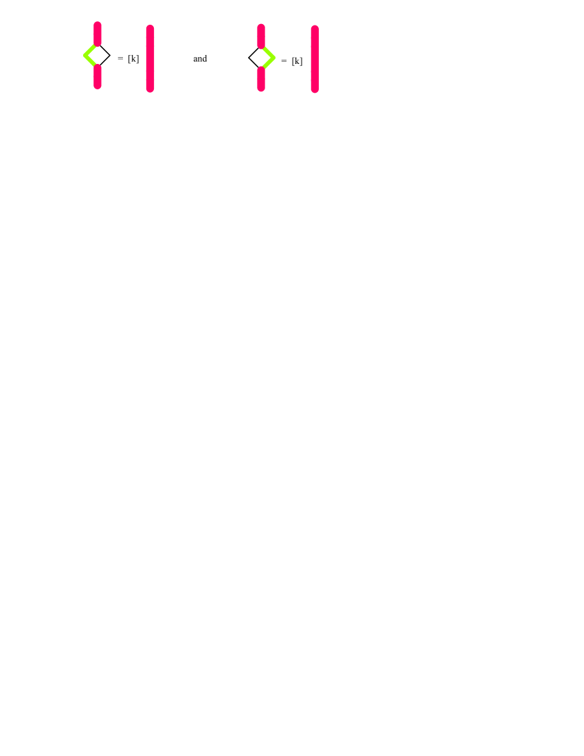
Figure 1. Relations (I): Two pairs of Intertwiners $\wedge^{k}V\rightarrow\wedge^{k}V$.

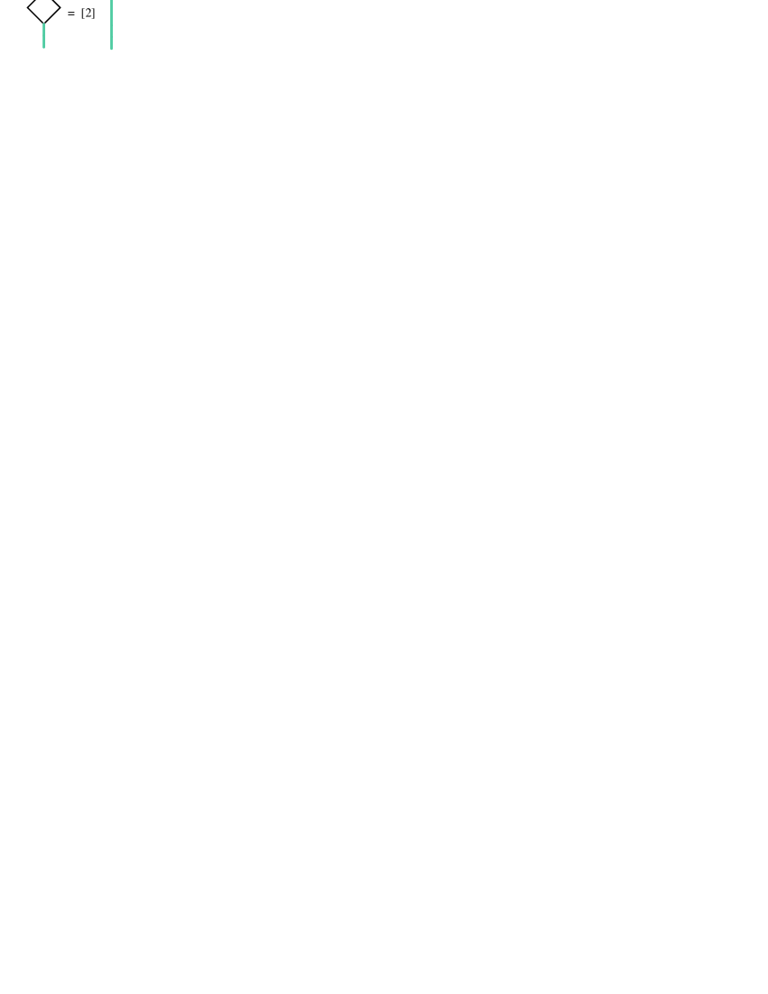
Figure 2. Relation (II): Intertwiners $\wedge^{2}V\rightarrow\wedge^{2}V$

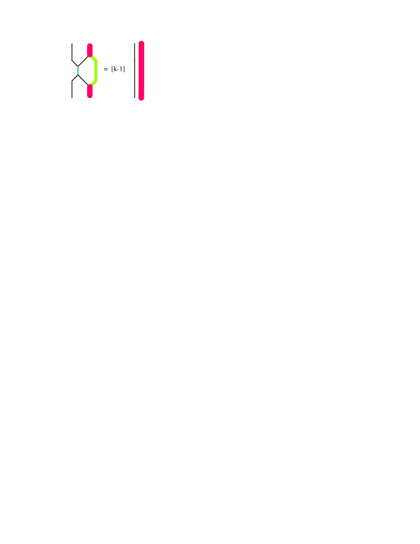
Figure 3. Relation (III): Intertwiners $V\otimes\wedge^{k}V\rightarrow V\otimes\wedge^{k}V$.

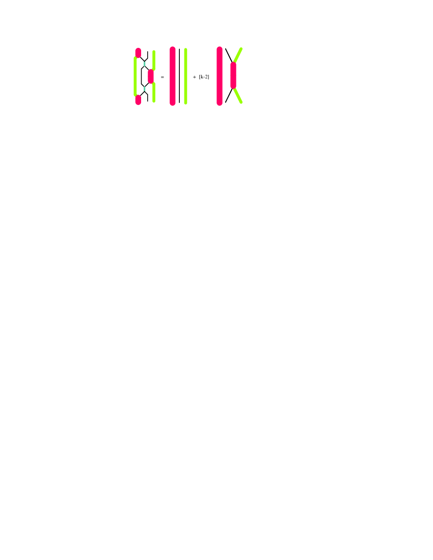
Figure 4. Relation (IV): Intertwiners $\wedge^{k}V\otimes V\otimes\wedge^{k-1}V\rightarrow\wedge^{k}V\otimes V\otimes\wedge^{k-1}V$.

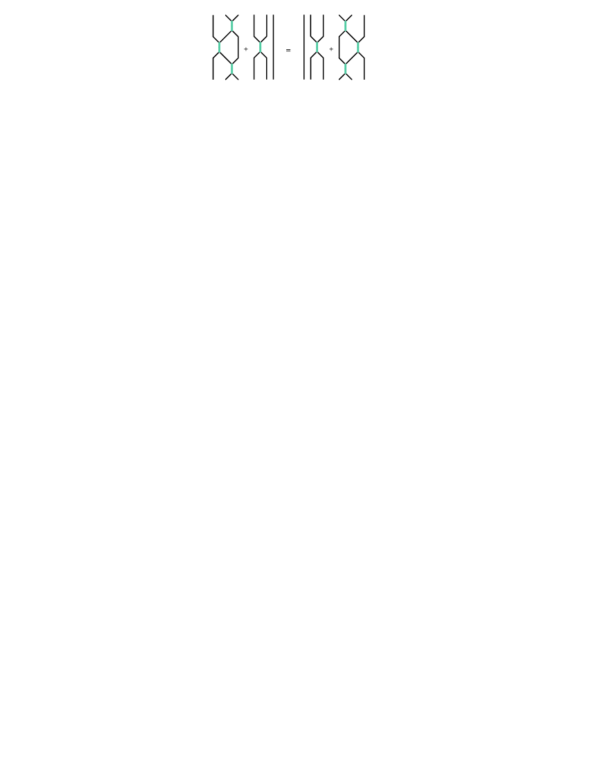
Figure 5. Relation (V): Intertwiners $V\otimes V\otimes V\rightarrow V\otimes V\otimes V$.

3. Box diagrams and fillings

Fix a positive integers $n$. Any tensor product $V^{\otimes i}$, exterior product $\wedge^{i}V$, or combination of both, comes along with the standard basis given by tensors of basis vectors of $V$ and exterior products $v_{i_{1}}\wedge v_{i_{2}}\wedge\ldots\wedge v_{i_{k}}$ with strictly decreasing indices $i_{1}>i_{2}>\ldots>i_{k}$.

A tuple $\mu=(\mu_{1},\mu_{2},\ldots,\mu_{l})$ of nonnegative integers with $\sum_{i=1}^{l}\mu_{i}=n$ is a composition of $n$, denoted $\mu\vDash n$. We call the number $l$ the length ${l}(\mu)$ of $\mu$, and the number of non-zero entries of $\mu$ the actual length, denoted ${ll}(\mu)$, of $\mu$. Associated with any composition $\mu$ we have the box diagram $D^{\mu}$ - drawn in the $\{(x,y)\mid x\geq 0,y\leq 0\}$-quadrant of the plane, numbering rows $1,2,\ldots$ from top to bottom and columns $1,2,\ldots$ from left to right - with $\mu_{i}$ boxes in the $i$th-column, placed in the rows $1$ to $\mu_{i}$ - see Examples below.

Given a box diagram $D^{\mu}$ of type $\mu$ and a second composition $\nu$ of $n$, a filling of $D^{\mu}$ of type $\nu$ is a filling of $D^{\mu}$ such that for $1\leq i\leq l(\nu)$, the number $i$ appears exactly $\nu_{i}$ times. The filling is column strict if in each column the numbers are strictly increasing from top to bottom. If $l(\mu)\leq k$ we associate to a given column strict filling $F$ of type $\nu$ of $D^{\mu}$ a standard basis element

$$\Phi(F)\in\bigwedge^{\nu}V:=\bigwedge^{\nu_{1}}{V}\otimes\bigwedge^{\nu_{2}}{V}\otimes\ldots\otimes\bigwedge^{\nu_{k}}{V}$$

as follows: Let $c_{i,1}<c_{i,2}<\ldots<c_{i,\nu_{i}}$ be the numbers of the columns, where the entry $i$ occurs, then

(3.1) $$\Phi(F):=w_{1}\otimes w_{2}\otimes\ldots\otimes w_{k}$$

where $w_{i}:=v_{c_{i,1}}\wedge v_{c_{i,2}}\wedge\ldots\wedge v_{c_{i,\nu_{i}}}$.

Examples 3.1.

Let $n=6$, $k=3$, $\nu=(2,3,1)$. Then $\bigwedge^{\nu}V$ has dimension $9$. For $\mu$ equal to $(3,2,1)$, $(3,1,2)$, $(2,1,3)$, $(2,3,1)$, $(1,2,3)$, $(1,3,2)$ there is only one possible column strict filling of type $\nu$ giving rise to the following basis vectors

$$(3,2,1) \rightsquigarrow v_{1}\wedge v_{2}\otimes v_{1}\wedge v_{2}\wedge v_{3}\otimes v_{1}$$

$$(3,1,2) \rightsquigarrow v_{1}\wedge v_{3}\otimes v_{1}\wedge v_{2}\wedge v_{3}\otimes v_{3}$$

$$(2,1,3) \rightsquigarrow v_{2}\wedge v_{3}\otimes v_{1}\wedge v_{2}\wedge v_{3}\otimes v_{3}$$

$$(2,3,1) \rightsquigarrow v_{1}\wedge v_{3}\otimes v_{1}\wedge v_{2}\wedge v_{3}\otimes v_{1},$$

$$(1,2,3) \rightsquigarrow v_{1}\wedge v_{2}\otimes v_{1}\wedge v_{2}\wedge v_{3}\otimes v_{2},$$

$$(1,3,2) \rightsquigarrow v_{2}\wedge v_{3}\otimes v_{1}\wedge v_{2}\wedge v_{3}\otimes v_{2}.$$

For $\mu=(2,2,2)$ there are the following three possible column strict fillings with corresponding basis vectors

$$\begin{array}[]{cccc}\hbox{}\vbox{\vbox{\offinterlineskip \vbox{ \hrule height=0.3pt\hbox{\vrule height=7.87202pt,width=0.3pt,depth=1.96796pt\hbox to9.84pt{\hfil$2$\hfil}\vrule height=7.87202pt,width=0.3pt,depth=1.96796pt} \hrule height=0.3pt}\vspace{-\y@linethick} \vbox{ \hrule height=0.3pt\hbox{\vrule height=7.87202pt,width=0.3pt,depth=1.96796pt\hbox to9.84pt{\hfil$3$\hfil}\vrule height=7.87202pt,width=0.3pt,depth=1.96796pt} \hrule height=0.3pt}\vspace{-\y@linethick} }}\hbox{}\vbox{\vbox{\offinterlineskip \vbox{ \hrule height=0.3pt\hbox{\vrule height=7.87202pt,width=0.3pt,depth=1.96796pt\hbox to9.84pt{\hfil$1$\hfil}\vrule height=7.87202pt,width=0.3pt,depth=1.96796pt} \hrule height=0.3pt}\vspace{-\y@linethick} \vbox{ \hrule height=0.3pt\hbox{\vrule height=7.87202pt,width=0.3pt,depth=1.96796pt\hbox to9.84pt{\hfil$2$\hfil}\vrule height=7.87202pt,width=0.3pt,depth=1.96796pt} \hrule height=0.3pt}\vspace{-\y@linethick} }}\hbox{}\vbox{\vbox{\offinterlineskip \vbox{ \hrule height=0.3pt\hbox{\vrule height=7.87202pt,width=0.3pt,depth=1.96796pt\hbox to9.84pt{\hfil$1$\hfil}\vrule height=7.87202pt,width=0.3pt,depth=1.96796pt} \hrule height=0.3pt}\vspace{-\y@linethick} \vbox{ \hrule height=0.3pt\hbox{\vrule height=7.87202pt,width=0.3pt,depth=1.96796pt\hbox to9.84pt{\hfil$2$\hfil}\vrule height=7.87202pt,width=0.3pt,depth=1.96796pt} \hrule height=0.3pt}\vspace{-\y@linethick} }}&\hbox{}\vbox{\vbox{\offinterlineskip \vbox{ \hrule height=0.3pt\hbox{\vrule height=7.87202pt,width=0.3pt,depth=1.96796pt\hbox to9.84pt{\hfil$1$\hfil}\vrule height=7.87202pt,width=0.3pt,depth=1.96796pt} \hrule height=0.3pt}\vspace{-\y@linethick} \vbox{ \hrule height=0.3pt\hbox{\vrule height=7.87202pt,width=0.3pt,depth=1.96796pt\hbox to9.84pt{\hfil$2$\hfil}\vrule height=7.87202pt,width=0.3pt,depth=1.96796pt} \hrule height=0.3pt}\vspace{-\y@linethick} }}\hbox{}\vbox{\vbox{\offinterlineskip \vbox{ \hrule height=0.3pt\hbox{\vrule height=7.87202pt,width=0.3pt,depth=1.96796pt\hbox to9.84pt{\hfil$2$\hfil}\vrule height=7.87202pt,width=0.3pt,depth=1.96796pt} \hrule height=0.3pt}\vspace{-\y@linethick} \vbox{ \hrule height=0.3pt\hbox{\vrule height=7.87202pt,width=0.3pt,depth=1.96796pt\hbox to9.84pt{\hfil$3$\hfil}\vrule height=7.87202pt,width=0.3pt,depth=1.96796pt} \hrule height=0.3pt}\vspace{-\y@linethick} }}\hbox{}\vbox{\vbox{\offinterlineskip \vbox{ \hrule height=0.3pt\hbox{\vrule height=7.87202pt,width=0.3pt,depth=1.96796pt\hbox to9.84pt{\hfil$1$\hfil}\vrule height=7.87202pt,width=0.3pt,depth=1.96796pt} \hrule height=0.3pt}\vspace{-\y@linethick} \vbox{ \hrule height=0.3pt\hbox{\vrule height=7.87202pt,width=0.3pt,depth=1.96796pt\hbox to9.84pt{\hfil$2$\hfil}\vrule height=7.87202pt,width=0.3pt,depth=1.96796pt} \hrule height=0.3pt}\vspace{-\y@linethick} }}&\hbox{}\vbox{\vbox{\offinterlineskip \vbox{ \hrule height=0.3pt\hbox{\vrule height=7.87202pt,width=0.3pt,depth=1.96796pt\hbox to9.84pt{\hfil$1$\hfil}\vrule height=7.87202pt,width=0.3pt,depth=1.96796pt} \hrule height=0.3pt}\vspace{-\y@linethick} \vbox{ \hrule height=0.3pt\hbox{\vrule height=7.87202pt,width=0.3pt,depth=1.96796pt\hbox to9.84pt{\hfil$2$\hfil}\vrule height=7.87202pt,width=0.3pt,depth=1.96796pt} \hrule height=0.3pt}\vspace{-\y@linethick} }}\hbox{}\vbox{\vbox{\offinterlineskip \vbox{ \hrule height=0.3pt\hbox{\vrule height=7.87202pt,width=0.3pt,depth=1.96796pt\hbox to9.84pt{\hfil$1$\hfil}\vrule height=7.87202pt,width=0.3pt,depth=1.96796pt} \hrule height=0.3pt}\vspace{-\y@linethick} \vbox{ \hrule height=0.3pt\hbox{\vrule height=7.87202pt,width=0.3pt,depth=1.96796pt\hbox to9.84pt{\hfil$2$\hfil}\vrule height=7.87202pt,width=0.3pt,depth=1.96796pt} \hrule height=0.3pt}\vspace{-\y@linethick} }}\hbox{}\vbox{\vbox{\offinterlineskip \vbox{ \hrule height=0.3pt\hbox{\vrule height=7.87202pt,width=0.3pt,depth=1.96796pt\hbox to9.84pt{\hfil$2$\hfil}\vrule height=7.87202pt,width=0.3pt,depth=1.96796pt} \hrule height=0.3pt}\vspace{-\y@linethick} \vbox{ \hrule height=0.3pt\hbox{\vrule height=7.87202pt,width=0.3pt,depth=1.96796pt\hbox to9.84pt{\hfil$3$\hfil}\vrule height=7.87202pt,width=0.3pt,depth=1.96796pt} \hrule height=0.3pt}\vspace{-\y@linethick} }}\\ v_{2}\wedge v_{3}\otimes v_{1}\wedge v_{2}\wedge v_{3}\otimes v_{1}&v_{1}\wedge v_{3}\otimes v_{1}\wedge v_{2}\wedge v_{3}\otimes v_{2}&v_{1}\wedge v_{2}\otimes v_{1}\wedge v_{2}\wedge v_{3}\otimes v_{3}.\end{array}$$

Let $n=2$, $k=3$, $\nu=(1,1)$, hence $\bigwedge^{\nu}V=V\otimes V$. Then we have for instance the following box diagrams, where the dots are indicating the columns with no boxes:

$$D^{(2,0,0)}=\parbox[th]{14.22636pt}{\hbox{}{\vbox{\offinterlineskip\vbox{\hrule height=0.3pt\hbox{\vrule height=8.74669pt,width=0.3pt,depth=2.18663pt\hbox to10.93333pt{\hfil}\vrule height=8.74669pt,width=0.3pt,depth=2.18663pt} \hrule height=0.3pt}\vspace{-\y@linethick} \vbox{\hrule height=0.3pt\hbox{\vrule height=8.74669pt,width=0.3pt,depth=2.18663pt\hbox to10.93333pt{\hfil}\vrule height=8.74669pt,width=0.3pt,depth=2.18663pt} \hrule height=0.3pt}\vspace{-\y@linethick} }}}\bullet\;\bullet\quad\quad\quad D^{(0,2,0)}=\bullet\;\;\parbox[th]{14.22636pt}{\hbox{}{\vbox{\offinterlineskip\vbox{\hrule height=0.3pt\hbox{\vrule height=8.74669pt,width=0.3pt,depth=2.18663pt\hbox to10.93333pt{\hfil}\vrule height=8.74669pt,width=0.3pt,depth=2.18663pt} \hrule height=0.3pt}\vspace{-\y@linethick} \vbox{\hrule height=0.3pt\hbox{\vrule height=8.74669pt,width=0.3pt,depth=2.18663pt\hbox to10.93333pt{\hfil}\vrule height=8.74669pt,width=0.3pt,depth=2.18663pt} \hrule height=0.3pt}\vspace{-\y@linethick} }}}\bullet\quad\quad\quad D^{(0,2,0)}=\bullet\;\bullet\hbox{}\vbox{\vbox{\offinterlineskip\vbox{\hrule height=0.3pt\hbox{\vrule height=8.74669pt,width=0.3pt,depth=2.18663pt\hbox to10.93333pt{\hfil}\vrule height=8.74669pt,width=0.3pt,depth=2.18663pt} \hrule height=0.3pt}\vspace{-\y@linethick} \vbox{\hrule height=0.3pt\hbox{\vrule height=8.74669pt,width=0.3pt,depth=2.18663pt\hbox to10.93333pt{\hfil}\vrule height=8.74669pt,width=0.3pt,depth=2.18663pt} \hrule height=0.3pt}\vspace{-\y@linethick} }}$$

In each case there is only one possible column strict filling of type $\nu=(1,1)$, namely    $1$        $2$     . The corresponding basis elements of $V\otimes V$ are then $v_{1}\otimes v_{1}$, $v_{2}\otimes v_{2}$ and $v_{3}\otimes v_{3}$ respectively. Figuring out the remaining basis vectors is left to the reader.

3.1. Actions of the symmetric group

Let $\hat{\mathbf{D}}^{\mu}_{\nu}$ (resp. ${\mathbf{D}}^{\mu}_{\nu}$) be the set of box diagrams of type $\mu$ with fillings (resp. column strict filling) of type $\nu$. If $\nu=(1^{n}):=(1,1,\ldots 1)$ we will normally omit the index $\nu$ in the notation. There is a special element $T^{\mu}\in{\mathbf{D}}^{\mu}$ with the standard filling given by putting the numbers $1,2,3,\dots,n$ in this order column by column from the top to the bottom; for instance

$$T^{(2,2,2)}=\parbox[th]{142.26378pt}{\hbox{}{\vbox{\offinterlineskip \vbox{ \hrule height=0.3pt\hbox{\vrule height=8.74669pt,width=0.3pt,depth=2.18663pt\hbox to10.93333pt{\hfil$1$\hfil}\vrule height=8.74669pt,width=0.3pt,depth=2.18663pt} \hrule height=0.3pt}\vspace{-\y@linethick} \vbox{ \hrule height=0.3pt\hbox{\vrule height=8.74669pt,width=0.3pt,depth=2.18663pt\hbox to10.93333pt{\hfil$2$\hfil}\vrule height=8.74669pt,width=0.3pt,depth=2.18663pt} \hrule height=0.3pt}\vspace{-\y@linethick} }}\hbox{}{\vbox{\offinterlineskip \vbox{ \hrule height=0.3pt\hbox{\vrule height=8.74669pt,width=0.3pt,depth=2.18663pt\hbox to10.93333pt{\hfil$3$\hfil}\vrule height=8.74669pt,width=0.3pt,depth=2.18663pt} \hrule height=0.3pt}\vspace{-\y@linethick} \vbox{ \hrule height=0.3pt\hbox{\vrule height=8.74669pt,width=0.3pt,depth=2.18663pt\hbox to10.93333pt{\hfil$4$\hfil}\vrule height=8.74669pt,width=0.3pt,depth=2.18663pt} \hrule height=0.3pt}\vspace{-\y@linethick} }}\hbox{}{\vbox{\offinterlineskip \vbox{ \hrule height=0.3pt\hbox{\vrule height=8.74669pt,width=0.3pt,depth=2.18663pt\hbox to10.93333pt{\hfil$5$\hfil}\vrule height=8.74669pt,width=0.3pt,depth=2.18663pt} \hrule height=0.3pt}\vspace{-\y@linethick} \vbox{ \hrule height=0.3pt\hbox{\vrule height=8.74669pt,width=0.3pt,depth=2.18663pt\hbox to10.93333pt{\hfil$6$\hfil}\vrule height=8.74669pt,width=0.3pt,depth=2.18663pt} \hrule height=0.3pt}\vspace{-\y@linethick} }}}.$$

The $i$-th box of $D^{\mu}$ is the box with the number $i$ in the standard filling; it is denoted by $b_{i}(D^{\mu})$. Let $S_{n}$ be the symmetric group with the usual generators $s_{i}$, $1\leq i\leq n-1$. Then $S_{n}$ acts on $\hat{\mathbf{D}}^{\mu}_{\nu}$ from the right by permuting the entries and from the left by permuting the boxes (with their entries).

Examples 3.2.

$T^{(2,2,2)}s_{4}s_{3}s_{2}=\hbox{}\vbox{\vbox{\offinterlineskip \vbox{ \hrule height=0.3pt\hbox{\vrule height=8.74669pt,width=0.3pt,depth=2.18663pt\hbox to10.93333pt{\hfil$1$\hfil}\vrule height=8.74669pt,width=0.3pt,depth=2.18663pt} \hrule height=0.3pt}\vspace{-\y@linethick} \vbox{ \hrule height=0.3pt\hbox{\vrule height=8.74669pt,width=0.3pt,depth=2.18663pt\hbox to10.93333pt{\hfil$3$\hfil}\vrule height=8.74669pt,width=0.3pt,depth=2.18663pt} \hrule height=0.3pt}\vspace{-\y@linethick} }}\hbox{}\vbox{\vbox{\offinterlineskip \vbox{ \hrule height=0.3pt\hbox{\vrule height=8.74669pt,width=0.3pt,depth=2.18663pt\hbox to10.93333pt{\hfil$4$\hfil}\vrule height=8.74669pt,width=0.3pt,depth=2.18663pt} \hrule height=0.3pt}\vspace{-\y@linethick} \vbox{ \hrule height=0.3pt\hbox{\vrule height=8.74669pt,width=0.3pt,depth=2.18663pt\hbox to10.93333pt{\hfil$5$\hfil}\vrule height=8.74669pt,width=0.3pt,depth=2.18663pt} \hrule height=0.3pt}\vspace{-\y@linethick} }}\hbox{}\vbox{\vbox{\offinterlineskip \vbox{ \hrule height=0.3pt\hbox{\vrule height=8.74669pt,width=0.3pt,depth=2.18663pt\hbox to10.93333pt{\hfil$2$\hfil}\vrule height=8.74669pt,width=0.3pt,depth=2.18663pt} \hrule height=0.3pt}\vspace{-\y@linethick} \vbox{ \hrule height=0.3pt\hbox{\vrule height=8.74669pt,width=0.3pt,depth=2.18663pt\hbox to10.93333pt{\hfil$6$\hfil}\vrule height=8.74669pt,width=0.3pt,depth=2.18663pt} \hrule height=0.3pt}\vspace{-\y@linethick} }}$, whereas $s_{2}s_{3}s_{4}T^{(2,2,2)}=\hbox{}\vbox{\vbox{\offinterlineskip \vbox{ \hrule height=0.3pt\hbox{\vrule height=8.74669pt,width=0.3pt,depth=2.18663pt\hbox to10.93333pt{\hfil$1$\hfil}\vrule height=8.74669pt,width=0.3pt,depth=2.18663pt} \hrule height=0.3pt}\vspace{-\y@linethick} \vbox{ \hrule height=0.3pt\hbox{\vrule height=8.74669pt,width=0.3pt,depth=2.18663pt\hbox to10.93333pt{\hfil$5$\hfil}\vrule height=8.74669pt,width=0.3pt,depth=2.18663pt} \hrule height=0.3pt}\vspace{-\y@linethick} }}\hbox{}\vbox{\vbox{\offinterlineskip \vbox{ \hrule height=0.3pt\hbox{\vrule height=8.74669pt,width=0.3pt,depth=2.18663pt\hbox to10.93333pt{\hfil$2$\hfil}\vrule height=8.74669pt,width=0.3pt,depth=2.18663pt} \hrule height=0.3pt}\vspace{-\y@linethick} \vbox{ \hrule height=0.3pt\hbox{\vrule height=8.74669pt,width=0.3pt,depth=2.18663pt\hbox to10.93333pt{\hfil$3$\hfil}\vrule height=8.74669pt,width=0.3pt,depth=2.18663pt} \hrule height=0.3pt}\vspace{-\y@linethick} }}\hbox{}\vbox{\vbox{\offinterlineskip \vbox{ \hrule height=0.3pt\hbox{\vrule height=8.74669pt,width=0.3pt,depth=2.18663pt\hbox to10.93333pt{\hfil$4$\hfil}\vrule height=8.74669pt,width=0.3pt,depth=2.18663pt} \hrule height=0.3pt}\vspace{-\y@linethick} \vbox{ \hrule height=0.3pt\hbox{\vrule height=8.74669pt,width=0.3pt,depth=2.18663pt\hbox to10.93333pt{\hfil$6$\hfil}\vrule height=8.74669pt,width=0.3pt,depth=2.18663pt} \hrule height=0.3pt}\vspace{-\y@linethick} }}$.

3.2. The correspondence

For any composition $\mu$ of $n$ let $\tilde{\mu}$ be the reduced composition obtained by disregarding the zero entries of $\mu$. Let $S_{\mu}$ be the corresponding Young subgroup, i.e. $S_{\mu}=S_{\tilde{\mu}_{1}}\times S_{\tilde{\mu}_{2}}\times S_{\tilde{\mu}_{ll(\mu)}}$ of $S_{n}$. We denote by ${}^{\mu}S_{n}$ the set of shortest coset representatives in $S_{\mu}\backslash S_{n}$, similarly let $S_{n}^{\mu}$ be the set of shortest coset representatives in $S_{n}/S_{\mu}$. Let $\bf{O}^{\mu}_{\nu}$ denote the set of cosets $c\in S_{n}/S_{\nu}$ such that $w\in{}^{\mu}S_{n}$ for any $w\in c$.

Assume we have a box diagram $D$ and $\nu\vDash n$. Then any filling of type $\nu$ can be transferred into a filling of type $(1^{n})$ by replacing first all ones by the numbers $1,2,\ldots,\nu_{i}$ from left to right, then all two’s by the numbers $\nu_{1}+1,\ldots\nu_{1}+\nu_{2}$ etc. On the other hand, if we have a filling $F$ of type $(1^{n})$ then we can replace the first $\nu_{1}$ numbers by $1$’s, the next $\nu_{2}$ numbers by $2$’s etc. We call the result $\psi_{\nu}(F)$. The latter is always an element of $\hat{{\mathbf{D}}}^{\mu}_{\nu}$, but not necessarily of ${\mathbf{D}}^{\mu}_{\nu}$. We have however the following result

Lemma 3.3.

1. Let $\mu\vDash n$ and $w\in S_{n}$, then $wT^{\mu}=T^{\mu}w$.

2. The map $\Phi$ from (3.1) defines a bijection

   $$\Phi_{\nu}^{\mu}:\quad\bigcup_{l(\mu)\leq k}{\mathbf{D}}^{\mu}_{\nu} \stackrel{{\scriptstyle 1:1}}{{\leftrightarrow}} \text{ elements of the standard basis of }\bigwedge^{\nu}{V}$$

3. There is a bijection

   $$\Psi_{\nu}^{\mu}:\quad\bf{O}^{\mu}_{\nu} \stackrel{{\scriptstyle 1:1}}{{\leftrightarrow}} {\mathbf{D}}^{\mu}_{\nu}$$

   $$w \mapsto \psi_{\nu}(wT^{\mu}).$$

Proof.

By definition, the entry of the $i$th-box of $T^{\mu}$ is precisely $i$, so the first statement is obvious. The map $\Phi_{\nu}^{\mu}$ is obviously injective. To see that it is surjective note that a basis of $\bigwedge^{\nu}V$ is given by elements of the form $w_{1}\otimes w_{2}\otimes\ldots\otimes w_{k}$ where $w_{i}:=v_{c_{i,1}}\wedge v_{c_{i,2}}\wedge\ldots\wedge v_{c_{i,r_{i}}}$, where for any $i$ we have $c_{i,1}<{c_{i,2}}<\ldots<{c_{i,r_{i}}}$ and $1\leq c_{i,j}\leq k$. A preimage of $w_{1}\otimes w_{2}\otimes\ldots\otimes w_{k}$ can be constructed as follows: we create a box diagram with column strict filling by putting ones in the columns $c_{(1,j)}$, then $2$’s in the columns $c_{(2,j)}$ etc. As a result we get an element in $\bigcup_{l(\mu)\leq k}{\mathbf{D}}^{\mu}_{\nu}$ which is obviously a preimage, and $\Phi_{\nu}^{\mu}$ is surjective.

Let’s take the box diagram $T^{\mu}$ associated with $\mu$ with the standard filling. $S_{n}$ acts transitively from the left on $\hat{\mathbf{D}}^{\mu}$ giving rise to a bijection $\alpha:S_{n}\cong S_{n}T^{\mu}$. From the definition of the left action of $S_{n}$ on diagrams with fillings we get directly that $wT^{\mu}\in{}^{\mu}S_{n}$ if and only if, in each column, the entries are strictly increasing from top to bottom. Hence $\Psi_{\nu}^{\mu}$ is a bijection if $\nu=(1^{n})$. If $\nu$ is now arbitrary, then $w\in\bf{O}^{\mu}_{\nu}$ if and only if the entries in the columns are still strictly increasing from top to bottom if we replace the first $\nu_{1}$ numbers by ones, then the next $\nu_{2}$ numbers by twos etc. The claim is then obvious. ∎

For any set $M$ let $\mathbb{C}[M]$ be the free $\mathbb{C}$-module with basis given by the elements of $M$. If $\mu=1^{n}$, then the action of $S_{n}$ turns $\mathbb{C}[{\mathbf{D}}^{\mu}]$ into the permutation module, which is a special instance of the induced sign module $N(\mu)=\mathbb{C}[S_{n}]\otimes_{\mathbb{C}[S_{\mu}]}\operatorname{sgn}$ for arbitrary $\mu$. The latter has a basis given by $x\otimes 1$, $x\in{}^{\mu}S_{n}$. We identify this space in the obvious way with $\mathbb{C}[\bf{O}^{\mu}]$ and $\mathbb{C}[{\mathbf{D}}^{\mu}]$ so that Lemma 3.3 induces isomorphisms of $S_{n}$-modules $\mathbb{C}[\bf{O}^{\mu}]\cong\mathbb{C}[{\mathbf{D}}^{\mu}]$ and $\bigoplus_{\mu}\mathbb{C}[{\mathbf{D}}^{\mu}]\cong{V}^{\otimes n}$ where $S_{n}$ acts by permuting the factors.

All this can be quantised: If ${}^{\mathbb{Z}}\bf{O}^{\mu}_{\nu}$ denotes the free $\mathbb{C}[q,q^{-1}]$-module with basis $\bf{O}^{\mu}_{\nu}$ then we view ${}^{\mathbb{Z}}\bf{O}^{\mu}$ as the induced sign module ${\mathcal{N}}(\mu)=H_{q}(S_{n})\otimes_{H_{q}(S_{\mu})}\operatorname{sgn}$ for the Iwahori-Hecke algebra $H_{q}(S_{n})$ and

$$\bigoplus_{\mu}{}^{\mathbb{Z}}{\bf O}^{\mu}\cong V^{\otimes n}$$

where $H_{q}(S_{n})$ acts via the $R$-matrix.

The Hecke algebra $H_{q}(S_{n})$ comes along with the standard basis $H_{x}$, $x\in S_{n}$, and with the Kazhdan-Lusztig basis $\underline{H}_{x}$, $x\in S_{n}$. In the following we use the normalisation of [26]. In particular, $\underline{H}_{s}=H_{s}+qH_{e}=:H_{s}+q$. Associated with $x\in S_{n}$ we have $(t(x),t^{\prime}(x))$, the corresponding pair of standard tableaux via the Robinson-Schensted correspondence. We will need the following well-known result (see e.g. [12, Section3]): If $t(x)$ has more than $ll(\mu)$ rows then $\underline{H}_{x}$ is in the annihilator of ${}^{\mathbb{Z}}\bf{O}^{\mu}$.

3.3. Category ${\mathcal{O}}$

We consider the Lie algebra $\mathfrak{gl}_{n}$ and the corresponding Bernstein-Gelfand-Gelfand category ${\mathcal{O}}={\mathcal{O}}(n)$ associated with the standard triangular decomposition $\mathfrak{gl}_{n}=\mathfrak{n}_{-}\oplus\mathfrak{\mathfrak{h}}\oplus\mathfrak{\mathfrak{n}}=\mathfrak{n}_{-}\oplus\mathfrak{b}$, see [3]. The Weyl group is identified with the permutation group $S_{n}$ in the standard way.

For any composition $\lambda$ of $n$ we fix an integral block ${\mathcal{O}}_{\tilde{\lambda}}$ of ${\mathcal{O}}$ such that the projective Verma module in this block has highest weight $\tilde{\lambda}$, and the stabiliser of $\tilde{\lambda}$ is $S_{\lambda}$. By abuse of notation we denote this block by ${\mathcal{O}}_{\lambda}$ and the highest weight of the projective Verma module $P(\tilde{\lambda})=M(\tilde{\lambda})\in{\mathcal{O}}_{\tilde{\lambda}}$ by $\lambda$. For $\mu\vDash n$ let ${\mathcal{O}}^{\mu}_{\lambda}$ be the subcategory given by all locally $\mathfrak{p}$-finite objects, where $\mathfrak{p}$ is the parabolic (containing $\mathfrak{b}$) with Weyl group $S_{\mu}$. The simple objects in ${\mathcal{O}}_{\lambda}$ are exactly the simple highest weight modules $L(x\cdot\lambda)$ with $x\in S_{n}^{\lambda}$, with the corresponding Verma modules $M(x\cdot\lambda)$. The simple objects in ${\mathcal{O}}_{\lambda}^{\mu}$ are exactly the simple highest weight modules $L(x\cdot\lambda)$ with $x\in\bf{O}_{\lambda}^{\mu}$. In particular, $\mathbb{C}[\bf{O}_{\lambda}^{\mu}]$ can be identified with the complexified Grothendieck group of ${\mathcal{O}}_{\lambda}^{\mu}$ by mapping $x\in\bf{O}_{\lambda}^{\mu}$ to the isomorphism class of the parabolic Verma module $M^{\mu}(x\cdot\lambda)$ with highest weight $x\cdot\lambda$.

We denote by ${}^{\mathbb{Z}}{\mathcal{O}}_{\lambda}^{\mu}$ the graded version of ${\mathcal{O}}_{\lambda}^{\mu}$ as introduced in [2] and further developed in [27] and [28, Section 2]. Each parabolic Verma module $M^{\mu}(x\cdot\lambda)\in{\mathcal{O}}_{\lambda}^{\mu}$ has a standard graded lift $\Delta(x\cdot\lambda)\in{}^{\mathbb{Z}}{\mathcal{O}}_{\lambda}^{\mu}$ with head concentrated in degree zero. For $j\in\mathbb{Z}$ we denote by $\Delta(x\cdot\lambda)\langle j\rangle$ the lift with head in degree $j$, in particular $\Delta(x\cdot\lambda)\langle 0\rangle=\Delta(x\cdot\lambda)$. Let $P(x\cdot\lambda)\langle j\rangle$ be the indecomposable projective cover of $\Delta(x\cdot\lambda)\langle j\rangle$. More generally, we denote by $\langle j\rangle$ the functor which shifts the grading up by $j\in\mathbb{Z}$.

Note that the complexified Grothendieck group $[^{\mathbb{Z}}{\mathcal{O}}_{\lambda}^{\mu}]$ of ${}^{\mathbb{Z}}{\mathcal{O}}_{\lambda}^{\mu}$ is naturally isomorphic to ${}^{\mathbb{Z}}\bf{O}_{\lambda}^{\mu}$ by mapping $\Delta(x\cdot\lambda)\langle j\rangle$ to $q^{j}x$. In the following we will abuse notation and denote $\Delta(x\cdot\lambda)\langle j\rangle$ by $q^{j}\Delta(x\cdot\lambda)$ or even by $q^{j}\Delta(x)$ or $q^{j}\Delta(i_{1}\;i_{2}\ldots i_{r})$ if $x=s_{i_{1}}\ldots s_{i_{r}}$ is a reduced expression for $x$ and it is clear from the context to which category the module belongs to. Analogous abbreviations will be used for the projectives $P(x\cdot\lambda)\langle j\rangle$.

4. The same combinatorics in three disguises

4.1. Translation functors - combinatorially

We first recall the explicit combinatorics of special projective functors, namely the translation functors on and out of the walls. Thanks to Fact 1 below the combinatorics describes the functor completely.

Let $\lambda,\mu\vDash n$. If $S_{\lambda}\subseteq S_{\nu}$ then there is the translation out of the walls functor (see [13, 4.11])

$$T_{\nu}^{\lambda}:\;{\mathcal{O}}(n)_{\nu}\longrightarrow{\mathcal{O}}(n)_{\lambda}$$

with its standard graded lift

$$\theta_{\nu}^{\lambda}:\;{}^{\mathbb{Z}}{\mathcal{O}}(n)_{\nu}\longrightarrow{}^{\mathbb{Z}}{\mathcal{O}}(n)_{\lambda}$$

which is uniquely determined by requiring that $\Delta(e)$ is mapped to a standard lift of the (indecomposable) projective module $T_{\nu}^{\lambda}M(\nu)$. In the following we will only need special instances of translation functors (analogous to our special choices of intertwiners in Section 2.1). Let $\nu,\lambda\vDash n$ such that there exists some $l$ such that $\lambda_{t}=\nu_{t}$ for $t<l$, $\lambda_{t+1}=\nu_{t}$ for $t>l+1$ and set $j=\lambda_{1}+...\lambda_{l-1}$.

1. If moreover $\lambda_{l}=1$, $\lambda_{l+1}=i$, $\nu_{l}=i+1$ then $\theta_{\nu}^{\lambda}:\;{}^{\mathbb{Z}}{\mathcal{O}}(n)_{\nu}\longrightarrow{}^{\mathbb{Z}}{\mathcal{O}}(n)_{\lambda}$ maps $\Delta(e)$ to the graded projective module $P((i+j)(i+j-1)\ldots(j+1))$. The latter has each of the following:

   $$\Delta((j+i)...(j+1)),\;q\Delta((j+i-1)...(j+1)),\;...,\;q^{i}\Delta(e)$$

   exactly once as graded Verma subquotients. To abbreviate this we will say $\Delta(e)$ is mapped to $A_{j+i}^{j+1}$ as defined in (5.6).

2. If moreover $\lambda_{l}=i$, $\lambda_{l+1}=1$, $\nu_{l}=i+1$, then $\theta_{\nu}^{\lambda}:\;{}^{\mathbb{Z}}{\mathcal{O}}(n)_{\nu}\longrightarrow{}^{\mathbb{Z}}{\mathcal{O}}(n)_{\lambda}$ maps $\Delta(e)$ to the graded projective $P\left((j+1)\;(j+2)\ldots(j+i)\right)$ which has

   $$\Delta\left((1+j)\ldots(i+j)\right),\;q\Delta\left((2+j)\ldots(i+j)\right),\;\ldots,$$

   $$q^{i-1}\Delta(i+j),\;q^{i}\Delta(e),$$

   as graded Verma subquotients. In a short form we say that $\Delta(e)$ is mapped to $B_{j+1}^{i+j}$ as defined in (5.6).

Translation functors preserve parabolic subcategories, hence it makes sense to define

$$\bigcurlyvee_{(i+j)}^{(i,\,\,j)} = \bigoplus_{\mu}\theta_{(i+j)}^{(i,j)}:\quad\bigoplus_{\mu}{}^{\mathbb{Z}}{\mathcal{O}}(i+j)^{\mu}_{(i+j)}\longrightarrow\bigoplus_{\mu}{}^{\mathbb{Z}}{\mathcal{O}}(i+j)^{\mu}_{(i,j)}.$$

where the sum runs over all compositions $\mu$ of length at most $k$.

Again if we have $S_{\lambda}\subseteq S_{\nu}$ there is also the translation onto the walls functor $T_{\lambda}^{\nu}:{\mathcal{O}}(n)_{\lambda}\longrightarrow{\mathcal{O}}(n)_{\nu}$. We have its standard graded lift

$$\theta_{\lambda}^{\nu}:{}^{\mathbb{Z}}{\mathcal{O}}(n)_{\lambda}\longrightarrow{}^{\mathbb{Z}}{\mathcal{O}}(n)_{\nu}$$

which maps $\Delta(x)$ to $q^{-r}\Delta(z)$, where $z$ and $r$ are defined by writing $x=zy$ with $y\in S_{\nu}$, and $z\in S_{n}^{\nu}$ a shortest coset representative and $r=l(y)$ being the length of $y$. We define

$$\bigcurlywedge^{(i+j)}_{(i,\,\,j)}=\bigoplus_{\mu}\theta_{(i,j)}^{(i+j)}:\quad\bigoplus_{\mu}{}^{\mathbb{Z}}{\mathcal{O}}(i+j)^{\mu}_{(i,j)}\longrightarrow\bigoplus_{\mu}{}^{\mathbb{Z}}{\mathcal{O}}(i+j)^{\mu}_{(i+j)},$$

where the sum runs over all compositions $\mu$ of length at most $k$.

Let $\lambda$, $\nu$, $\mu$ be compositions of $n$. Translation functors out and onto walls are special instances of projective functors. We denote by ${\mathcal{P}}(\lambda,\nu)$ the set of projective functors from ${\mathcal{O}}_{\lambda}$ to ${\mathcal{O}}_{\nu}$ as introduced and classified in [5]. We recall the following well-known facts:

1. ([5]) A projective functor $F\in{\mathcal{P}}(\lambda,\nu)$ is (up to isomorphism) completely determined by its value on $M(\lambda)$, i.e. we have an isomorphism of projective functors $F\cong G$ if and only if there is an isomorphism of modules $FM(\lambda)\cong GM(\lambda)$. More precisely: $FM(\lambda)\in{\mathcal{O}}_{\nu}$ is projective and $F$ decomposes into indecomposable summands exactly according to the decomposition of $FM(\lambda)$ into indecomposable direct summands.

2. ([28, Corollary 3.12], [27]) Let $F\in{\mathcal{P}}(\lambda,\nu)$ be indecomposable. There exists a graded lift $\tilde{F}:{}^{\mathbb{Z}}{\mathcal{O}}_{\lambda}\rightarrow{}^{\mathbb{Z}}{\mathcal{O}}_{\nu}$. Up to isomorphism and shift in the grading it is unique, and up to isomorphism completely determined by its value on $\Delta(e)\in{}^{\mathbb{Z}}{\mathcal{O}}_{\lambda}$ (thanks to Fact 1).

3. ([28, Proposition 4.2] and references therein) Let $F\in{\mathcal{P}}(\lambda,\nu)$ be indecomposable such that $\theta_{\nu}^{(1^{n})}FM(\lambda)\cong P(x)$. Assume the tableau $t(x)$ has more than $k$ rows. Then the restriction of $F$ to ${\mathcal{O}}_{\lambda}^{\mu}$ is zero for any $\mu$ with $ll(\mu)\leq k$.

4.2. The combinatorial action of trivalent graphs

We define $\mathbb{C}[q,q^{-1}]$-linear maps

$$\bigcurlywedge_{(i,\;\;j)}^{(i+j)}:\quad\bigoplus_{\mu}\mathbb{C}[{\mathbf{D}}_{(i,j)}^{\mu}] \rightarrow \bigoplus_{\mu}\mathbb{C}[{\mathbf{D}}_{(i+j)}^{\mu}]$$

$$\bigcurlyvee^{(i,\;\;j)}_{(i+j)}:\quad\bigoplus_{\mu}\mathbb{C}[{\mathbf{D}}_{(i+j)}^{\mu}] \rightarrow \bigoplus_{\mu}\mathbb{C}[{\mathbf{D}}_{(i,j)}^{\mu}]$$

where $\mu$ runs over all compositions of $i+j$ with at most $k$ parts, as follows: In the first case we write any box diagram $D$ with filling of type $(i,j)$ as $D=x\psi_{(i,j)}T^{\mu}$ with $x$ of smallest possible length. Then $D$ is mapped to a box diagram $q^{-l(x)}D^{\prime}$ where $D^{\prime}\in{\mathbf{D}}^{\mu}_{(i+j)}$ has the same shape as $D$, but for the filling we replace the $2$’s by $1$’s. In the second case a box diagram $D$ of type $\mu$ and filling $(i+j)$ is mapped to $\sum_{I}q^{l_{I}}D_{I}$, where $I$ runs through all possible subsets of cardinality $j$ of the set of boxes of $D$. The diagram $D_{I}$ is obtained from $D$ by replacing all $1$’s in the boxes from $I$ by $2$’s, and $l_{I}$ is equal to $ij$ minus the length of the element $x$ of minimal length such that $D_{I}=x\psi_{(i,j)}T^{\mu}$.

Examples 4.1.

Let $\nu=(3)$, $\nu^{\prime}=(2,1)$ and $r=1$. Then

$$\bigcurlyvee^{(2,1)}_{(3)}(\hbox{}\vbox{\vbox{\offinterlineskip \vbox{ \hrule height=0.3pt\hbox{\vrule height=7.87202pt,width=0.3pt,depth=1.96796pt\hbox to9.84pt{\hfil$1$\hfil}\vrule height=7.87202pt,width=0.3pt,depth=1.96796pt} \hrule height=0.3pt}\vspace{-\y@linethick} }}\hbox{}\vbox{\vbox{\offinterlineskip \vbox{ \hrule height=0.3pt\hbox{\vrule height=7.87202pt,width=0.3pt,depth=1.96796pt\hbox to9.84pt{\hfil$1$\hfil}\vrule height=7.87202pt,width=0.3pt,depth=1.96796pt} \hrule height=0.3pt}\vspace{-\y@linethick} }}\hbox{}\vbox{\vbox{\offinterlineskip \vbox{ \hrule height=0.3pt\hbox{\vrule height=7.87202pt,width=0.3pt,depth=1.96796pt\hbox to9.84pt{\hfil$1$\hfil}\vrule height=7.87202pt,width=0.3pt,depth=1.96796pt} \hrule height=0.3pt}\vspace{-\y@linethick} }})= \hbox{}\vbox{\vbox{\offinterlineskip \vbox{ \hrule height=0.3pt\hbox{\vrule height=7.87202pt,width=0.3pt,depth=1.96796pt\hbox to9.84pt{\hfil$2$\hfil}\vrule height=7.87202pt,width=0.3pt,depth=1.96796pt} \hrule height=0.3pt}\vspace{-\y@linethick} }}\hbox{}\vbox{\vbox{\offinterlineskip \vbox{ \hrule height=0.3pt\hbox{\vrule height=7.87202pt,width=0.3pt,depth=1.96796pt\hbox to9.84pt{\hfil$1$\hfil}\vrule height=7.87202pt,width=0.3pt,depth=1.96796pt} \hrule height=0.3pt}\vspace{-\y@linethick} }}\hbox{}\vbox{\vbox{\offinterlineskip \vbox{ \hrule height=0.3pt\hbox{\vrule height=7.87202pt,width=0.3pt,depth=1.96796pt\hbox to9.84pt{\hfil$1$\hfil}\vrule height=7.87202pt,width=0.3pt,depth=1.96796pt} \hrule height=0.3pt}\vspace{-\y@linethick} }}+q\hbox{}\vbox{\vbox{\offinterlineskip \vbox{ \hrule height=0.3pt\hbox{\vrule height=7.87202pt,width=0.3pt,depth=1.96796pt\hbox to9.84pt{\hfil$1$\hfil}\vrule height=7.87202pt,width=0.3pt,depth=1.96796pt} \hrule height=0.3pt}\vspace{-\y@linethick} }}\hbox{}\vbox{\vbox{\offinterlineskip \vbox{ \hrule height=0.3pt\hbox{\vrule height=7.87202pt,width=0.3pt,depth=1.96796pt\hbox to9.84pt{\hfil$2$\hfil}\vrule height=7.87202pt,width=0.3pt,depth=1.96796pt} \hrule height=0.3pt}\vspace{-\y@linethick} }}\hbox{}\vbox{\vbox{\offinterlineskip \vbox{ \hrule height=0.3pt\hbox{\vrule height=7.87202pt,width=0.3pt,depth=1.96796pt\hbox to9.84pt{\hfil$1$\hfil}\vrule height=7.87202pt,width=0.3pt,depth=1.96796pt} \hrule height=0.3pt}\vspace{-\y@linethick} }}+q^{2}\hbox{}\vbox{\vbox{\offinterlineskip \vbox{ \hrule height=0.3pt\hbox{\vrule height=7.87202pt,width=0.3pt,depth=1.96796pt\hbox to9.84pt{\hfil$1$\hfil}\vrule height=7.87202pt,width=0.3pt,depth=1.96796pt} \hrule height=0.3pt}\vspace{-\y@linethick} }}\hbox{}\vbox{\vbox{\offinterlineskip \vbox{ \hrule height=0.3pt\hbox{\vrule height=7.87202pt,width=0.3pt,depth=1.96796pt\hbox to9.84pt{\hfil$1$\hfil}\vrule height=7.87202pt,width=0.3pt,depth=1.96796pt} \hrule height=0.3pt}\vspace{-\y@linethick} }}\hbox{}\vbox{\vbox{\offinterlineskip \vbox{ \hrule height=0.3pt\hbox{\vrule height=7.87202pt,width=0.3pt,depth=1.96796pt\hbox to9.84pt{\hfil$2$\hfil}\vrule height=7.87202pt,width=0.3pt,depth=1.96796pt} \hrule height=0.3pt}\vspace{-\y@linethick} }}$$

$$\bigcurlywedge_{(2,1)}^{(3)}(\hbox{}\vbox{\vbox{\offinterlineskip \vbox{ \hrule height=0.3pt\hbox{\vrule height=7.87202pt,width=0.3pt,depth=1.96796pt\hbox to9.84pt{\hfil$2$\hfil}\vrule height=7.87202pt,width=0.3pt,depth=1.96796pt} \hrule height=0.3pt}\vspace{-\y@linethick} }}\hbox{}\vbox{\vbox{\offinterlineskip \vbox{ \hrule height=0.3pt\hbox{\vrule height=7.87202pt,width=0.3pt,depth=1.96796pt\hbox to9.84pt{\hfil$1$\hfil}\vrule height=7.87202pt,width=0.3pt,depth=1.96796pt} \hrule height=0.3pt}\vspace{-\y@linethick} }}\hbox{}\vbox{\vbox{\offinterlineskip \vbox{ \hrule height=0.3pt\hbox{\vrule height=7.87202pt,width=0.3pt,depth=1.96796pt\hbox to9.84pt{\hfil$1$\hfil}\vrule height=7.87202pt,width=0.3pt,depth=1.96796pt} \hrule height=0.3pt}\vspace{-\y@linethick} }})=q^{-2}\hbox{}\vbox{\vbox{\offinterlineskip \vbox{ \hrule height=0.3pt\hbox{\vrule height=7.87202pt,width=0.3pt,depth=1.96796pt\hbox to9.84pt{\hfil$1$\hfil}\vrule height=7.87202pt,width=0.3pt,depth=1.96796pt} \hrule height=0.3pt}\vspace{-\y@linethick} }}\hbox{}\vbox{\vbox{\offinterlineskip \vbox{ \hrule height=0.3pt\hbox{\vrule height=7.87202pt,width=0.3pt,depth=1.96796pt\hbox to9.84pt{\hfil$1$\hfil}\vrule height=7.87202pt,width=0.3pt,depth=1.96796pt} \hrule height=0.3pt}\vspace{-\y@linethick} }}\hbox{}\vbox{\vbox{\offinterlineskip \vbox{ \hrule height=0.3pt\hbox{\vrule height=7.87202pt,width=0.3pt,depth=1.96796pt\hbox to9.84pt{\hfil$1$\hfil}\vrule height=7.87202pt,width=0.3pt,depth=1.96796pt} \hrule height=0.3pt}\vspace{-\y@linethick} }} \displaystyle\bigcurlywedge_{(2,1)}^{(3)}(\hbox{}\vbox{\vbox{\offinterlineskip \vbox{ \hrule height=0.3pt\hbox{\vrule height=7.87202pt,width=0.3pt,depth=1.96796pt\hbox to9.84pt{\hfil$1$\hfil}\vrule height=7.87202pt,width=0.3pt,depth=1.96796pt} \hrule height=0.3pt}\vspace{-\y@linethick} }}\hbox{}\vbox{\vbox{\offinterlineskip \vbox{ \hrule height=0.3pt\hbox{\vrule height=7.87202pt,width=0.3pt,depth=1.96796pt\hbox to9.84pt{\hfil$2$\hfil}\vrule height=7.87202pt,width=0.3pt,depth=1.96796pt} \hrule height=0.3pt}\vspace{-\y@linethick} }}\hbox{}\vbox{\vbox{\offinterlineskip \vbox{ \hrule height=0.3pt\hbox{\vrule height=7.87202pt,width=0.3pt,depth=1.96796pt\hbox to9.84pt{\hfil$1$\hfil}\vrule height=7.87202pt,width=0.3pt,depth=1.96796pt} \hrule height=0.3pt}\vspace{-\y@linethick} }})=q^{-1}\hbox{}\vbox{\vbox{\offinterlineskip \vbox{ \hrule height=0.3pt\hbox{\vrule height=7.87202pt,width=0.3pt,depth=1.96796pt\hbox to9.84pt{\hfil$1$\hfil}\vrule height=7.87202pt,width=0.3pt,depth=1.96796pt} \hrule height=0.3pt}\vspace{-\y@linethick} }}\hbox{}\vbox{\vbox{\offinterlineskip \vbox{ \hrule height=0.3pt\hbox{\vrule height=7.87202pt,width=0.3pt,depth=1.96796pt\hbox to9.84pt{\hfil$1$\hfil}\vrule height=7.87202pt,width=0.3pt,depth=1.96796pt} \hrule height=0.3pt}\vspace{-\y@linethick} }}\hbox{}\vbox{\vbox{\offinterlineskip \vbox{ \hrule height=0.3pt\hbox{\vrule height=7.87202pt,width=0.3pt,depth=1.96796pt\hbox to9.84pt{\hfil$1$\hfil}\vrule height=7.87202pt,width=0.3pt,depth=1.96796pt} \hrule height=0.3pt}\vspace{-\y@linethick} }} \bigcurlywedge_{(2,1)}^{(3)}(\hbox{}\vbox{\vbox{\offinterlineskip \vbox{ \hrule height=0.3pt\hbox{\vrule height=7.87202pt,width=0.3pt,depth=1.96796pt\hbox to9.84pt{\hfil$1$\hfil}\vrule height=7.87202pt,width=0.3pt,depth=1.96796pt} \hrule height=0.3pt}\vspace{-\y@linethick} }}\hbox{}\vbox{\vbox{\offinterlineskip \vbox{ \hrule height=0.3pt\hbox{\vrule height=7.87202pt,width=0.3pt,depth=1.96796pt\hbox to9.84pt{\hfil$1$\hfil}\vrule height=7.87202pt,width=0.3pt,depth=1.96796pt} \hrule height=0.3pt}\vspace{-\y@linethick} }}\hbox{}\vbox{\vbox{\offinterlineskip \vbox{ \hrule height=0.3pt\hbox{\vrule height=7.87202pt,width=0.3pt,depth=1.96796pt\hbox to9.84pt{\hfil$2$\hfil}\vrule height=7.87202pt,width=0.3pt,depth=1.96796pt} \hrule height=0.3pt}\vspace{-\y@linethick} }})=\hbox{}\vbox{\vbox{\offinterlineskip \vbox{ \hrule height=0.3pt\hbox{\vrule height=7.87202pt,width=0.3pt,depth=1.96796pt\hbox to9.84pt{\hfil$1$\hfil}\vrule height=7.87202pt,width=0.3pt,depth=1.96796pt} \hrule height=0.3pt}\vspace{-\y@linethick} }}\hbox{}\vbox{\vbox{\offinterlineskip \vbox{ \hrule height=0.3pt\hbox{\vrule height=7.87202pt,width=0.3pt,depth=1.96796pt\hbox to9.84pt{\hfil$1$\hfil}\vrule height=7.87202pt,width=0.3pt,depth=1.96796pt} \hrule height=0.3pt}\vspace{-\y@linethick} }}\hbox{}\vbox{\vbox{\offinterlineskip \vbox{ \hrule height=0.3pt\hbox{\vrule height=7.87202pt,width=0.3pt,depth=1.96796pt\hbox to9.84pt{\hfil$1$\hfil}\vrule height=7.87202pt,width=0.3pt,depth=1.96796pt} \hrule height=0.3pt}\vspace{-\y@linethick} }}$$

We have the obvious generalisation of this procedure if $\lambda$ and $\nu$ are of the form as in (Case 1) or (Case 2), namely the role played by the entries $1$ and $2$ above is then the role of $j+1$ and $j+2$. This defines the maps $\displaystyle\bigcurlyvee^{\lambda}_{\nu}:\bigoplus_{\mu}\mathbb{C}[{\mathbf{D}}_{\nu}^{\mu}]\rightarrow\bigoplus_{\mu}\mathbb{C}[{\mathbf{D}}_{\lambda}^{\mu}]$ and $\displaystyle\bigcurlywedge_{\lambda}^{\nu}:\quad\bigoplus_{\mu}\mathbb{C}[{\mathbf{D}}_{\lambda}^{\mu}]\rightarrow\bigoplus_{\mu}\mathbb{C}[{\mathbf{D}}_{\nu}^{\mu}]$, where $\mu$ runs always through all compositions of $n$ with at most $k$ parts.

Proposition 4.2.

For simplicity let $\lambda$ and $\nu$ be as in Case 1 or Case 2. The following diagram commutes:

where $F=\theta_{\lambda}^{\nu}$ is the standard lift of the translation functor to the wall, $\displaystyle G=\bigcurlywedge_{\lambda}^{\nu}$, $H=\pi_{\lambda}^{\nu}$ is the corresponding intertwiner, and the $\Phi$’s and the $\Xi$’s are the maps given via all the identifications described in Subsections 3.2 and 3.3. The analogous statement holds if the roles of $\lambda$ and $\nu$ are swapped.

Proof.

The proof is a straightforward checking and therefore omitted. ∎

5. Functor-valued invariants of coloured trivalent graphs

In this section we will indicate how to construct a functor-valued invariant of trivalent graphs. Since we are mainly interested in invariants of knots, we stick to what we called the special intertwiners together with the Relations (I) to (V).

For a basic trivalent graph as depicted in Figure  ‣ 2 we associate the corresponding translation functor from Section 4.1, more precisely let $\lambda\vDash n$ and $\nu\vDash m$ and assume we have a basic intertwiner $\bigwedge^{\nu}V\rightarrow\bigwedge^{\lambda}V$ or its corresponding graph. Then we first associate as an intermediate step the corresponding non-parabolic translation functor $\theta_{\nu}^{\lambda}:{}^{\mathbb{Z}}{\mathcal{O}}(m)_{\lambda}\rightarrow{}^{\mathbb{Z}}{\mathcal{O}}(n)_{\nu}$ and call it the naively associated functor. Afterwards we take the direct sum of all the restriction to all parabolic with at most $k$ parts. The result is what we call the functor associated with the intertwiner or the functor associated with the graph we started with.

We will need the following

1. Let $F:\;^{\mathbb{Z}}{\mathcal{O}}_{\lambda}\rightarrow\;^{\mathbb{Z}}{\mathcal{O}}_{\lambda}$ be a composition of functors naively associated to any of the graphs depicted in Relation (I) to Relation (IV). Then we have $F\Delta(\lambda)\cong P$ where $P$ is a finite direct sum of graded projective modules from the set

   $$\{Q,Q\langle k\rangle\oplus Q\langle-k\rangle\mid k\in\mathbb{Z}\}$$

   where $Q$ runs through the standard lifts of indecomposable projective module in ${\mathcal{O}}_{\lambda}$.

Proof.

Let $d$ be the usual duality on ${\mathcal{O}}$. Let $F^{\prime}=T_{\lambda}^{\nu}$ be a translation on or out of the walls with $\lambda$ and $\nu$ related as in (Case 1) or (Case 2). Then $dF^{\prime}\cong F^{\prime}d$ ([13, 4.12(9)]). Let $\operatorname{d}$ be the standard graded lift of the duality ([27, 6.1.1]). An easy direct calculation shows that $\operatorname{d}F^{\prime}\cong F^{\prime}\operatorname{d}\langle 2(n_{\nu}-n_{\lambda})\rangle$, where $n_{\nu}$ (resp. $n_{\lambda}$) denotes the length of the longest element in $S_{\nu}$ (resp. $S_{\lambda}$). In particular, $\operatorname{d}F\cong F\operatorname{d}$. Let $\operatorname{T}$ be the graded lift of the twisting functor ([1], [9, Section 5]) corresponding to the longest element $w_{0}$ of the Weyl group such that $\operatorname{T}\Delta(x\cdot\lambda)$ is mapped to $\operatorname{d}\Delta(w_{0}x\cdot\lambda)$. Let first $\theta=\theta_{\lambda}^{\nu}$ be a translation onto the walls with $\lambda$ and $\nu$ related as in (Case 1) or (Case 2). Then $\operatorname{T}\theta=\theta\operatorname{T}$ if we forget the grading ([1]), and then $\operatorname{T}\theta=\theta\operatorname{T}\langle r\rangle$ for some integer $r$.

Analogously, $\operatorname{T}\theta^{\prime}=\theta^{\prime}\operatorname{T}\langle s\rangle$ for some $s\in\mathbb{Z}$, where $\theta^{\prime}=\theta^{\lambda}_{\nu}$. Hence, $\theta\theta^{\prime}\operatorname{T}\langle s\rangle=\theta\operatorname{T}\theta^{\prime}=\operatorname{T}\theta\theta^{\prime}\langle-r\rangle$. Since $\theta\theta^{\prime}$ is just the direct sum of several copies of the identity functors (possibly shifted in the grading), we get $s=-r$. Since all the functors to consider are associated with graphs having a reflection symmetry in a vertical line, the sum of overall shifts is zero. This means $\operatorname{d}F\Delta(\lambda)\cong F\operatorname{d}\Delta(\lambda)\cong F\operatorname{T}^{2}\Delta(\lambda)\cong\operatorname{T}^{2}F\Delta(\lambda)$, and since $\operatorname{d}$ maps $Q\langle k\rangle$ to $(\operatorname{d}Q)\langle-k\rangle$, whereas $\operatorname{T}^{2}$ maps $Q\langle k\rangle$ to $(\operatorname{d}Q)\langle k\rangle$ (see [1, Section 3]) the statement follows. ∎

Let us summarise what we have: we associated to each trivalent graph two functors the naively associated one and then the direct sum of its restriction to all parabolics attached to a composition with at most $k$ parts. We will show that the latter functors satisfy the Relations (I) to (V). Thanks to Fact 1 to Fact 4 this becomes a purely combinatorial problem, which also shows that it is enough to verify the the relations of the functors locally, without paying attention how complicated the graphs might be outside this small region.

For any positive integers $r\geq s$, we will use the following abbreviations

(5.6) $$\begin{array}[htb]{crrrlcrrr}A_{r}^{s}&=&r\;(r-1)\;(r-2)\ldots s&&B_{s}^{r}&=&s\;(s+1)\;\ldots(r-1)\;r\\ &&q(r-1)\;(r-2)\ldots s&&&&q(s+1)\;\ldots(r-1)\;r\\ &&\vdots&&&&\vdots\\ &&q^{r-s}s&&&&q^{r-s}r\\ &&q^{r-s+1}e&&&&q^{r-s+1}e\end{array}$$

In the following we will also “multiply” such (unordered) lists and write $AB$ to denote the list of all concatenations $ab$, where $a\in A$ and $b\in B$. For instance, $A_{2}^{1}B_{3}^{4}$ denotes the list $2\,1\,3\,4,q\,2\,1\,3,q^{2}\,2\,1,q1\,3\,4,q^{2}\,1\,3,q^{3}1,q^{2}\,3\,4,q^{3}\,3,q^{4}e$.

We denote by $[m]=\frac{q^{m}-q^{-m}}{q-q^{-1}}$ the $m$-th quantum number. For a list $A$ as above we denote by $[m]A$ the list containing $q^{m-1-2j}a$, $0\leq j\leq m-1$ , $a\in A$.

For a basic trivalent graph as depicted in Figure  ‣ 2 we associate the corresponding translation functor from Section 4.1. We are going to show now that the Relations (I) to (IV) are satisfied. As a consequence we will obtain Theorem 1 from the Introduction.

Proposition 5.1 (Relations (I) and (II)).

Let $l\in\{k,2\}$. There are isomorphisms of functors

$$\theta_{l-1,1}^{l}\;\theta^{l-1,1}_{l}\cong[l]\operatorname{id}\quad{\text{a}nd}\quad\theta_{1,l-1}^{l}\;\theta^{1,l-1}_{l}\cong[l]\operatorname{id}.$$

Hence, the relations from Figures 1 and 2 hold (even for the naively associated functors).

Proof.

Thanks to Fact 2 it is enough to compare the image (even its Verma flag!) of the functors applied to the projective Verma module $\Delta(e)$. The first functor is going from the block with singularity $\nu=(l)$ to $\nu=(1,l-1)$ and back to $(l)$. Combinatorially, the image of $\Delta(e)$ is given as follows:

$$\begin{array}[]{c|c|c}(l)&(1,k-1)&(l)\\ \hline\cr e&A_{l}^{1}&[l]e\end{array}$$

Here, the first row indicates the singularity $\nu$, whereas the second row displays the Verma flag of the corresponding functor applied to $\Delta(e)$ according to the combinatorics of translation functors. The first isomorphism follows then directly, the second is completely analogous. In particular, the Relations (I) and (II) hold for both, the naively associated functors as well as their parabolic versions. (Note that our argument doesn’t make any assumptions on $l$, hence the statement is true in bigger generality.) ∎

Proposition 5.2 (Relation (III)).

Let $G$ be the naively associated functor to the left hand side diagram of Figure 3. Then there is an isomorphism of functors

(5.8) $$G:=\theta_{(1,1,k-1)}^{(1,k)}\;\theta^{(1,1,k-1)}_{(2,k-1)}\;\theta_{(1,1,k-1)}^{(2,k-1)}\;\theta_{(1,k)}^{(1,1,k-1)}\cong F\oplus[k-1]\operatorname{id},$$

where $F$ is indecomposable and vanishes when restricted to any parabolic with at most $k$ parts. In particular, the relation depicted in Figure 3 holds.

Proof.

Combinatorially, the naively associated functor is given as follows:

$$\begin{array}[]{l|l|l|l|l}(1,k)&(1,1,k-1)&(2,k-1)&(1,1,k-1)&(1,k)\\ \hline\cr e&A_{k}^{2}&A_{k}^{2}&A_{k}^{2}1,qA_{k}^{2}&A_{k}^{1},[k-1]e\end{array}$$

Using Fact 4 we get that $G\cong G^{\prime}\oplus[k-1]\operatorname{id}$, where $G^{\prime}$ maps $\Delta(e)$ to $P(k(k-1)\ldots 1)$. Now we use Fact 3 and consider $\theta_{(1,k)}^{(1^{k+1})}G^{\prime}\Delta(e)=P(x)$, where $x$ is the following permutation (of $n=k+1$ letters)

$$x=\left(\begin{array}[tbh]{cccccccccccccc}1&2&3&\ldots&\ldots&k&k+1\\ k+1&k&k-1&k-2&\ldots&2&1\end{array}\right)$$

Under the Robinson-Schensted algorithm this corresponds to a tableau with entries $1,2,\ldots,k,k+1$ in its first column, hence has $k+1$ rows. By Fact 3, the functor $F$ is zero when restricted to any parabolic with at most $k$ parts. Hence the statement follows. ∎

We also have to check the relation which we obtain by reflecting the graphs from Figure 3 in a vertical line passing between the two graphs. This can be done completely analogously as above. Alternatively, consider the isomorphism of the Lie algebra $\mathfrak{gl}_{n}$ given by the obvious involution of the Dynkin diagram which swaps the $i$-th with the $n-i$-th node. This isomorphism defines an auto-equivalence of the category ${\mathcal{O}}$ for $\mathfrak{gl}_{n}$ which identifies ${\mathcal{O}}(n)_{\nu}^{\mu}$ with ${\mathcal{O}}(n)_{\tilde{\nu}}^{\tilde{\mu}}$, where the partition are ’reflected in a vertical line’. Applying this involution we are back at the situation described in Proposition 5.2.

Proposition 5.3 (Relation (IV)).

Let $G_{3}$ be the functor naively associated with the graph on the LHS of Figure 4. There is an isomorphism of functors

$$G_{3}\cong F\oplus[k-2]\;\theta^{(k,1,k-1)}_{(k,k)}\theta_{(k,1,k-1)}^{(k,k)}\oplus\operatorname{id}_{(k,1,k-1)}$$

where $F$ is an indecomposable functor which vanishes when restricted to any parabolic with at most $k$ parts. In particular, the Relation displayed in Figure 4 holds.

Proof.

The functor $G_{3}$ is a composition of different translation functors. We go, step by step, through the combinatorics:

$$\begin{array}[]{l|l|l|l}(k,1,k-1)&(k-1,1,1,k-1)&(k-1,2,k-1)&(k-1,1,1,k-1)\\ \hline\cr e&B_{1}^{k-1}&B_{1}^{k-1}&B_{1}^{k-1}k,\;qB_{1}^{k-1}\end{array}$$

If we now go to $(k-1,1,k)$ nothing changes and back to $(k-1,1,1,k-1)$ we obtain

$$\begin{array}[]{ll}B_{1}^{k-1}k\;(2k-1)\;(2k-2)\ldots(k+1)\\ qB_{1}^{k-1}k\;(2k-2)\ldots(k+1)&qB_{1}^{k-1}\;(2k-1)\;(2k-2)\ldots(k+1)\\ q^{2}B_{1}^{k-1}k\;(2k-3)\ldots(k+1)&q^{2}B_{1}^{k-1}\;(2k-2)\ldots(k+1)\\ \vdots&\vdots\\ q^{k-1}B_{1}^{k-1}k&q^{k-1}B_{1}^{k-1}(k+1)\\ &q^{k}B_{1}^{k-1}\end{array}$$

We denote the column on the left hand side by $C_{1}$ and the one on the right hand side by $C_{2}$ and define $D$ to be the $C_{1}$ where we remove the part $q^{k-1}B_{1}^{k-1}k$. (i.e. all the graded Verma modules indexed by the elements which become shorter if we multiply with $k$ from the right hand side.) Note also that $C_{1}=B_{1}^{k-1}kA_{2k-1}^{k+1}$ and $C_{2}=qB_{1}^{k-1}A_{2k-1}^{k+1}$.

If we pass from $(k-1,1,1,k-1)$ to $(k-1,2,k-1)$ and go back to $(k-1,1,1,k-1)$ then our $C_{1}$ together with $C_{2}$ from above is then turned into the collection

$$Dk,\,qD,\,C_{2}k,\,qC_{2},\,q^{k-2}B_{1}^{k-1}k,\,q^{k-1}B_{1}^{k-1}.$$

Finally, we have to go to $(k,1,k-1)$. The elements $Dk$, $qD$, $q^{k-2}B_{1}^{k-1}k$ and $C_{2}k$ stay the same, $qC_{2}$ becomes $q\sum_{j=1}^{k}q^{j}q^{-(k-j)}A_{2k-1}^{k+1}$, and $q^{k-1}B_{1}^{k-1}$ becomes $(1+q^{2}+q^{4}+\cdots q^{2(k-1)})e$. Together with Fact 4, we finally obtain the following decomposition into indecomposable projective modules:

$$P(1\ldots k-1\;k\;(2k-1)\ldots(k+1))\oplus P(e)\oplus[k-2]P((2k-1)\;(2k-2)\ldots k+1).$$

Now it’s time again to use Fact 3: take the element $y=1\ldots(k-1)k(2k-1)\ldots k$ and translate $P(y)$ out of all walls. We get $P(yz)$, where $z$ is the longest element of $S_{k}\times S_{1}\times S_{k-1}$. Now we write $yz$ as a permutation $x$ (of $n=2k$ letters),

$$x=\left(\begin{array}[tbh]{cccccccccccccc}1&2&3&\ldots&k&k+1&k+2&\ldots&n-1&n\\ k+1&k&k-1&\ldots&2&n&n-1&\ldots&k+2&1\end{array}\right)$$

Under the Robinson-Schensted algorithm, $x$ corresponds to a tableau with entries $1,2,\ldots,k,k+1$ in its first column, hence has $k+1$ rows. Therefore, the functor $F$ is zero when restricted to any parabolic with at most $k$ parts. ∎

The Relation from Figure 5 is nothing else than the Hecke algebra relations, so

Proposition 5.4 (Relation (V)).

The relation from Figure 5 holds.

Theorem 1.1 from the Introduction follows.

6. Functor valued invariants of oriented tangles

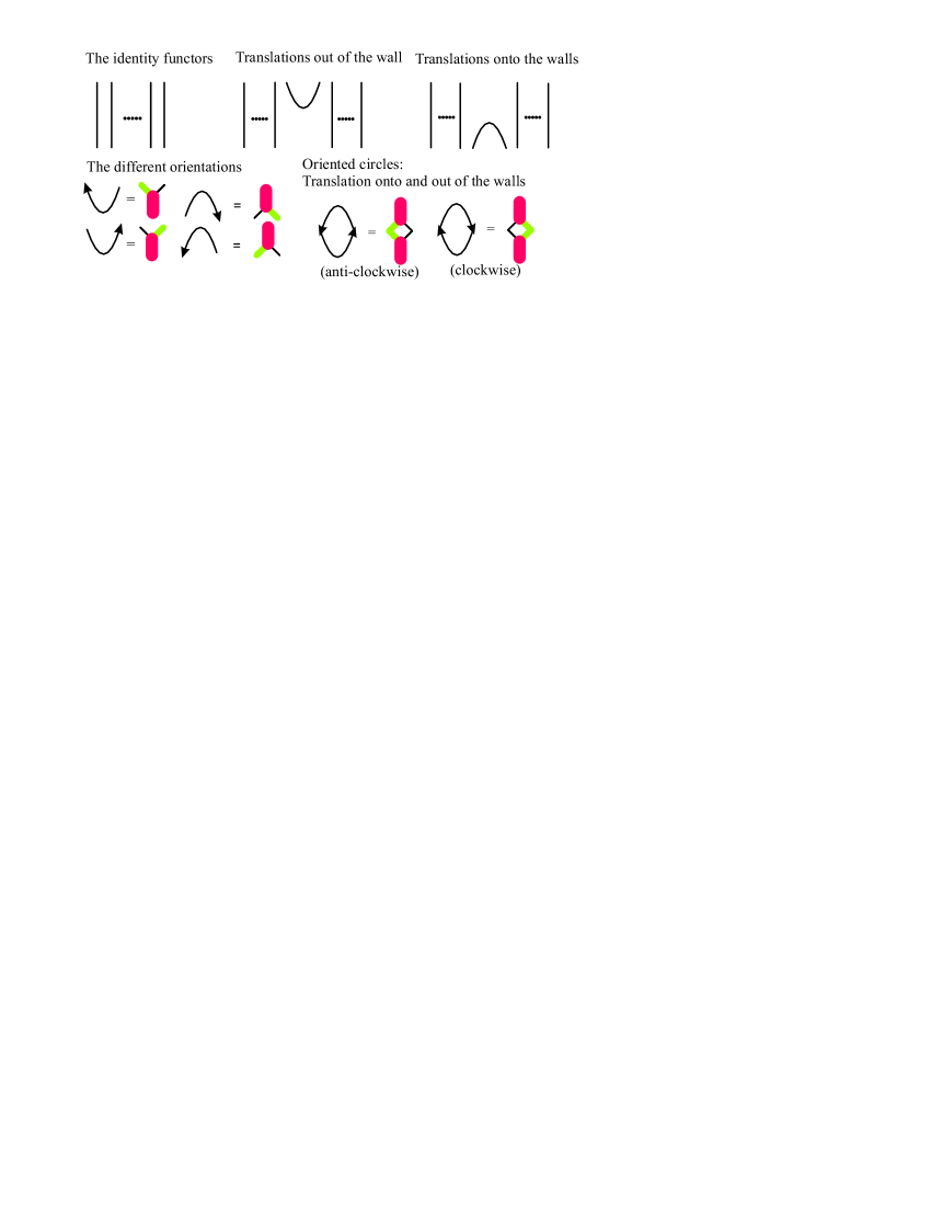
Figure 6. Crossingless elementary tangles and their associated functors

We want to use the previous paragraphs to construct a functor valued invariant of oriented tangles categorifying the quantum $\mathfrak{sl}_{k}$-invariants.

If ${\mathcal{A}}$ is an abelian category we denote by ${\mathcal{D}}^{b}({\mathcal{A}})$ the bounded derived category with shift functor $\llbracket\;\rrbracket$ such that $\llbracket 1\rrbracket$ shifts the complex one step to the right.

Recall now the definition of the tangle category ${\mathcal{T}}$ (see for example  [15], [17]). The objects are finite ${+,-}$-sequences, including the empty sequence; morphisms are the isotopy classes of oriented tangles. Here a plus indicates the orientation downwards, whereas a minus indicates the orientation upwards. The unoriented elementary tangles are depicted at the top of Figure 6. The first cup below would be a morphism from the emptyset to $(-,+)$, whereas the cup in the left lower corner is a morphism from the emptyset to $(+,-)$. Any morphism in ${\mathcal{T}}$ is a composition of oriented elementary morphisms.

For any object $a\in{\mathcal{T}}$ we define $|a|:=j+(k-1)i$ where $i$ is the number of pluses and $j$ the number of minuses in $a$. To an elementary morphism from $a$ to $b$ we associate a functor ${\mathcal{F}}:{\mathcal{D}}^{b}(\bigoplus_{\mu}{}^{\mathbb{Z}}{\mathcal{O}}(|a|)^{\mu})\rightarrow{\mathcal{D}}^{b}(\bigoplus_{\mu^{\prime}}{}^{\mathbb{Z}}{\mathcal{O}}(|b|)^{\mu^{\prime}})$, where $\mu$ and $\mu^{\prime}$ run through all partitions with at most $k$ parts, as follows:

Figure 7. Crossingless elementary tangles and their associated functors

1. To vertical strands we associate the identity functor (Figure 6) between the associated categories.

2. A cap diagram should first be replaced by a trivalent graph with labels $1$, $k-1$ and $k$, depending on its orientation, and as shown in Figure 6. To a cap diagram we associate the corresponding standard lift of translation functor onto the walls as defined in Section 4.1. The orientation determines the corresponding categories (Figure 6).

3. A cup diagram should first be replaced by a trivalent graph with labels $1$, $k-1$ and $k$, depending on its orientation, and as shown in Figure 6. To a cup diagram we associate then the corresponding standard lift of translation functor out of the walls as defined in Section 4.1.

4. Following [28], we associate to a positive crossing with upwards pointing arrows the corresponding left derived of the shuffling functor, but now shifted by $\langle-k\rangle\llbracket 1\rrbracket$. To a negative crossing we associate the right derived of the coshuffling functor shifted by $\langle k\rangle\llbracket-1\rrbracket$. In other words, we take the cone of the natural transformations as depicted in Figure 7, where the identity parts are concentrated in position zero of the complex. The natural transformations are both homogeneous of degree zero and arise as adjunction morphisms from translation on and out of the wall.

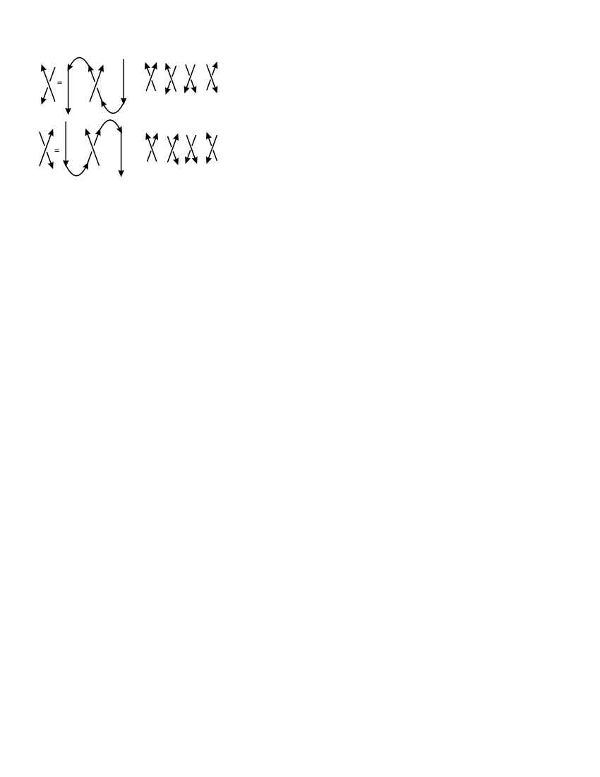
Figure 8. The functors associated with arbitrary crossings

To an arbitrary crossing we associate the functors given in Figure 8: We first consider the positive upwards pointing crossing and compose it with cap and cap as indicated to get the negative crossing pointing to the left. Repeating this process we get all the 4 crossings depicted to the right in the first row of Figure 8. Analogously we could start with the (negative) upwards pointing crossing and proceed as shown in the second row of Figure 8. This associates with each type of crossing a functor. To obtain Theorem 1.2 from the introduction we have to check the invariance under tangle moves.

6.1. The tangle moves

In Figure 9 we have depicted four pairs of functors. In the first pair, the functor $F$ on the RHS has been already defined and goes from the singularity $\nu=(1,k)$ to $\nu=(k,1)$. The corresponding categories can be identified via an Enright-Shelton equivalence ([8]). The following proposition ensures that under this identification the functor $F$ becomes isomorphic to the identity functor. We indicate the identifications to be made by slightly incline the arrow. Analogous statements hold for the remaining three functors shown in Figure 9. Hence the following result should be considered as a refined version of the isotopy relations of tangles:

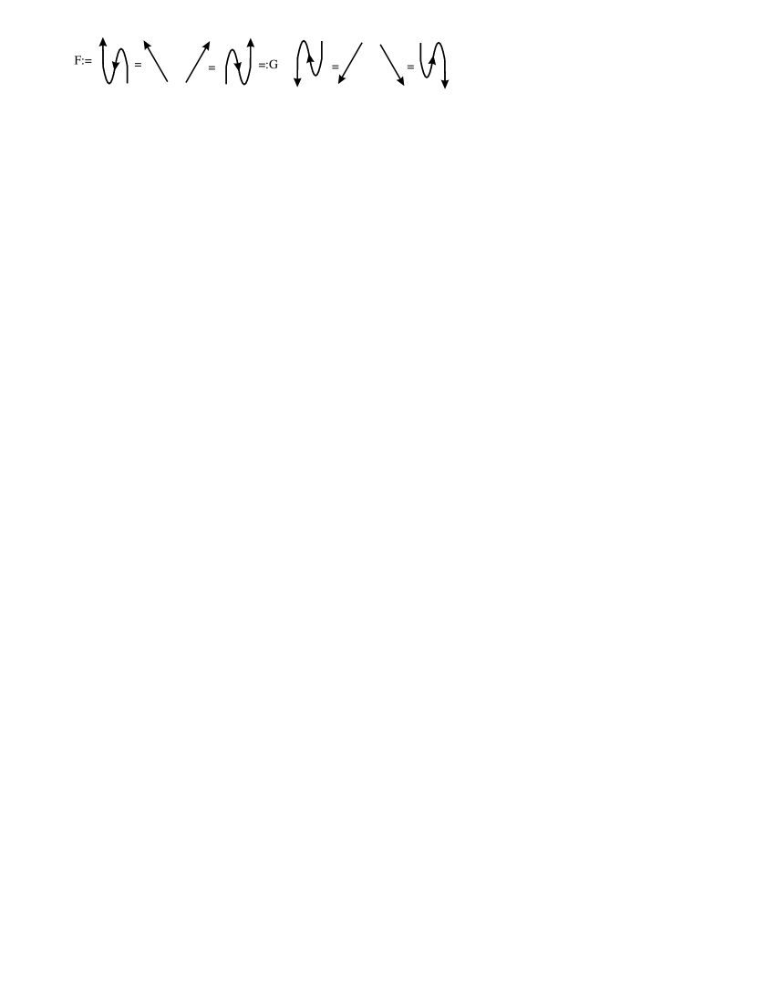
Figure 9. The 4 versions of the Isomorphism 1 of Tangles

Proposition 6.1 (Isomorphisms 1).

The functors depicted in Figure 9 are all equivalences of the corresponding categories. (The first two functors are mutually inverse, as so are the second two functors).

Proof.

Let $F^{\prime}=\theta^{(1,k)}_{(1,k-1,1)}\theta_{(k,1)}^{(1,k-1,1)}$ and $G^{\prime}=\theta^{(k,1)}_{(1,k-1,1)}\theta_{(1,k)}^{(1,k-1,1)}$ be the naively associated functors to the graphs of Figure 9. Combinatorially, the composition $G^{\prime}F^{\prime}$ is given as follows:

$$\begin{array}[]{l|l|l|l}(k,1)&(1,k-1,1)&(1,k)&(1,k-1,1)\\ \hline\cr e&A_{k-1}^{1}&A_{k-1}^{1}&A_{k-1}^{1}B_{2}^{k}\end{array}$$

Figure 10. The Verma flag of $F^{\prime}G^{\prime}\Delta(e)$

The braid relations in $S_{n}$ provide the equality

$$r\ldots 2\;1\;2\;3\;\ldots r=1\;2\ldots r(r-1)\ldots 2\;1$$

for any $1\leq r<n.$ Using these equalities one can show that $A_{k-1}^{1}B_{2}^{k}$ is of the form as depicted in Figure 10. The top line of the $i$-th box upstairs is in degree $i-1$, whereas the bottom line is always in degree $k-2$. The top line of each box downstairs is in degree $k-1$, whereas the bottom line of the $i$-th box is in degree $k-2+i$. We combine the $i$-th upstairs box with the $i+1$-th downstairs box.

Translating to $(k,1)$, any two combined boxes together represent (up to a shift in the grading) a copy of the projective module $P:=P(1\;2\;\ldots k)$. (Above or below each box we denoted the grading shift $\langle-j\rangle$ which occurs if we translate any element $x$ from the box to $(k,1)$ - one just has to remove the last $j$ elements from $x$ and shift by $-j$ in the grading). The only remaining element from the first downstairs box becomes a copy of $P(e)$. Altogether we get $G^{\prime}F^{\prime}\Delta(e)=[k-1]P\oplus P(e)$. The projective module $\theta_{k,1}^{(1^{k+1})}P$ corresponds to the following permutation (of $k+1$ letters)

$$x=\left(\begin{array}[tbh]{cccccccccccccc}1&2&3&\ldots&k-1&k&k+1\\ k+1&k&k-1&\ldots&3&2&1\end{array}\right)$$

Under the Robinson-Schensted correspondence this corresponds to a tableau with entries $1,2,\ldots,k+1$ in its first column. Fact 3 implies now $FG\cong\operatorname{id}_{(k,1)}$. We leave it to the reader to verify that $G^{\prime}F^{\prime}\Delta(e)\cong P(k\;(k-1)\ldots 1)\oplus\Delta(e)$, where the first summand translated out of the walls is $P(x)$, where $x$ is as above. Invoking again Fact 3, it follows $GF\cong\operatorname{id}_{(1,k)}$. Hence the functors $F$ and $G$ define mutually inverse equivalences of (the singular parabolic) categories in question. Similar calculations show that the remaining two functors are mutually inverse equivalences as well, we omit the details. ∎

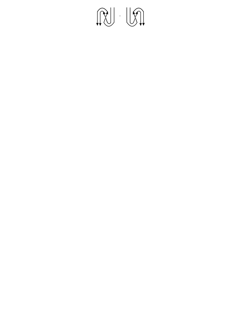
Figure 11. Isomorphism 2 of Tangles

Proposition 6.2.

The functors associated to the tangle diagrams depicted in Figure 11 are isomorphic.

As preparation we need to prove several small statements, formulated as Lemmas.

Lemma 6.3.

There is an isomorphisms of functors as shown in Figure 12.

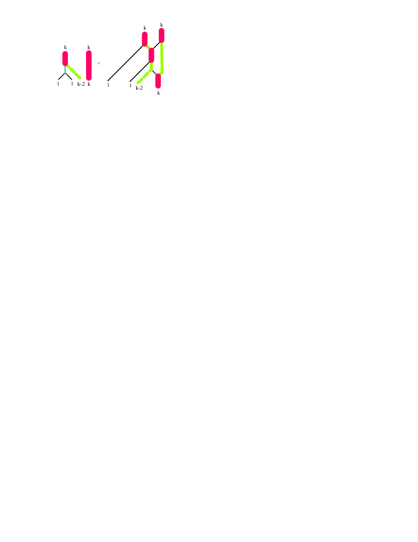
Figure 12. Step 1 in the proof of Proposition 6.2

Proof.

The proof is again completely combinatorial, so we leave out the details. The functor associated with the left hand side maps $\Delta(e)$ to $\Delta(e)$. The functor associated with the right hand side maps $\Delta(e)$ to a direct sum of $\Delta(e)$ and copies of $P:=P\left((2k-1)\ldots(k+1)2\ldots k\right)$. On the other hand $\theta_{(k,k)}^{(1^{2k})}P=P(x)$, where

$$x=\left(\begin{array}[tbh]{ccccccccccccccc}1&2&3&\ldots&k-1&k&k+1&k+2&\ldots&2k-1&2k\\ 2k&k&k-1&\ldots&3&1&2k-1&2k-2&\ldots&k+1&2\end{array}\right),$$

and so $x$ corresponds to a tableaux with the numbers $1,3,4,\ldots k,2k-1,2k$ in the first column, which means there are $k-1+2=k+1$ rows. The statement follows by applying Fact 3. ∎

Lemma 6.4.

There is an isomorphisms of functors as shown in Figure 13.

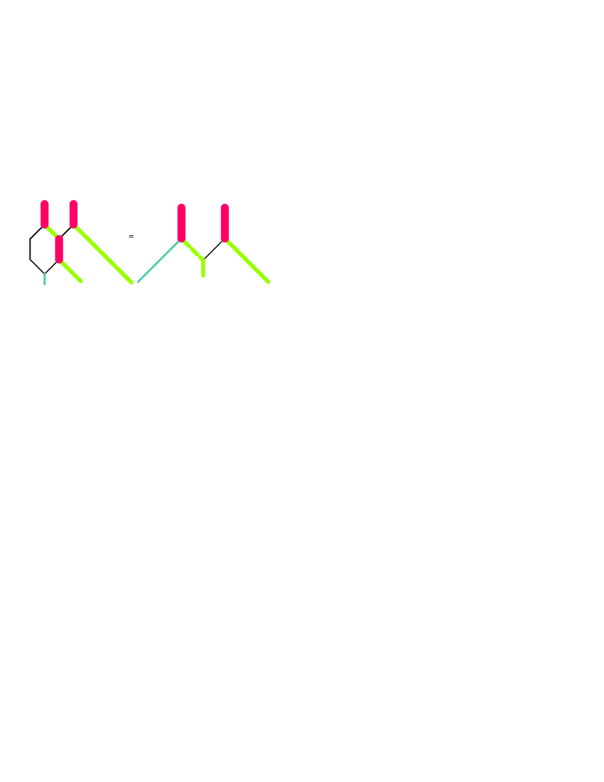
Figure 13. Step 2 in the proof of Proposition 6.2

Proof.

The proof is again completely combinatorial, so we leave out the details. The functor associated with the right hand side maps $\Delta(e)$ to $P(3\ldots k)$, whereas the functor associated with the left hand side maps $\Delta(e)$ to $P(12\ldots k)\oplus P(3\ldots k)$. Note that $\theta_{(k,k)}^{1^{2k}}P(12\ldots k)=P(x)$, where

$$x=\left(\begin{array}[tbh]{cccccccccccccc}1&2&\ldots&k&k+1&\ldots&2k-1&2k\\ k+1&k&\ldots&2&2k&\ldots&k+2&1\end{array}\right),$$

and so $x$ corresponds to a tableaux with the numbers $1,2,\ldots,k+1$ in the first column, which means there are $k+1$ rows. The statement follows. ∎

Proof of Proposition 6.2.

Let $F_{1}$ (resp. $F_{2}$) be the functor on the left (right) hand side of Figure 12. Let $G_{1}$ (resp. $G_{2}$) be the functor on the left (right) hand side of Figure 13. Fix any composition $\mu$ of $2k$ with at most $k$ parts and consider the functors

$$\begin{array}[thb]{lllllllll}H&:=&\theta_{(1,1,k-1,k-1)}^{(2,k-1,k-1)}:&&{\mathcal{O}}_{(1,1,k-1,k-1)}^{\mu}&\rightarrow&{\mathcal{O}}_{(2,k-1,k-1)}^{\mu}\\ J&:=&\theta^{(1,1,k-2,k)}_{(1,1,k-2,1,k-1)}\theta_{(1,1,k-1,k-1)}^{(1,1,k-2,1,k-1)}:&&{\mathcal{O}}_{(1,1,k-1,k-1)}^{\mu}&\rightarrow&{\mathcal{O}}_{(1,1,k-2,k)}^{\mu}\end{array}$$

Then we have isomorphisms of functors as follows:

$$G_{1}H\cong G_{2}H\cong F_{1}J\cong F_{2}J.$$

This follows directly from the Lemmas 12 and 13 by drawing pictures. Using Proposition 9, Figure 9 we see that $F_{2}J$ is isomorphic to the functor given by the vertically reflected diagram. From this it follows that we have an isomorphism of functors as in Figure 11, but the crossings replaced by . Now one has just to take the Cone of the corresponding adjunction morphism. Up to a scalar, there is a unique morphism with the correct degree. The statement of the Proposition follows by applying Fact 3. ∎

Proposition 6.5 (Reidemeister 2 and 3).

The functors associated to the positive and negative upwards pointing crossings are mutually inverse equivalences and satisfy the braid relations.

Proof.

This is a standard fact, see for example [22]. ∎

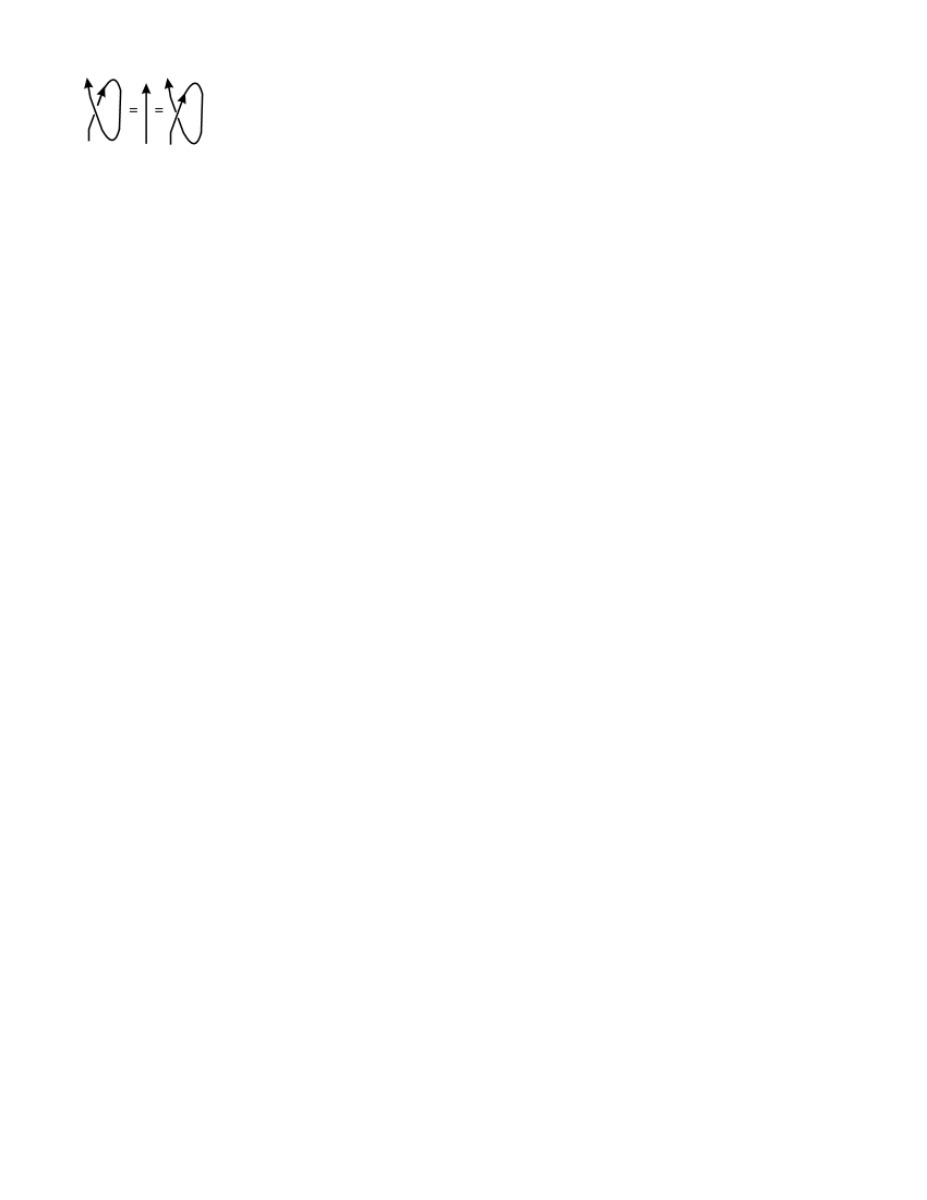
Figure 14. Reidemeister 1

Proposition 6.6 (Reidemeister1).

The three functors associated to the tangle diagrams in Figure 14 are isomorphic.

Proof.

The functors in question are going from the singularity $(1,k)$ to the singularity $(1,k)$. Recall the definition of the functor associated to the crossings.

Let us first give a short explanation why one might expect the claimed isomorphisms: From the relations in Figures 3 and Figure 2 the functor on the left hand side of Figure 14 is, up to an overall shift by $\langle-k\rangle$, the Cone of a morphism

$$\gamma:\quad[k]\operatorname{id}\langle 1\rangle\longrightarrow[k-1]\operatorname{id},$$

sitting in cohomological degree zero and $1$. There is the obvious surjection

$$(q^{k}+q^{k-2}+q^{k-4}+\ldots+q^{4-k}+q^{2-k})\operatorname{id}\rightarrow(q^{k-2}+q^{k-4}+\ldots+q^{4-k}+q^{2-k})\operatorname{id}$$

which identifies the same summands and has kernel $q^{k}\operatorname{id}$, so that we expect the second isomorphism of Figure 14 (and similarly the first one). To prove the statement we have to understand the morphism $\gamma$ better.

The adjunction morphism $\alpha:\theta_{(1,k)}^{(1,1,k-1)}\rightarrow\theta_{2,k-1}^{1,1,k-1}\theta_{1,1,k-1}^{2,k-1}\theta_{(1,k)}^{(1,1,k-1)}$ is injective for any module with Verma flag, in particular for Verma modules and projectives. From the proof of Proposition 5.2 we see that the image of the adjunction morphism applied to $\Delta(e)$ is a module with Verma subquotients given by $qA_{2}^{k}$, $q^{k}e$. Hence $\gamma^{\prime}:=\theta_{(1,1,k-1)}^{(1,k)}(\alpha)_{\Delta(e)}$ surjects onto the $[k-1]$ copies of $\Delta(e)$, and defines a split

$$\theta^{(1,k)}_{(1,1,k-1)}\theta_{(1,k)}^{(1,1,k-1)}\cong F^{\prime}\oplus[k-1]\operatorname{id}$$

for some projective functor $F^{\prime}$. Thanks to Proposition 5.1 we have $F^{\prime}\cong\operatorname{id}\langle k\rangle$. Now, if we restrict to the parabolic subcategories with at most $k$ parts, then $\gamma^{\prime}$ induces the surjection with kernel the identity functor shifted up by $k$ in the degree. Putting the overall shift back into the picture, we obtain the second isomorphism. The first isomorphism can be proved analogously or by observing that these are just the adjoint functors. ∎

Proposition 6.7.

The functors associated to the tangle diagrams in Figure 15 satisfy the displayed isomorphisms.

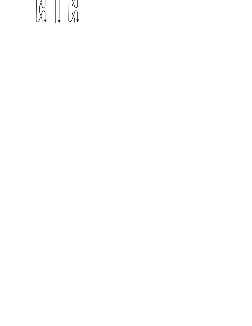
Figure 15. Isomorphisms of Tangles

Proof.

The right half of Figure 15 is just the reflection in a vertical line of the diagrams in Figure 15. Now there is an isomorphism of the Lie algebra $\mathfrak{gl}_{n}$ given by the obvious involution of the Dynkin diagram which swaps the $i$-th with the $n-1-i$-th node. This isomorphism defines an auto-equivalence of the category ${\mathcal{O}}$ for $\mathfrak{gl}_{n}$ which identifies ${}^{\mathbb{Z}}{\mathcal{O}}(n)_{\nu}^{\mu}$ with ${}^{\mathbb{Z}}{\mathcal{O}}_{\tilde{\nu}}^{\tilde{\mu}}$, where the partition are “reflected in a vertical line”. Under this automorphism the functors displayed on the left half of Figure 15 correspond to the functors displayed on the right half, so that it is enough to prove the first two isomorphisms. Consider first the diagram on the left hand side together with the following functors

$$F:=\theta_{(k,1,k-1)}^{(k-1,1,1,k-1)}, \hat{F}:=\theta^{(k,1,k-1)}_{(k-1,1,1,k-1)}$$

$$H:=\theta_{(k-1,1,1,k-1)}^{(k-1,1,k)}, \hat{H}:=\theta^{(k-1,1,1,k-1)}_{(k-1,1,k)},$$

$$\theta:=\theta^{(k-1,1,1,k-1)}_{(k-1,2,k-1)}\theta_{(k-1,1,1,k-1)}^{(k-1,2,k-1)}$$

$$G:=\operatorname{Cone}(\theta\longrightarrow\operatorname{id}\langle-1\rangle)\langle k\rangle, \hat{G}:=\operatorname{Cone}(\operatorname{id}\langle 1\rangle\longrightarrow\theta)\llbracket 1\rrbracket\langle-k\rangle,$$

The relation we want to verify says exactly that after restricting to parabolics with at most $k$ parts, the functors $\Phi_{1}:=\hat{F}\,\hat{G}\,\hat{H}$ and $\Phi_{2}:=H\,G\,F$ are inverse to each other.

Directly from the definitions it follows, that the composition $\Phi_{1}\Phi_{2}$ is given by the the following complex of functors:

$$\hat{F}\hat{H}\,H\,\theta\,F\langle 1\rangle\longrightarrow\hat{F}\,\theta\,\hat{H}\,H\,\theta\,F\oplus\hat{F}\hat{H}\,H\,F\longrightarrow\hat{F}\,\theta\,\hat{H}\,H\,F\langle-1\rangle.$$

Here the first map is $\left(\begin{array}[]{c}\hat{F}(\beta)_{\hat{H}H\theta F}\\ \hat{F}\hat{H}H(\alpha)_{F}\end{array}\right)$, and the second is $\big{(}\hat{F}\theta\hat{H}H(\alpha)_{F},-\hat{F}(\beta)_{\hat{H}HF}\big{)}$, where $\alpha$ is the adjunction morphism $\theta\rightarrow\operatorname{id}\langle-1\rangle$ and $\beta$ the adjunction morphism $\operatorname{id}\langle 1\rangle\rightarrow\theta$.

Using now the Relations (I), (III) and (IV) (Figures 1, 3, 4) the restrictions of the functors to any parabolic with at most $k$ parts gives rise to the complex

(6.6) $$[k-1]J\langle 1\rangle\longrightarrow(\operatorname{id}\oplus[k-2]J)\oplus[k]J\longrightarrow[k-1]J\langle-1\rangle$$

where $J$ is the restriction of the functor $\theta^{(k,k-1,1)}_{(k,k)}\theta_{(k,k-1,1)}^{(k,k)}$. As in Proposition 6.6 we deduce that the first map is an inclusion and the second map is a surjection so that the functor $[k-1]J\langle-1\rangle$ splits off as a direct summand and (6.6) is quasi-isomorphic to

(6.7) $$0\rightarrow[k-1]J\langle 1\rangle\overset{\gamma}{\longrightarrow}\operatorname{id}\oplus[k-1]J\rightarrow 0.$$

Denote by $\kappa_{1}:\operatorname{id}\oplus[k-1]J\rightarrow[k-1]J$ the projection. We claim that $\kappa_{1}\gamma$ is an isomorphism.

Indeed, assume that this is not the case. Let $P(w)$ be an indecomposable projective, different from the dominant Verma module $\Delta(e)$. Then the Verma flag of $P(w)$ contains, as a submodule, the copy of $\Delta(e)$ which corresponds to the inclusion $\Delta(w)\hookrightarrow\Delta(e)$. The socle of this submodule is in the kernel of any non-invertible homomorphism $f:P(w)\rightarrow P(w)$ and any homomorphism $g:P(w)\rightarrow\Delta(e)$. Thus it is in the kernel of $\gamma_{\Delta(e)}$, which contradics the injectivity of $\gamma$.

Let $\kappa_{2}:\operatorname{id}\oplus[k-1]J\rightarrow\operatorname{id}$ be the projection. In particular, $\gamma=\left(\begin{array}[]{c}\kappa_{2}\gamma\\ \kappa_{1}\gamma\end{array}\right)$. Now the map $(\mathrm{id},-\kappa_{2}\gamma(\kappa_{1}\gamma)^{-1}):\operatorname{id}\oplus[k-1]J\rightarrow\operatorname{id}$ satisfies $(\mathrm{id},-\kappa_{2}\gamma(\kappa_{1}\gamma)^{-1})\gamma=0$ and hence defines a quasi-isomorphism from (6.7) to the complex $0\rightarrow\operatorname{id}\rightarrow 0$, which represents the identity functor. This proves the first isomorphism. The second can be deduced analogously. Alternatively one could deduce it by adjointness properties. ∎

To summarise: Theorem 1.2 from the introduction holds.

7. Cohomology rings, natural transformations and foams

In this final section we indicate how to extend our functorial invariant of trivalent graphs to an invariant of trivalent graphs and foams, and also explain the connection with [16]. Conjecturally our setup actually gives the representation theoretical background for the very recent generalisation [19] of [16] to arbitrary $k$.

Roughly speaking, a foam is a morphism between certain trivalent graphs (for a precise definition see [16], [20], [19]). Khovanov associated to each special trivalent graph a graded vector space and to any foam a homogeneous linear map of degree being the degree of the foam. In the following we want to indicate how this construction emerges naturally from our picture by restricting the functors to the non-parabolic part and applying some Soergel’s combinatorial functor $\mathbb{V}$. In the following we assume that the reader is familiar with [16].

7.1. Natural transformation associated with basic foams

Apart from the identity morphisms, un-dotted foams are compositions of elementary foams as depicted in Figure 16.

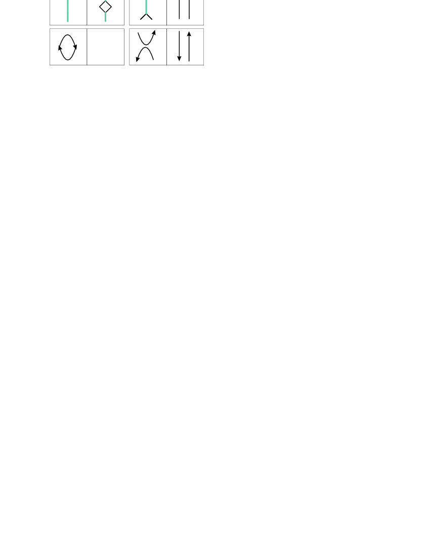
Figure 16. Basic Foams correspond to basic natural transformations, homogeneous of degree $-1$, $1$, $-2$, $2$ respectively.

Each rectangle should be read from the left to the right, as well as from the right to the left; giving rise to two basic foams. Additionally, both possible orientation should be considered in the last two cases. For each graph appearing as the boundary of a foam, we have the associated functor (Section 5). We assign now to each basic foam a natural transformation, all of them will be just adjunction morphisms:

First row: We associate the adjunction morphism $\beta_{1}$ from the identity to the composition $\theta_{(1,1)}^{(2)}\theta_{(2)}^{(1,1)}$, and $\beta_{2}$ vice versa. $\beta_{1}$ and $\beta_{2}$ are homogeneous of degree $-1$ ([27, Theorem 8.4]). Thanks to ([27, Remarks 3.8 c)]) we have adjunction morphisms $\alpha_{1}:\operatorname{id}\rightarrow\theta_{(2)}^{(1,1)}\theta_{(1,1)}^{(2)}$ and $\alpha_{2}:\theta_{(2)}^{(1,1)}\theta_{(1,1)}^{(2)}\rightarrow\operatorname{id}$, both homogeneous of degree $1$. A priori, they are unique up to a non-zero scalar - which we want to choose such that Lemma 7.2 and Lemma 7.3 below hold; the same will apply to all the other adjunction morphisms. These are the natural transformations we associate to the two foams given by the first diagram.

The second row: Recall that we associated to a circle the composition of translation out of the walls and onto the walls as depicted in Figure 6. Hence we have the obvious adjunction morphisms $\gamma_{1}$ from a clockwise circle, $\gamma_{2}$ from an anticlockwise circle, $\gamma_{3}$ to a clockwise circle, $\gamma_{4}$ to an anticlockwise circle. They are all homogeneous of degree $1-k$. This follows from the adjunction $(\theta^{(i,j)}_{(k)},\theta^{(k)}_{(i,j)})$, where $(i,j)\in\{(1,k-1),(k-1,1)\langle 1-k\rangle\}$ (a special case of [9, Proposition 4.2]). The adjunction morphisms $\delta_{1}:\theta_{(3)}^{(2,1)}\theta_{(2,1)}^{(3)}\rightarrow\operatorname{id}$, $\delta_{1}^{\prime}:\theta_{(3)}^{(1,2)}\theta_{(1,2)}^{(3)}\rightarrow\operatorname{id}$ and $\delta_{2}:\operatorname{id}\rightarrow\operatorname{\theta}_{(3)}^{(2,1)}\theta_{(2,1)}^{(3)}$, $\delta_{2}^{\prime}:\operatorname{id}\rightarrow\operatorname{\theta}_{(3)}^{(1,2)}\theta_{(1,2)}^{(3)}$, are homogeneous of degree $k-1$ (by the combinatorics of Section 4).

From now on we stick to the case $k=3$ and illustrate the connection to [16]. Denote by $\deg{\mathtt{F}}$ the degree of a basic foam $\mathtt{F}$. From the definition it follows:

Lemma 7.1.

Let $k=3$. For a basic foam $\mathtt{F}$ let $\phi_{\mathtt{F}}$ be the associated natural transformation as defined above. Then $\operatorname{deg}(\mathtt{F})=\operatorname{deg}(\phi_{\mathtt{F}}).$

Apart from the basic foams we need the so-called theta foams. Theta-foams (Figure 17) are obtained by gluing three oriented disks along their boundaries (their orientations must coincide).

Figure 17. Examples of Theta foams with all the non-trivial evaluations

Dots will correspond to multiplication with a certain element of degree two in the centre of the category. This will be exactly as in [16] and [19]. To explain this connection we have to bring cohomology rings of partial flag varieties into the picture.

7.2. The cohomology of flag varieties

Recall the following result of Soergel: The category ${}^{\mathbb{Z}}{\mathcal{O}}(n)_{\lambda}$ (for $\lambda$ a partition of $n$) has one indecomposable projective-injective module $P_{\lambda}$ with head concentrated in degree zero. We have Soergel’s functor

$$\mathbb{V}=\operatorname{Hom}_{{\mathcal{O}}}(P(\lambda),_{-}):{}^{\mathbb{Z}}{\mathcal{O}}(n)_{\lambda}\longrightarrow\operatorname{gmod}-\operatorname{End}_{{\mathcal{O}}}(P_{\lambda}).$$

By Soergel’s Endomorphismensatz ([25]) we know that $\operatorname{End}_{{\mathcal{O}}}(P_{\lambda})$ is isomorphic (as a graded ring) to the cohomology ring (with complex coefficients) of the associated partial flag variety ${\mathcal{F}}_{\lambda}$, where the dimensions of the subquotients are $\{\lambda_{i}\}_{i>0}$.

For instance $\operatorname{End}(P_{(1,1)})\cong H^{*}({\mathcal{F}}_{(1,1)})\cong\mathbb{C}[x]/(x^{2})$. If we choose $\lambda=(3)$, then we just get the cohomology $\mathbb{C}$ of a point, whereas $\operatorname{End}_{{\mathcal{O}}}(P_{\lambda})\cong H^{*}(\mathbb{P}^{2})\cong\mathbb{C}[x]/(x^{3})$ if $\lambda=(2,1)$ or $\lambda=(1,2)$. In each case, $x$ is of degree two. If we choose the reversed standard orientation on $\mathbb{P}^{2}$, then the cohomology ring ${\mathcal{A}}:=\mathbb{C}[x]/(x^{3})$ comes along ([16]) with the trace form $\operatorname{Tr}(x^{i})=-1\delta_{2,i}$ and the comultiplication

$$\Delta(1)=-(1\otimes x^{2}+x\otimes x+x^{2}\otimes 1),\quad\Delta(x)=-(x\otimes x^{2}+x^{2}\otimes x),\quad\Delta(x^{2})=-x^{2}\otimes x^{2}.$$

We choose the basis $X_{(1)}=1,X_{(2)}=x,X_{(3)}=x^{2}$ of ${\mathcal{A}}$ and denote by $X^{(1)}$, $X^{(2)}$, $X^{(3)}$ its dual basis with respect to $\operatorname{Tr}$.

Finally, the cohomology ring $C:=H^{*}({\mathcal{F}}_{(1,1,1)})$ is isomorphic to the polynomial ring $\mathbb{C}[X_{1},X_{2},X_{3}]$ modulo the ideal generated by the elementary symmetric polynomials. There is the trace function $\operatorname{Tr}:C\rightarrow\mathbb{C}$ which maps $X_{1}X_{2}^{2}$ to $1$.

7.3. The bridge

The functor $\mathbb{V}$ connects category ${\mathcal{O}}$ and modules over cohomology rings of flag varieties: The functor $\theta_{(2)}^{(1,1)}\theta^{(2)}_{(1,1)}:{}^{\mathbb{Z}}{\mathcal{O}}(2)_{(1,1)}\rightarrow{}^{\mathbb{Z}}{\mathcal{O}}(2)_{(1,1)}$ corresponds ([25], [27]) under $\mathbb{V}$ to the functor

$$\bullet\otimes_{\mathbb{C}}\mathbb{C}[x]/(x^{2})\langle-1\rangle:\quad\operatorname{gmod}-\mathbb{C}[x]/(x^{2})\rightarrow\operatorname{gmod}-\mathbb{C}[x]/(x^{2}).$$

Lemma 7.2.

Under the above correspondence the natural transformations $\alpha_{1}$, $\alpha_{2}$ become the multiplication $\mathbb{V}(\alpha_{1})_{N}:(N\otimes_{\mathbb{C}}\mathbb{C}[x]/(x^{2})\langle-1\rangle)\langle 1\rangle\rightarrow N$, $n\otimes c\mapsto nc$ and the comultiplication $\mathbb{V}(\alpha_{2})_{N}:N\langle 1\rangle\rightarrow N\otimes_{\mathbb{C}}\mathbb{C}[x]/(x^{2})\langle-1\rangle$, $n\mapsto x\otimes n+1\otimes xn$ respectively.

Proof.

See [28, Lemma 8.2]. ∎

Similarly, the functor $\theta^{(2)}_{(1,1)}\theta_{(2)}^{(1,1)}:{}^{\mathbb{Z}}{\mathcal{O}}(2)_{(2)}\rightarrow{}^{\mathbb{Z}}{\mathcal{O}}(2)_{(2)}$ corresponds under $\mathbb{V}$ to the functor

(7.1) $$\bullet\otimes_{\mathbb{C}}\mathbb{C}[x]/(x^{2})\langle-1\rangle\cong\operatorname{id}\langle 1\rangle\oplus\operatorname{id}\langle-1\rangle:\quad\operatorname{gmod}-\mathbb{C}\rightarrow\operatorname{gmod}-\mathbb{C}.$$

Lemma 7.3.

With the above definitions, for every graded $\mathbb{C}$-module $N$ we have $\mathbb{V}(\beta_{1})_{N}:N\langle-1\rangle\rightarrow N\otimes_{\mathbb{C}}\mathbb{C}[x]/(x^{2})\langle-1\rangle,$ $n\mapsto n\otimes 1$ and we further have the following: $\mathbb{V}(\beta_{2})_{N}:(N\otimes_{\mathbb{C}}\mathbb{C}[x]/(x^{2})\langle-1\rangle)\langle-1\rangle\rightarrow N,$ $n\otimes c\mapsto\operatorname{Tr}(c)n$. Under the isomorphism (7.1) we just get the projection and inclusion morphisms of degree $-1$.

Proof.

Since the source and target categories of the functors are semi-simple, there is only one (up to scalar) possible map of the correct degree in each case. ∎

Now consider the functor $\theta_{(3)}^{(2,1)}\theta^{(3)}_{(2,1)}:{}^{\mathbb{Z}}{\mathcal{O}}(3)_{(2,1)}\rightarrow{}^{\mathbb{Z}}{\mathcal{O}}(3)_{(2,1)}.$ Under the functor $\mathbb{V}$ this corresponds to the functor

(7.2) $$\bullet\otimes_{\mathbb{C}}\mathbb{C}[x]/(x^{3})\langle-2\rangle \cong \bullet\otimes_{\mathbb{C}}{\mathcal{A}}\langle-2\rangle$$

([9, 3.4]). Because of Soergel’s double centralizer property with respect to the antidominand projective module, a natural transformation between projective functors is already determined by its value on the antidominant projective module (by argumens similar to e.g. [23, Lemma 5.1]). Hence the following Lemma is useful:

Lemma 7.4.

Under the functor $\mathbb{V}$ we have the following correspondences:

• Evaluated at the antidominant projective module $P(21)$ or $P(12)$, the natural transformations $\delta_{1}$ and $\delta_{1}^{\prime}$ correspond to the multiplication morphism $m:({\mathcal{A}}\otimes{\mathcal{A}}\langle-2\rangle)\langle 2\rangle\rightarrow{\mathcal{A}}$, whereas $\delta_{2}$ and $\delta_{2}^{\prime}$ corresponds to the comultiplication morphism $\Delta:{\mathcal{A}}\langle 2\rangle\rightarrow{\mathcal{A}}\otimes{\mathcal{A}}\langle-2\rangle$.

• Evaluated at the dominant Verma module $\Delta(e)$, we get for $\delta_{1}$ and $\delta_{1}^{\prime}$ the induced multiplication morphism $\overline{m}:(\mathbb{C}\otimes{\mathcal{A}}\langle-2\rangle)\langle 2\rangle\rightarrow\mathbb{C}$, and for $\delta_{1}$ and $\delta_{1}^{\prime}$ the induced comultiplication morphism $\overline{\Delta}:\mathbb{C}\langle 2\rangle\rightarrow\mathbb{C}\otimes{\mathcal{A}}\langle-2\rangle$.

Proof.

Note first that we have $\mathbb{V}\theta_{(3)}^{(2,1)}\theta_{(2,1)}^{(3)}P(21)\cong{\mathcal{A}}\otimes{\mathcal{A}}\langle-2\rangle$, and similarly $\mathbb{V}\theta_{(3)}^{(1,2)}\theta_{(1,2)}^{(3)}P(12)\cong{\mathcal{A}}\otimes{\mathcal{A}}\langle-2\rangle$ by (7.2); whereas $\mathbb{V}\theta_{(3)}^{(2,1)}\theta_{(2,1)}^{(3)}\Delta(e)\cong\mathbb{C}\otimes{\mathcal{A}}\langle-2\rangle$, and similarly $\mathbb{V}\theta_{(3)}^{(1,2)}\theta_{(1,2)}^{(3)}\Delta(e)\cong\mathbb{C}\otimes{\mathcal{A}}\langle-2\rangle$. Frobenius reciprocity provides a natural isomorphism of the form

$$\operatorname{Hom}_{\operatorname{gmod}-{\mathcal{A}}}(N\otimes{\mathcal{A}},N)\cong\operatorname{Hom}_{\operatorname{gmod}-\mathbb{C}}(N,N)$$

mapping $f$ to $\hat{f}$, where $\hat{f}(n)=f(1\otimes n)$ for any graded right ${\mathcal{A}}$-module $N$ and $n\in N$. In particular, $\hat{m}$ is the identity map which implies half of the statement.

Denote by $X^{*}$ the graded vector space dual of $X$. Then there is an isomorphism of graded right ${\mathcal{A}}$-modules as follows:

$$\gamma:\quad(N\otimes{\mathcal{A}})^{*} \cong N^{*}\otimes{\mathcal{A}},\quad g\mapsto\sum_{i=1}^{3}g_{i}\otimes X^{(i)},\quad\widetilde{f\otimes c}\mapsfrom f\otimes c,$$

where $g_{i}(n)=g(n\otimes X_{(i)})$ and $\widetilde{f\otimes c}(n\otimes d)=\operatorname{Tr}(cd)f(n)$ for $n\in N$, $c,d\in{\mathcal{A}}$. The second adjunction morphism is then the chain of isomorphisms

$$\operatorname{Hom}_{\operatorname{gmod}-\mathbb{C}}(N,N) \cong \operatorname{Hom}_{\operatorname{gmod}-\mathbb{C}}(N^{*},N^{*})\cong\operatorname{Hom}_{\operatorname{gmod}-{\mathcal{A}}}(N^{*}\otimes{\mathcal{A}},N^{*})$$

$$\cong \operatorname{Hom}_{\operatorname{gmod}-{\mathcal{A}}}((N\otimes{\mathcal{A}})^{*},N^{*})\cong\operatorname{Hom}_{\operatorname{gmod}-{\mathcal{A}}}(N,N\otimes{\mathcal{A}}).$$

The first isomorphism here is the duality, the second the adjunction from above, then we invoke the isomorphism $\gamma$ and finally the duality again. It is now an easy direct calculation to verify the claim. ∎

Lemma 7.5.

Under the functor $\mathbb{V}$ for every graded $\mathbb{C}$-module $N$ we have the following: $\mathbb{V}(\gamma_{1})_{N}:N\langle-2\rangle\rightarrow N\otimes_{\mathbb{C}}\mathbb{C}[x]/(x^{3})\langle-2\rangle,n\mapsto n\otimes 1$ and further we have $\mathbb{V}(\gamma_{2})_{N}:(N\otimes_{\mathbb{C}}\mathbb{C}[x]/(x^{3})\langle-2\rangle)\langle-2\rangle\rightarrow N,n\otimes c\mapsto\operatorname{Tr}(c)n$. Under the isomorphism from Figure 1 we just get the inclusion and projection morphisms of degree $-2$. The same holds for $\gamma_{1}^{\prime}$ and $\gamma_{2}^{\prime}$.

7.3.1. Dots on basic foams

We still have to explain what to do with dots on basic foams. Under the functor $\mathbb{V}$ any dot just corresponds to multiplication with the variable $x$. By Soergel’s Struktursatz this means that we multiply the natural transformation with a certain element of the centre of one of the involved categories ([25], [23]). To make this explicit, consider the functors $F:=\theta_{(3)}^{(2,1)}\theta^{(3)}_{(2,1)}$ and $G:=\theta_{(3)}^{(1,2)}\theta^{(3)}_{(1,2)}$. A natural transformation $f:F\rightarrow F$ (or $g:G\rightarrow G$) is uniquely determined by $\mathbb{V}(f):\mathbb{V}F\Delta(e)\rightarrow\mathbb{V}F\Delta(e)$ (or $\mathbb{V}(g):\mathbb{V}G\Delta(e)\rightarrow\mathbb{V}G\Delta(e)$) (because ${\mathcal{O}}(3)_{(3)}$ is semisimple).

Choosing for $f$ and $g$ the identity morphism, we have $\mathbb{V}(f),\mathbb{V}(g):{\mathcal{A}}\rightarrow{\mathcal{A}}$, and one checks directly that the surgery operation from Figure 18 decomposes them as follows:

$$-\operatorname{id} = m_{x}\circ m_{x}\circ\delta_{2}\circ\delta_{1}+m_{x}\circ\delta_{2}\circ\delta_{1}\circ m_{x}+\delta_{2}\circ\delta_{1}\circ m_{x}\circ m_{x}$$

$$-\operatorname{id} = m_{x}\circ m_{x}\circ\delta_{2}^{\prime}\circ\delta_{1}^{\prime}+m_{x}\circ\delta_{2}^{\prime}\circ\delta_{1}^{\prime}\circ m_{x}+\delta_{2}^{\prime}\circ\delta_{1}^{\prime}\circ m_{x}\circ m_{x}$$

where $m_{x}$ is the multiplication with $x$ which we associate with a dot.

Figure 18. The surgery relation decomposes the identity morphisms

7.3.2. Theta foams

We have to associate to each theta foam a natural transformation from the identity functor on ${}^{\mathbb{Z}}{\mathcal{O}}(3)_{(3)}$ to itself. To a theta foam with $d_{i}$ dots on the $i$-th disk we associate the natural transformation which corresponds under the functor $\mathbb{V}$ to the map $\mathbb{C}\rightarrow\mathbb{C}$, $z\mapsto\operatorname{Tr}(X_{1}^{d_{1}}X_{2}^{d_{2}}X_{3}^{d_{3}})z$. In particular, corresponding to the three discs (the equatorial, the upper hemisphere and the lower hemisphere) there are three embeddings of ${\mathcal{A}}$ into $C$, namely $x\mapsto X_{1}$, $x\mapsto X_{2}$ and $x\mapsto X_{3}$ and we apply the usual rule for the dots.

Let $\mathtt{F}$ be a basic foam with input boundary $D_{F_{1}}$ and output boundary $D_{F_{2}}$. Let $F_{1}$, $F_{2}$ be the corresponding functors as assigned in Section 4 and $G_{1}$, $G_{2}$ the associated graded vector spaces in [16]. Assigned to $\mathtt{F}$ we have $\phi_{\mathtt{F}}:F_{1}\rightarrow F_{2}$ and also a linear map $g:G_{1}\rightarrow G_{2}$ from [16]. Let $\overline{F}_{1}$, $\overline{F}_{2}$ and $\overline{\phi_{\mathtt{F}}}$ be the restrictions to the non-parabolic summand. The following result is now easily verified:

Proposition 7.6.

1. The above assignments define a functor from the category of prefoams as defined in [16] to the category of graded projective functors associated with intertwiners and natural transformations between them.

2. There are isomorphism $\mathbb{V}\overline{F}_{i}\Delta(e)\cong G_{i}$, $i=1,2$, of graded vector spaces under which $\mathbb{V}\overline{\phi_{\mathtt{F}}}$ corresponds to $g$.

In particular, the approach of [16] follows directly from our setup by restriction. Note that we really loose some information here, since we evaluate the natural transformation on the dominant Verma module (instead of on the antidominant projective which would keep all the information). On the other hand, we restricted to a direct summand. This is irrelevant for the quality of the invariant, but only carries the information of the zero weight space in our original $\mathfrak{sl}(k)$-modules $X^{\nu}$.

Conjecture 7.7.

The obvious generalisation of our construction for general $k$ gives rise to the Mackaay-Stosic-Vaz homology ([19]) and hence to the Khovanov-Rozansky homology [18].

A verification of this conjecture would in particular imply a very nice description of the interplay of natural transformations between projective functors in terms of Schur polynomials, based on [19].

7.4. Speculations on web bases and dual canonical bases

In Section 4 we associated to each special intertwiner or web diagram a certain projective functor. In the case $k=2$ the web bases coincides with the Temperley-Lieb algebra basis which agrees with Lusztig’s canonical basis ([10]). One can show that the associated functors are all indecomposable ([28]). This is however just pure accident and very special for $k=2$. The answer to the following question might shed some light on the relationship in general:

Question. Is it true that the transformation matrix between the web basis and the canonical basis describes the decomposition of the functors assigned to webs into a direct sum of indecomposable functors?

To answer this question one has to improve the categorification presented in the present paper, to include more general intertwiners, and then connect it with the results on dual canonical bases from [11], and the more general results [6]. Since there is no classification of indecomposable projective functors for parabolic categories we expect that finding an answer to this question might be quite hard.

References

- [1] H. H. Andersen and C. Stroppel. Twisting functors on . Represent. Theory, 7:681–699, 2003.
- [2] A. Beilinson, V. Ginzburg, and W. Soergel. Koszul duality patterns in representation theory. J. Amer. Math. Soc., 9(2):473–527, 1996.
- [3] I. N. Bernstein, I. M. Gel′fand, and S. I. Gel′fand. A certain category of -modules. Funkcional. Anal. i Priložen., 10(2):1–8, 1976.
- [4] J. Bernstein, I. Frenkel, and M. Khovanov. A categorification of the Temperley-Lieb algebra and Schur quotients of ) via projective and Zuckerman functors. Selecta Math. (N.S.), 5(2):199–241, 1999.
- [5] J. N. Bernstein and S. I. Gel′fand. Tensor products of finite- and infinite-dimensional representations of semisimple Lie algebras. Compositio Math., 41(2):245–285, 1980.
- [6] J. Brundan. Dual canonical bases and Kazhdan-Lusztig polynomials. J. Algebra, 306(1):17–46, 2006.
- [7] J. Brundan. Symmetric functions, parabolic Category and the Springer fiber. ArXiv:math.RT/0608235, 2006.
- [8] T. J. Enright and B. Shelton. Categories of highest weight modules: applications to classical Hermitian symmetric pairs. Mem. Amer. Math. Soc., 67(367), 1987.
- [9] I. Frenkel, M. Khovanov, and C. Stroppel. A categorification of finite-dimensional irreducible representations of quantum and their tensor products. Selecta Math. (N.S.), 12(3-4):379–431, 2006.
- [10] I. B. Frenkel and M. G. Khovanov. Canonical bases in tensor products and graphical calculus for . Duke Math. J., 87(3):409–480, 1997.
- [11] I. B. Frenkel, M. G. Khovanov, and A. A. Kirillov, Jr. Kazhdan-Lusztig polynomials and canonical basis. Transform. Groups, 3(4):321–336, 1998.
- [12] M. Härterich. Murphy bases of generalized Temperley-Lieb algebras. Arch. Math. (Basel), 72(5):337–345, 1999.
- [13] J. C. Jantzen. Einhüllende Algebren halbeinfacher Lie-Algebren, volume 3 of Ergebnisse der Mathematik und ihrer Grenzgebiete (3). Springer-Verlag, Berlin, 1983.
- [14] J. C. Jantzen. Lectures on quantum groups, volume 6 of Graduate Studies in Mathematics. American Mathematical Society, Providence, RI, 1996.
- [15] C. Kassel. Quantum groups, volume 155 of Graduate Texts in Mathematics. Springer, 1995.
- [16] M. Khovanov. sl(3) link homology. Algebr. Geom. Topol., 4, 2004.
- [17] T. Leinster. Higher operads, higher categories, volume 298 of London Mathematical Society Lecture Note Series. Cambridge University Press, 2004.
- [18] L. Rozansky M. Khovanov. Matrix factorizations and link homology. math.QA/0401268, 2004.
- [19] M. Mackaay, M. Stosic, and P. Vaz. Sl(n) link homology using foams and the Kapustin-Li formula. arXiv:math.GT/0708.2228, 2007.
- [20] M. Mackaay and P. Vaz. The universal sl3-link homology. Algebraic and Geometric Topology, 7, 2007.
- [21] V. Mazorchuk, S. Ovsienko, and C. Stroppel. Quadratic duals, Koszul dual functors and applications. ArXiv:math.RT/0603475, 2006. to appear in Trans. AMS.
- [22] V. Mazorchuk and C. Stroppel. Translation and shuffling of projectively presentable modules and a categorification of a parabolic Hecke module. Trans. Amer. Math. Soc., 357(7):2939–2973, 2005.
- [23] V. Mazorchuk and C. Stroppel. On functors associated to a simple root. J. Alg., 314((1)):97–182, 2007.
- [24] H. Murakami, T. Ohtsuki, and S. Yamada. Homfly polynomial via an invariant of colored plane graphs. Enseign. Math. (2), 44(3-4):325–360, 1998.
- [25] W. Soergel. Kategorie , perverse Garben und Moduln über den Koinvarianten zur Weylgruppe. J. Amer. Math. Soc., 3(2):421–445, 1990.
- [26] W. Soergel. Kazhdan-Lusztig polynomials and a combinatorics for tilting modules. Represent. Theory, 1:83–114 (electronic), 1997.
- [27] C. Stroppel. Category : Gradings and Translation functors. J. of Algebra, 268(1):301–326, 2003.
- [28] C. Stroppel. Categorification of the Temperley-Lieb category, tangles, and cobordisms via projective functors. Duke Math. J., 126(3):547–596, 2005.
- [29] C. Stroppel. Perverse sheaves on Grassmannians, Springer fibres and Khovanov homology. ArXiv:math.RT/0608234, 2006.
- [30] J. Sussan. Category and sl(k) link invariants. arXiv math.QA/0701045, 2007.