The XMM-LSS survey: the Class 1 cluster sample over the initial 5 deg² and its cosmological modelling

Abstract

We present a sample of 29 galaxy clusters from the XMM-LSS survey over an area of some 5  out to a redshift of $z=1.05$. The sample clusters, which represent about half of the X-ray clusters identified in the region, follow well defined X-ray selection criteria and are all spectroscopically confirmed. For all clusters, we provide X-ray luminosities and temperatures as well as masses, obtained from dedicated spatial and spectral fitting. The cluster distribution peaks around $z=0.3$ and $T$=1.5 keV, half of the objects being groups with a temperature below 2 keV. Our $L_{X}-T(z)$ relation points toward self-similar evolution, but does not exclude other physically plausible models. Assuming that cluster scaling laws follow self-similar evolution, our number density estimates up to $z$=1 are compatible with the predictions of the concordance cosmology and with the findings of previous ROSAT surveys. Our well monitored selection function allowed us to demonstrate that the inclusion of selection effects is essential for the correct determination of the evolution of the $L_{X}-T$ relation, which may explain the contradictory results from previous studies. Extensive simulations show that extending the survey area to 10  has the potential to exclude the non-evolution hypothesis, but that constraints on more refined ICM models will probably be limited by the large intrinsic dispersion of the $L_{X}-T$ relation, whatever the sample size. We further demonstrate that increasing the dispersion in the scaling laws increases the number of detectable clusters, hence generating further degeneracy [in addition to $\sigma_{8},\Omega_{m},L_{X}-T(z)$] in the cosmological interpretation of the cluster number counts. We provide useful empirical formulae for the cluster mass$\,-\,$flux and mass$\,-\,$count-rate relations as well as a comparison between the XMM-LSS mass sensitivity and that of forthcoming SZ surveys.

1 Introduction

Along with Cosmic Microwave Background (CMB) measurements and supernova (SN) observations, clusters of galaxies provide key cosmological information. It is especially instructive to cross-check the constraints from these three classes of data, since they originate from different physical processes. Moreover, since theory and numerical simulations allow us to follow cluster formation from the initial power spectrum, which is directly measured from the CMB, it is critical to test that the “CMB WMAP concordance cosmology” is consistent with the observed properties of clusters in the low-$z$ Universe.

In the framework of hierarchical cosmic structure formation involving Cold Dark Matter type scenarios (CDM), where the smallest perturbations collapse first, clusters correspond to the mass scale that entered the non-linear regime between redshift three and the present epoch. In this sense, the most massive galaxy clusters in the local Universe represent the largest virialised structures. This property of being both “relaxed” and rare $3\sigma$ events regime has been extensively exploited through formalisms like that of Press & Schechter (1974) in connection with the spherical collapse model, for the general case of Gaussian random field fluctuations. This connects, in an analytically tractable manner and for any redshift, both the cluster abundance as a function of mass and the cluster spatial distribution, to the properties of the initial fluctuation spectrum – in particular its normalisation, $\sigma_{8}$, its shape, $\Gamma$, as a function of the density of the Universe, $\Omega_{m}$, and the equation of state of Dark Energy (e.g., Refregier et al 2002; Majumdar & Mohr 2003). This first-order approach is well supported by numerical CDM simulations: clusters lie at nodes of the cosmic network, have virialized cores, and are still growing by accretion along filaments at a rate that depends on the cosmology. However, at the same time as clusters started being used as cosmological tools, it was realized that the interpretation of their observed abundance as a function of time is actually very much dependent on the evolution of the observable cluster properties themselves. In order to break this latent degeneracy in such a way that clusters can effectively be used as cosmological candles, it is essential to understand how cluster properties impact on their delectability at any epoch.

While galaxies constitute only a few per cent of the total cluster mass, about 80% of the baryonic mass resides in the tenuous X-ray emitting intra-cluster medium (ICM), settled in the cluster gravitational potential. Because cluster X-ray emission is extended, clusters are readily identified among the high-galactic latitude X-ray population, which is dominated by point-like AGN. However, whatever the detection method – optical or X-ray – the fundamental question of how to relate observable quantities to cluster masses remains. This is crucial because it is the cluster masses that enter the theory of structure formation as generated by theoretical cosmological calculations. This issue becomes particularly important outside the local Universe, since the evolution of cluster properties is not well established.

The Einstein Medium Sensitivity Survey (EMSS), followed by REFLEX based on the ROSAT All-Sky Survey, and a number of serendipitous clusters surveys (RDCS, SHARC, MACS, $160deg^{2}$ etc) from ROSAT deep pointings, have provided the first ‘cosmological cluster samples’ (see the synoptic plot in Pierre et al. (2004) and references therein). The mass-observable relations used in the analysis of data from these surveys relied on the assumption of hydrostatic equilibrium and on the (mostly local) observed $L_{X}-T$ relation. The cluster selection function – a key ingredient – was modelled using a variable flux limit across the survey area. Under these hypotheses, the derived cosmological constraints appeared to be in agreement with the concordance model [see review in Rosati, Borgani & Norman (2002)].

Within the same period, deep GINGA, ROSAT and ASCA observations of nearby clusters revealed that the $L_{X}-T$ relation is significantly steeper than expected from purely gravitational heating (Arnaud & Evrard, 1999), hence suggesting the presence of other heating/cooling sources such as feedback from star formation or AGN, in addition to the effects of cooling flows. This particularly affects the low-mass end of the cluster population – groups with temperatures [$0.5-2$] keV where the gravitational binding energies are low.

Nearby cluster observations at high spatial resolution by Chandra have also shown that the ICM is not the well-relaxed medium previously assumed: shocks, cold fronts, and bulk velocities are seen even in apparently relaxed clusters (e.g. Mazzotta, Fusco-Femiano & Vikhlinin 2002, Dupke & Bregman 2006). High spectral resolution XMM pointings have led to a totally new version of the putative “cooling flow” scenario, where episodic heating/accretion by the central AGN could play a key role in the ICM, preventing any central “cooling catastrophe”. Measurements of the $L_{X}-T$ relation for distant ($z>0.5$) massive clusters are in progress, whether the evolution of scaling laws follows simple self-similar expectations is still hotly debated [see review in Arnaud (2005a)]. All these results currently pertain to the upper end of the cluster mass function. They present a new challenge for high-resolution numerical simulations, which, in turn, should quantify deviations from hydrostatic equilibrium.

In parallel, the building of large serendipitous XMM and Chandra cluster samples - from public archive data - has been initiated by a number of groups: the XMM cluster survey (XCS, Romer et al. 2001), SEXCLAS (Kolokotronis et al., 2006) and ChaMP (Barkhouse et al., 2006). Preliminary results over areas $<\,10~{}{\rm deg}^{2}$, give cluster densities of the order $5{\rm deg}^{-2}$ for objects detected independently in both X-ray and optical wavebands. No cosmological analysis has been performed on these samples so far, but these searches have enabled the detection of the most distant X-ray clusters to date at $z=1.4$ (Mullis et al., 2005) and $z=1.45$ (Stanford et al., 2006).

In addition to these large surveys, a number of contiguous surveys, such as COSMOS (Finoguenov et al., 2007) and XBootes (Kenter et al., 2005), are also being conducted. Following on from the REFLEX cluster survey (Böhringer et al., 2002), and exploiting the unrivalled sensitivity of the XMM-Newton X-ray observatory, the XMM wide area survey [XMM-LSS, Pierre et al. (2004)] is the largest contiguous X-ray cluster survey being undertaken at the present time. It has been designed to investigate the large scale structure of the Universe as traced by galaxy clusters to redshifts $z=1$ and beyond. The XMM-LSS sensitivity limit is $\sim 1000$ times deeper than REFLEX i.e. $\sim 4\times 10^{-15}$  $\rm erg\,s^{-1}cm^{-2}$ in the [$0.5-2$] keV band for point sources. Moreover, the XMM-LSS is able to make a systematic exploration for massive clusters out to at least $z\sim 1.5$ [Refregier et al (2002), Bremer et al. (2006), Pacaud et al. (2006)]. Another key improvement is the spatial resolution of XMM: $\sim 6^{\prime\prime}$ FWHM on axis compared to $\sim 20^{\prime\prime}$ for ROSAT.

The two major requirements of the X-ray processing were to reach the sensitivity limit of the data in a statistically tractable manner in terms of cluster detection efficiency, and so to provide the selection function of the detected objects. To achieve these goals, it was necessary to design a new two-step X-ray pipeline, combining wavelet multi-resolution analysis with maximum likelihood fitting; Poisson statistics being used in both steps (Pacaud et al., 2006). We stress here that at our sensitivity and spatial resolution, the survey is primarily limited by surface brightness, rather than by flux as assumed by past generations of surveys. This led us to define cluster selection criteria in a two-dimensional parameter space, corresponding to specific levels of contamination and completeness, as discussed below.

Building on the preliminary results from the first square degree of the survey (Pierre et al., 2006), we have defined a well-controlled cluster sample covering all currently available XMM-LSS observations, i.e. about 5 . The sample comprises some 30 clusters with fluxes in the [0.5-2] keV band ranging from 1 to 50 $\times 10^{-14}$ $\rm erg\,s^{-1}cm^{-2}$. They are referred to as ‘First Class’, or C1 clusters, because the criteria used to construct the sample from a two-dimensional X-ray parameter space guarantee no contamination by point-like sources. The observations were performed in a rather homogeneous way (10-20 ks exposures) and enable us, in addition, to estimate temperatures for all the sample clusters. This is a key datum which, along with careful modelling of the survey selection effects, allow us to tackle for the first time on real data the calibration of the mass-observable relations in a cluster survey – something which has been mostly addressed in a formal way thus far [e.g. Majumdar & Mohr (2003) and references therein]. This leads us to quantitatively investigate some of the degeneracies affecting the cosmological interpretation of the redshift distribution, $dn/dz$, of cluster number counts.

The paper is organized as follows. In section 2, we summarise the principles of our X-ray analysis, provide a detailed calculation of the selection function, and subsequently present the cluster sample. The next section describes the spectroscopic confirmation of the clusters, and the determination of their X-ray temperature and luminosity. Section 4 provides a thorough discussion of the $L_{X}-T$ relation: special care is given to the modelling of the selection effects in the analysis of possible evolutionary trends. This is an especially informative exercise as it is the first time that the behaviour of the relation has been explored for a well controlled sample. Section 5 is devoted to the modelling of the sample; starting from the linear spectrum of the initial density fluctuations, we compute the dark matter halo mass spectrum and infer the halo X-ray luminosity and temperature using empirical scaling laws compatible with our data. The cluster population thus obtained is then folded through the XMM-LSS selection function. The derived $dn/dz$ is compared with that observed, and the model provides us with mass-observable relations. The model also allows us to further explore (Section 6) the impact of several cluster parameters on classical cosmological tests; for instance, we examine the sensitivity of our observed $dn/dz$ to the shape of the M-T relation in the group regime, to the amount of scatter in the scaling laws, and to changes in cosmological evolution resulting from different equations of state for dark energy.

Throughout this article, data are analyzed using the cosmological parameters estimated by Spergel et al. (2006), namely: $H_{0}=73$ km s^-1 Mpc^-1, $\Omega_{m}=0.24$, $\Omega_{\Lambda}=0.76$, $\Omega_{b}=0.041$, $n_{s}=0.95$ and $\sigma_{8}=0.74$.

2 Construction of the sample

2.1 The dataset

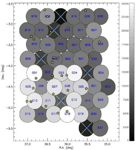
To date, the X-ray data received consist of a single region of roughly 6 $deg^{2}$ covered by 51 XMM-Newton pointings. Most of the observations (32 pointings, hereafter B pointings) were obtained through XMM AO1/AO2, and have a nominal exposure time of $10^{4}s$, whilst 19 (hereafter G pointings) are deeper $2\times 10^{4}s$ guaranteed time observations. The latter constitute the XMM Medium Deep Survey (XMDS, Chiappetti et al. 2005).

Figure 1: Sky distribution of the C1 clusters. The colour scale indicates the on-axis exposure time of each pointing in seconds (after particle flare filtering). Pointings marked by a cross are strongly affected by flares and will be re-observed during AO5.

Calibrated event lists were created using the XMM-SAS tasks emchain and epchain, and periods of intense proton flares were filtered out using the method suggested by Pratt & Arnaud (2002). Out of the 51 observations, 6 (including one G pointing) were too strongly contaminated to properly monitor and remove the high flare periods. These pointings are scheduled for re-observation during XMM AO5 and, consequently, are not included in the analysis of the present paper, which covers only 5 deg².

Details of the observations can be found in the publication of the full X-ray catalogue pertaining to this first 5 deg² (Pierre et al., submitted).

2.2 Data pre-analysis

For each pointing, images were generated in the [0.5-2] keV band from the filtered event lists using the XMM-SAS task evselect.

These were subsequently analyzed using the XMM-LSS source detection pipeline (described in detail by Pacaud et al. 2006): First, the images are filtered using a wavelet multi-resolution algorithm (Starck & Pierre,, 1998) that was specifically designed to properly account for the Poisson noise in order to smooth the background and lower the noise level, while keeping unchanged the relevant information. Then SExtractor is used on the filtered images to extract a very deep primary source catalogue. Finally, detailed properties of each detected source are assessed by Xamin, a maximum likelihood profile fitting algorithm that we have developed to characterize extended sources in XMM-Newton images.

2.3 Source selection process

2.3.1 Definition of the sample

As shown by Pacaud et al. (2006), the probability of detecting an extended source at the XMM-LSS sensitivity and resolution depends on both its flux and angular extent. This led us to abandon the simple concept of a flux limited cluster survey and to define a system of extended source classes: the final source selection is performed in the Xamin output parameter space, and several samples are defined, allowing for various amounts of contamination from point sources and spurious detections. The sub-samples, or classes, have been defined by means of extensive ‘in situ’ simulations, involving a large range of cluster fluxes and apparent sizes, for the nominal exposure of the XMM-LSS, i.e. $10^{4}s$. In this paper, we focus on the Class 1 sample (hereafter C1) which was defined from our simulations to be the largest uncontaminated extended source sample available. It is obtained by selecting candidates with extension $>$ 5″, extension likelihood $>$ 33, and detection likelihood $>$ 32. Given that no spurious extended detection was found in our whole simulated dataset, we are confident that the false detection rate is close to zero, and visual inspection of the X-ray/optical overlays for the C1 sources showed the existence of a cluster of galaxies or of a nearby galaxy as an optical counterpart in every case. Furthermore, we find that the C1 sample coincides with clusters for which a reliable temperature can be obtained using X-ray spectroscopy from the survey data (section 3.2).

Detailed information on the C1 selection process can be found in Pacaud et al. (2006).

2.3.2 Selection function

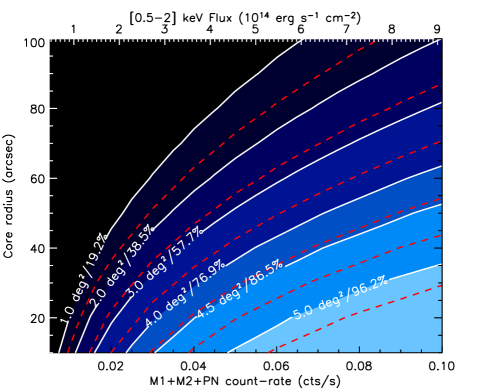
Given the varying effective exposure time per pointing, the survey coverage is not uniform ($7<t_{exp}/10^{3}s<20,$ Fig. 1). Consequently, similar likelihood values do not exactly pertain to the same objects across the survey. Rather than lowering all exposures to $7\times 10^{3}$s, we apply the C1 criteria to every pointing in order to maximize the size of the cluster sample. The probability of detecting a cluster of a given flux and extent for any pointing is subsequently derived by applying an analytic correction to the $10^{4}s$ simulations, scaling as a function of exposure time the S/N produced by such an object. This is justified by the fact that the range spanned by the exposure times is modest ($1/2<t_{exp}/10^{4}s<2$), implying also that source confusion does not change significantly. The survey selection function, i.e. the probability to detect a source of a given flux and apparent size as a C1 cluster, is obtained by integrating the contributions from all pointings. It is this function that is used in the following for cosmological applications. It is displayed in the form of a sky coverage in Fig. 2. The maximum area covered reaches 5.2 deg². This happens e.g. for sources with 20″core radius, and fluxes above $5\times 10^{-14}$ $\rm erg\,s^{-1}cm^{-2}$. Our sensitivity drops by roughly a factor of two for sources with flux around $1.5\times 10^{-14}$  $\rm erg\,s^{-1}cm^{-2}$ and $20\arcsec$ core radius, or $5\times 10^{-14}$ $\rm erg\,s^{-1}cm^{-2}$ flux and $75\arcsec$ core radius.

Figure 2: The survey coverage is displayed in a 2D parameter space: the sky coverage is a function of both cluster flux and extent. The dashed lines are the result of extensive 10ks simulations. The slightly shifted white lines are the analytical corrections accounting for exposure variations across the surveyed area, hence indicating the effective selection function of the current data set. The sample completeness corresponding to each line is indicated in terms of both the sky coverage and the percentage of detected sources. Extent values correspond to the core radius of a $\beta$-model with $\beta=2/3$. The count-rate to flux conversion assumes a 2 keV spectrum at $z=0$.

2.4 The sample

Applying the C1 selection criteria to the inner 11.5′of the 45 valid observations yields 37 detections, among which 4 are duplicated sources detected on adjacent pointings. Optical/X-ray overlays reveal that 5 of the remaining 33 sources are actually nearby X-ray emitting galaxies whose properties are presented in Appendix C. Hence we have a total of 28 galaxy clusters. An additional unambiguous C1 source is detected in pointing B13 (highly contaminated by flares); we provide the basic properties of this source in the present article, but it is not used in the scientific analysis as we cannot accurately compute the selection function for this pointing. The cluster sample is listed on Table 1. We note that a complementary cluster sample of about the same size has also been identified at lower significance in the same area; these clusters belong to our C2 and C3 classes, for which the selection criteria are much less well defined. They will be published in a separate paper (Adami et al., in prep.).

3 Assessing individual source properties

3.1 Spectroscopic validation

Each C1 X-ray source was confirmed as a bona-fide galaxy cluster at specific redshift via optical photometry and spectroscopy.

Table 1: List of the C1 galaxy clusters and their basic optical/X-ray properties. More information on peculiar individual clusters is provided in Appendix B.

Source name	XLSSC	Point.	R.A.	Dec.	Redshift	$N_{gal}$	$R_{spec}$	Counts	T	$R_{fit}$	Counts	FX in	r500	L500	$M_{500}$
	number		(J2000)	(J2000)			($\arcsec$)	in $R_{spec}$	($keV$)	(″/ Mpc)	in $R_{fit}$	0.5 Mpc	(Mpc)	($10^{43}$ $\rm erg\,s^{-1}$)	($10^{13}\,h^{-1}M_{\odot}$)
XLSS J022023.5-025027	039	B29	35.0983	-2.8409	0.23	3	66.5	144	$1.3^{+0.3}_{-0.1}$	54 / 0.198	112	$2.5^{+0.9}_{-0.9}$	0.417	$0.9^{+0.2}_{-0.3}$	$2.4$
XLSS J022045.4-032558	023	B26	35.1894	-3.4328	0.33	7	55.0	338	$1.7^{+0.3}_{-0.2}$	84 / 0.399	384	$4.4^{+0.4}_{-0.4}$	0.457	$3.8^{+0.3}_{-0.3}$	$3.1$
XLSS J022145.2-034617	006	B25	35.4385	-3.7715	0.43	26	80.0	1304	$4.8^{+0.6}_{-0.5}$	606 / 3.399	2099	$25.0^{+0.8}_{-0.7}$	0.838	$60.3^{+1.8}_{-1.8}$	$19$
XLSS J022205.5-043247	040	G09	35.5232	-4.5464	0.32	3	41.5	116	$1.6^{+1.1}_{-0.3}$	117 / 0.544	273	$2.1^{+0.3}_{-0.2}$	0.442	$1.6^{+0.2}_{-0.2}$	$3.4$
XLSS J022206.7-030314	036	B11	35.5280	-3.0539	0.49	3	46.5	507	$3.6^{+0.6}_{-0.4}$	213 / 1.286	659	$10.7^{+0.6}_{-0.5}$	0.676	$28.9^{+1.5}_{-1.5}$	$11$
XLSS J022210.7-024048	047	B28	35.5447	-2.6801	0.79	12	60.0	114	$3.9^{+2.8}_{-1.4}$	75 / 0.561	89	$1.6^{+0.3}_{-0.2}$	0.592	$13.2^{+2.2}_{-2.3}$	$12$
XLSS J022253.6-032828	048	B07	35.7234	-3.4745	1.00	3	55.0	137	$1.8^{+0.7}_{-0.4}$	66 / 0.529	94	$1.5^{+0.2}_{-0.2}$	0.327	$17.4^{+3.1}_{-3.1}$	$2.9$
XLSS J022348.1-025131	035	B16	35.9507	-2.8588	0.17	5	60.0	145	$1.2^{+0.1}_{-0.1}$	162 / 0.469	334	$4.8^{+0.5}_{-0.5}$	0.394	$0.77^{+0.07}_{-0.07}$	$1.5$
XLSS J022356.5-030558	028	B12	35.9857	-3.0997	0.30	8	60.0	144	$1.3^{+0.2}_{-0.2}$	60 / 0.267	118	$2.7^{+0.4}_{-0.4}$	0.399	$1.5^{+0.2}_{-0.2}$	$1.5$
XLSS J022357.4-043517	049	G08	35.9892	-4.5883	0.49	4	25.0	76	$2.2^{+0.9}_{-0.5}$	456 / 2.753	722	$1.9^{+0.2}_{-0.2}$	0.493	$4.3^{+0.4}_{-0.4}$	$3.4$
XLSS J022402.0-050525	018	G18	36.0087	-5.0904	0.32fn:willis	14	35.0	203	$2.0^{+0.7}_{-0.4}$	75 / 0.349	245	$1.5^{+0.2}_{-0.2}$	0.521	$1.3^{+0.2}_{-0.2}$	$4.7$
XLSS J022404.1-041330	029	G04	36.0172	-4.2251	1.05	5	33.5	310	$4.1^{+0.9}_{-0.7}$	60 / 0.486	355	$3.1^{+0.2}_{-0.2}$	0.524	$48.3^{+3.7}_{-3.4}$	$8.9$
XLSS J022433.8-041405	044	G03	36.1411	-4.2347	0.26fn:D1	10	54.5	319	$1.3^{+0.2}_{-0.1}$	294 / 1.183	544	$2.8^{+0.2}_{-0.2}$	0.399	$1.2^{+0.1}_{-0.1}$	$2.0$
XLSS J022456.2-050802	021	G17	36.2345	-5.1339	0.08	7	28.5	265	$0.68^{+0.04}_{-0.02}$	75 / 0.113	372	$3.3^{+0.6}_{-0.5}$	0.297	$0.11^{+0.01}_{-0.01}$	$0.9$
XLSS J022457.1-034856	001	B03	36.2381	-3.8157	0.61	23	60.0	730	$3.2^{+0.4}_{-0.3}$	129 / 0.869	770	$7.6^{+0.3}_{-0.4}$	0.584	$33.2^{+1.5}_{-1.5}$	$8.3$
XLSS J022520.8-034805	008	B03	36.3370	-3.8015	0.30fn:willis	11	45.0	99	$1.3^{+0.7}_{-0.2}$	57 / 0.254	104	$2.1^{+0.3}_{-0.3}$	0.396	$1.2^{+0.2}_{-0.2}$	$1.4$
XLSS J022524.7-044039	025	G07	36.3531	-4.6776	0.26fn:D1	15	35.0	661	$2.0^{+0.2}_{-0.2}$	153 / 0.615	925	$8.7^{+0.4}_{-0.4}$	0.533	$4.6^{+0.2}_{-0.2}$	$4.1$
XLSS J022530.6-041420	041	G02	36.3777	-4.2391	0.14fn:D1	15	45.0	523	$1.34^{+0.14}_{-0.06}$	159 / 0.392	785	$20.2^{+1.0}_{-1.1}$	0.440	$2.4^{+0.1}_{-0.1}$	$2.2$
XLSS J022532.2-035511	002	B03	36.3844	-3.9200	0.77fn:hz	11	37.5	225	$2.8^{+0.8}_{-0.5}$	66 / 0.489	200	$2.8^{+0.3}_{-0.3}$	0.493	$19.6^{+1.8}_{-1.8}$	$5.8$
XLSS J022540.6-031121	050	B13	36.4195	-3.1894	0.14	13	86.0	1386	$3.5^{+0.6}_{-0.5}$	177 / 0.436	1509	$48.2^{+2.2}_{-2.4}$	0.804	$9.3^{+0.5}_{-0.6}$	$16$
XLSS J022559.5-024935	051	B18	36.4982	-2.8265	0.28	11	60.0	224	$1.2^{+0.1}_{-0.1}$	57 / 0.242	169	$1.5^{+0.6}_{-0.3}$	0.384	$0.9^{+0.2}_{-0.1}$	$4.4$
XLSS J022609.9-045805	011	G11	36.5413	-4.9682	0.05fn:D1	9	67.5	424	$0.64^{+0.06}_{-0.04}$	465 / 0.454	1045	$11.6^{+1.1}_{-1.1}$	0.290	$0.11^{+0.01}_{-0.01}$	$0.6$
XLSS J022616.3-023957	052	B18	36.5681	-2.6660	0.06	2	46.5	529	$0.63^{+0.03}_{-0.03}$	102 / 0.118	802	$14.0^{+1.7}_{-1.4}$	0.285	$0.25^{+0.02}_{-0.02}$	$0.9$
XLSS J022709.2-041800	005	G01	36.7885	-4.3000	1.05fn:hz,fn:D1	9	35.0	164	$3.7^{+1.5}_{-1.0}$	96 / 0.777	179	$1.1^{+0.1}_{-0.1}$	0.489	$17.1^{+2.0}_{-2.0}$	$8.9$
XLSS J022722.4-032144	010	B10	36.8435	-3.3623	0.33fn:willis	9	60.0	452	$2.4^{+0.5}_{-0.4}$	96 / 0.456	440	$6.3^{+0.4}_{-0.4}$	0.574	$6.1^{+0.5}_{-0.5}$	$6.1$
XLSS J022726.0-043216	013	G05	36.8586	-4.5380	0.31fn:willis,fn:D1	18	30.0	160	$1.0^{+0.1}_{-0.1}$	417 / 1.899	536	$2.1^{+0.2}_{-0.2}$	0.340	$1.3^{+0.1}_{-0.1}$	$1.3$
XLSS J022738.3-031758	003	B15	36.9098	-3.2996	0.84fn:hz	13	48.0	231	$3.3^{+1.1}_{-0.7}$	393 / 2.998	523	$4.2^{+0.4}_{-0.4}$	0.518	$37.8^{+3.5}_{-3.3}$	$6.3$
XLSS J022739.9-045127	022	G10	36.9165	-4.8576	0.29fn:D1	9	39.5	1305	$1.7^{+0.1}_{-0.1}$	171 / 0.744	1791	$9.8^{+0.3}_{-0.3}$	0.471	$6.2^{+0.2}_{-0.2}$	$3.2$
XLSS J022803.4-045103	027	G10	37.0143	-4.8510	0.29	7	60.0	438	$2.8^{+0.6}_{-0.5}$	123 / 0.535	577	$6.1^{+0.4}_{-0.4}$	0.653	$4.8^{+0.4}_{-0.3}$	$9.1$

Table 2: Instrumental characteristics for each spectrograph configuration employed during the observations. All spectral observations were performed with a slit width of between 1$\aas@@fstack{\prime\prime}$0 and 1$\aas@@fstack{\prime\prime}$4.

Telescope	Instrument	$\rm Grism+Filter$	Wavelength	Pixel sampling	Spectral	Identifier
			interval (Å)	($\rm\AA\,{pix}^{-1}$)	resolution (Å)
VLT	FORS2	$\rm 300V+GG435$	4000–9000	3.2	14	1
VLT	FORS2	$\rm 600RI+GG435$	5000–8500	1.6	7	2
VLT	FORS2	$\rm 600z+OG590$	7500–10000	1.6	7	3
Magellan	LDSS2	medium–red	4000–9000	5.1	14	4
NTT	EMMI	Grism #3	4000–9000	3.0	8	5

The overall procedure used to confirm individual clusters is very similar to the approach taken in previously published XMM-LSS papers (Valtchanov et al. 2004; Willis et al. 2005; Pierre et al. 2006) and is summarised below.

A combination of either CTIO/MOSAIC II $Rz^{\prime}$ (Andreon et al., 2004) or CFHT/MEGACAM $ugriz$ imaging was used to associate the location of each X-ray source with the spatial barycentre of a significant overdensity of galaxies displaying characteristically red colours. Based on the CTIO data, galaxies lying within a given colour tolerance of this “red sequence” were then flagged as candidate cluster members and given a high priority in subsequent multi-object spectroscopic observations. A small number of low X-ray temperature ($\lesssim 1$ keV) groups at moderate redshift ($z>0.2$) and local ($z<0.2$) compact groups did not display a statistically significant red galaxy overdensity. These systems were inspected visually and spectroscopic targets were assigned manually.

Due to the moderately large size and the extended redshift range covered by the sample, cluster targets were observed using a number of facilities over several observing semesters. Details of the observing configurations can be found in Table 2.

Spectroscopic data were reduced using standard procedures described in detail in previously published XMM-LSS publications (Valtchanov et al. 2004; Willis et al. 2005; Pierre et al. 2006). Where possible, redshift values and associated uncertainties of individual galaxy targets were computed via cross-correlation with galaxy reference templates. In the remaining cases redshifts were assigned manually, from emission features.

The nominal condition adopted by XMM-LSS to confirm a cluster redshift is to observe three concordant redshifts (typically $\Delta z\lesssim 0.01$) within a projected scale of about 500 kpc of the cluster X-ray centre. Only cluster XLSSC-052 does not fulfill this condition: the X-ray emission is associated with a pair of $z=0.06$ galaxies very close to a bright star. Except for this specific system, the number of galaxy members confirmed per cluster ranges between 3 and 15, with a typical cross-correlation velocity error of order 50-150 km s^-1 per galaxy. Despite this velocity accuracy, we are limited for a large fraction of our sources by small-number statistics and consequently quote redshifts only to $\pm 0.01$. In each case, the final cluster redshift is computed from the unweighted mean of all galaxies lying within $\pm 3,000~{}\rm km.s^{-1}$ of the visually assigned redshift peak.

3.2 Spectral analysis

In order to measure the temperature of the intra-cluster gas, X-ray spectra were extracted in a circular aperture around each source. The corresponding background emission was estimated within a surrounding annulus having inner radius large enough for the cluster contribution to be considered negligible. Preliminary modelling of the cluster surface brightness profile allowed the determination of the optimal extraction radii in terms of S/N.

The resulting spectra were fitted using Xspec to a thermal plasma model (APEC) assuming a fixed hydrogen column density set to the Galactic value as derived from H I observations by Dickey & Lockman (1990). The metal abundance of the gas was held fixed during the fitting process at 0.3 times the solar abundance, as estimated by Grevesse & Sauval (1998). As explained in Willis et al. (2005), the cluster spectra were constructed imposing a minimum requirement of 5 background photons per bin in order to avoid the apparent bias we identified in Xspec temperature estimates when using the Cash statistic on very sparse spectra. Our simulations (Willis et al., 2005) showed that this procedure provides quite reliable temperature measurements ($\pm 10-20\%$) for $\sim$1-3 keV clusters having only a few hundred counts. We further investigated the impact of fixing the metal abundance at $0.3~{}Z_{\odot}$, by computing best fit temperatures obtained using extreme mean abundances of $0.1$ and $0.6~{}Z_{\odot}$. In most cases, the temperatures fell within the $1\sigma$ error bars from our initial fit. For five systems (namely XLSSC-008, XLSSC-028, XLSSC-041, XLSSC-044 and XLSSC-051) one of these two extreme measurements just fell a few percent outside of our error range. The measured temperatures are presented in Table 1.

3.3 Spatial analysis

3.3.1 Surface brightness modelling

To accurately determine the cluster fluxes and luminosities we modelled the observed photon spatial distribution in the [0.5-2] keV band with a radial $\beta$-profile:

$$S(r)=\frac{S_{0}}{[1+(r/R_{c})^{2}]^{3\beta-1/2}},$$ (1)

using a refined version of the method described in Pierre et al. (2006).

For each source, we started by fitting the mean background levels (vignetted and particle components) over the inner 13′ of the pointing, excluding all sources detected by the pipeline. Then, for each EPIC camera, the photons were binned within 3″ annuli centred on the cluster peak. The resulting profiles were subsequently rebinned imposing a minimum $S/N$ of 3 with respect to the estimated background level, weighted by the annular exposure times, and finally co-added to build a MOS1+MOS2+PN count-rate profile. The fitted model is constructed by convolving the circular $\beta$-profile with an analytical parametrization of the PSF (Ghizzardi et al., 2001), as implemented by Arnaud et al. (2002). The $\chi^{2}$ statistic is computed over a discrete grid of $\beta$ and $R_{c}$ values, with the value of the normalization coefficient, $S_{0}$, optimised analytically.

As already discussed in Pierre et al. (2006), the majority of the clusters are faint, and the detected photon distribution in many cases represents only a fraction of the extended X-ray surface brightness distribution. Under such conditions the parameters $\beta$ and $R_{c}$ are degenerate when fitted simultaneously, limiting the extent to which ‘best-fitting’ parameters can be viewed as a physically realistic measure of the cluster properties, although they provide a useful ad hoc parametrisation (Appendix 17). For this reason, we do not quote here best fitting values of $\beta$ and $R_{c}$ derived for each confirmed cluster. A dedicated analysis of the mean cluster profiles, obtained by stacking the data as a function of redshift and temperature, is underway (Alshino et al in prep.).

The photon count-rate within a specified radius is obtained by integrating the best-fitting spatial profile. The conversion into [0.5-2] keV flux and unabsorbed rest-frame bolometric ([0.001-50] keV) luminosity is performed via Xspec using the cluster temperatures previously derived.

3.3.2 Luminosity and flux determination

Luminosities are integrated within $r_{500}$ i.e. the radius at which the cluster mass density reaches 500 times the critical density of the Universe at the cluster redshift. As in Willis et al. (2005) and Pierre et al. (2006), this radius is estimated from the cluster mean temperature using the M-T relation of Finoguenov, Reiprich & Böhringer (2001), converted to ${\Lambda}CDM$ cosmology, which gives:

$$r_{500}=0.375~{}T^{0.63}~{}h_{73}(z)^{-1}~{}Mpc,$$ (2)

where T is expressed in keV and $h_{73}$ is the hubble constant in units 73 km s^-1Mpc^-1. Although “total” fluxes are often quoted in the cluster literature, our simulations show that the present data do not allow us to reliably perform such measurements (see Appendix 17). To limit extrapolation uncertainties, aperture flux values are computed by integrating within a fixed radius of 0.5 Mpc. As conspicuous in Table 1, 0.5 Mpc is generally smaller than $2\times R_{fit}$ except for the nearby low temperature groups XLSSC-039, XLSSC-021 and XLSSC-052. We chose to compute the flux within 0.5 Mpc (rather than $R_{500}$, which is generally smaller), since this is a similar approach to aperture photometry. For all clusters it corresponds to about 2/3 of the total flux, i.e. integrated to infinity, assuming a profile defined by $\beta=2/3,~{}R_{c}=180$ kpc. We emphasise that these fluxes are only used in the comparative analysis of the log(N)-log(S) relation, while $L_{500}$ and $M_{500}$ (along with $T$) are the actual physical quantities used in our cosmological modelling and in the subsequent discussion.

Finally, the $1\sigma$ errors on the extrapolated fluxes and luminosities are computed by identifying the region of the ($S_{0}$, $R_{c}$,$\beta$) parameter space where $\Delta\chi^{2}\leq 1$, and computing the extreme values of the extrapolated count-rates allowed by these models (see Appendix 17 for further discussion on the flux measurement accuracy).

3.3.3 Mass determination

Based on our best spatial fit profile, we estimate cluster masses, assuming that the gas is isothermal (the limited number of photons does not allow us to derive temperature profiles). Under these assumptions, for $M_{500}$ in $M_{\odot}$, the hydrostatic equilibrium assumption yields (see e.g. Ettori 2000):

$$M_{500}=1.11\,10^{14}\times\beta R_{c}T\frac{x_{500}^{3}}{1+x_{500}^{2}},$$ (3)

where $x_{500}=r_{500}/R_{c}$ (with $r_{500}$ given by Eq. 2), $R_{c}$ is expressed in Mpc, and $T$ in keV.

Values of $r_{500}$, flux and luminosity for the C1 clusters are listed in Table 1, together with $M_{500}$.

Figure 3: Redshift distribution of the C1 sample. The colour scale indicates the cluster mean temperature for each bin (unweighed mean of the individual cluster temperatures in keV) .

4 Results

4.1 Global properties of the sample

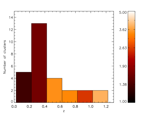
The detected clusters span the [0.05-1.05] redshift range with a pronounced peak around $z\sim 0.3$ (Fig. 3). Roughly half of the objects have a temperature lower than 2 keV, pointing to a large fraction of groups in our sample. As a natural consequence of its sensitivity, good PSF and dedicated source detection procedure, the XMM-LSS systematically unveils for the first time the $z\sim 0.3$, $T\lesssim 2$ keV cluster population on large scales. We note also that none of the objects detected so far exhibits strong lensing features. In the following, we will generally use the word “cluster” regardless of the temperature, while “group” specifically refers to objects below 2 keV. A noticeable feature of the sample, illustrated by Fig. 3, is the increasing mean cluster temperature with redshift. Given the strong correlation between X-ray luminosity and temperature (Sec. 4.3) this can readily be understood as the unavoidable Malmquist bias. Moreover, the current sky coverage of the survey makes the sample likely to be affected by cosmic variance. Both issues will be given special attention in the following cosmological analysis.

Additional information on individual sources, including possible contamination by AGN emission, are discussed in Appendix B. We also display the optical images of each cluster with confirmed member galaxies and X-ray contours overlayed.

4.2 The $M_{500}$-$L_{X}$ relation

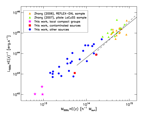
The correlation between cluster luminosities and masses derived from the spatial analysis is shown in Fig. 4. Once self-similar evolution is assumed, our data points appear to be continuous with the massive cluster samples of Zhang et al. (2006) and Zhang et al. (2007) [respectively at $z\sim 0.3$ and $z\sim 0.2$]. Moreover, the scatter in the relation is relatively low (i.e. almost comparable to that of the high mass sample). This overall consistency is remarkable in the sense that, for half of the clusters, less than 500/300 photons were available for the spatial/spectral fitting. This provides an important indicator of the reliability of our measurements, and could be further interpreted as adding weight to the self-similar evolution hypothesis.

The comparison between our data points and the indicative $M$-$L_{X}$ relation derived from Arnaud, Pointecouteau & Pratt (2005) and Arnaud & Evrard (1999) also suggests some flattening of the correlation at the low mass end. Our luminosity sampling, however, suffers significant Malmquist bias, and masses derived from a single isothermal $\beta$-model fitting are known to be underestimated (Vikhlinin et al, 2006). Both effects tend to contribute to the apparent flattening in the $M$-$L_{X}$ relation.

4.3 The $L_{X}$-$T$ relation

The correlation between the observed luminosity and the temperature of our clusters is shown in Fig. 5. The comparison with the local relation measured by Arnaud & Evrard (1999) suggests a positive redshift evolution of the luminosity at a given temperature. To test this, we performed an analysis of the enhancement factor, $F(z,T)=L_{X}/L_{X}(T,z=0)$, with respect to this local reference. In most of the intra-cluster gas models, $F$ is a simple function of redshift: the self-similar assumption yields $F(z)=E(z)$ where $E(z)=H(z)/H_{0}$, is the evolution of the Hubble constant. More elaborate models that include non-gravitational physics (i.e. cooling and heating) generally propose an evolution of the form $F(z)=(1+z)^{\alpha}$ (e.g. Voit 2005). All these models assume that the entire cluster population follows a unique evolutionary track. In the present study, we adopted this hypothesis, since the Malmquist bias prevents us from investigating the extent to which evolution could be a function of cluster temperature.

Figure 4: The Mass-Luminosity relation for the sample clusters. Because of the large redshift range spanned by the data, the mass and luminosity parameters are scaled assuming self-similar evolution (factor $E(z)$, see Sec. 4.3). For comparison, the massive cluster samples from Zhang et al. (2006) and Zhang et al. (2007) are also shown. The dashed and solid lines also show the mean $M_{500}$-$L_{X}$ relation infered from the $M_{500}$-$T$ and $L_{X}$-$T$ measured in Arnaud, Pointecouteau & Pratt (2005) and Arnaud & Evrard (1999) respectively for $T>$ 3.5 keV and $T>$ 2 keV.

Table 3: Trends in the literature for the modelling of F(z) as a power law of $(1+z)$. For comparison, constraints from the C1 sample were added, ignoring the selection effects.

Ref.	power of (1+z)
Vikhlinin et al. (2002)	$1.5\pm 0.3$
Novicki, Sornig, & Henry (2002)	$2.1\pm 1.1$
Ettori et al. (2004)	$0.6\pm 0.3$
Lumb et al. (2004)	$1.5\pm 0.3$
Kotov & Vikhlinin (2005)	$1.8\pm 0.3$
Maughan et al. (2006)	$0.8\pm 0.4$
C1 clusters with $0.1<z<0.4$ (14 sources)	$2.3\pm 0.8$
C1 clusters with $0.4<z<1.1$ (10 sources)	$1.3\pm 0.5$
All C1 clusters above $z=0.1$ (24 sources)	$1.5\pm 0.4$

To date, various attempts to constrain $F(z)$ as a power law in $(1+z)$ have yielded discordant results (see Table 3). Several explanations for this discrepancy have been invoked: poor statistics, deviations between the several available local reference relations, disparity in mass and redshift of the current high-z cluster samples (if $F$ is not a simple function of $z$), as well as biased samples. Although limited by photon statistics, the XMM-LSS cluster sample, with its well controlled selection function, provides an important opportunity to test the impact of the selection process in such studies.

In a preliminary analysis, Willis et al. (2005) measured a mean value $F=1.46$ from an initial XMM-LSS sample covering the $[0.30-0.43]$ redshift range. Another estimate using the D1 subsample (Pierre et al. 2006, section 3.4) also found a luminosity enhancement for the $z\sim 0.3$ domain, and showed that it could be statistically significant only above $T\sim 1.5$ keV. However, none of these studies fully addressed the impact of selection biases on the derived results.

Figure 5: The $L_{500}$-$T$ relation. Same symbols as in Fig. 4. The sources that are used for the analysis of the $L_{X}-T$ evolution (circles) have redshifts in the range [0.14-1.05] and fall on average above the local $L_{X}$-T relation of Arnaud & Evrard (1999) (shown by the solid line).

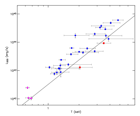
In the present article, involving a larger sample, we perform a self-consistent likelihood analysis of our data parameter space, for a given $F(z)$. We excluded from the analysis XLSSC-050 (contaminated by flares), XLSSC-018 (contaminated by an AGN), and the 3 local groups ($z\lesssim 0.1$ and $T\lesssim 1$ keV) for which our measurements could be affected by a large radial extrapolation and by X-ray emission from member galaxies. The available sample for this analysis is thus restricted to 24 objects.

4.3.1 The likelihood model

Figure 6: Comparison of the modelled $L_{X}$-T distribution with and without selection effects for several redshifts, assuming self-similar evolution. The light and dark shaded regions show, for each temperature, the luminosity interval than contains respectively 95.5 and 68.3% of the expected detections. The solid line gives the maximum of the luminosity PDF for each temperature; it is cut at the temperature for which the detection probability (integrated over $L_{X}$) falls to 5%. For comparison, the local Arnaud & Evrard (1999) relation, evolved according to the self-similar model, is indicated by the short dash line, and the 1 and 2$\sigma$ bounds arising from our scatter model are shown by dotted lines. The long dash line is the local relation.

Folding our selection function into the analysis of the $L_{X}-T$ relation cannot be achieved by the usual $\chi^{2}$ fitting. Instead, we have to estimate the likelihood of our data, given a $F(z)$ model. We thus start by assuming that cluster luminosities are distributed by a log-normal probability density function (PDF) around the mean value $L_{mean}(T,z)=L(T,z=0)\times{F(z)}$, which we will call the true distribution:

$$\frac{dP_{true}(L_{X}|T,z)}{d\ln{L_{X}}}=\frac{1}{\sqrt{2\pi}\sigma_{\ln{L_{X}}|T}}\exp{\left(-\frac{\ln{\left(L_{X}/L_{mean}\right)}^{2}}{2\sigma_{\ln{L_{X}}|T}^{2}}\right)}.$$ (4)

An estimate of the scatter in the local $L_{X}$-T relation is provided by Stanek et al. (2006). The authors fitted a single dispersion value to the Reiprich & Böhringer (2002) sample (thus assuming that it is the same from the group regime to large clusters) and obtained $\sigma_{\ln{T}|L_{X}}=0.25$. We further assume that this scatter does not evolve with redshift. Combining the lognormal distribution with the power law shape of the mean $L_{X}-T$ relation, we get $\sigma_{\ln{L_{X}}|T}\sim 2.7\times 0.25\sim 0.7$ where 2.7 is the approximate $L_{X}-T$ slope in the Reiprich & Böhringer (2002) sample.

The normalised PDF for detection of a cluster with such $L_{X}$ and $T$ is then the product of the ‘true’ PDF with our selection function:

$$\frac{dP_{det}(L_{X}|T,z)}{d\ln{L_{X}}}=P_{0}(T,z)\times\frac{dP_{true}(L_{X}|T,z)}{d\ln{L_{X}}}\times f(L_{X},T,z),$$ (5)

where:

$$P_{0}(T,z)=\left(\int\left[\frac{dP_{true}(L_{X}|T,z)}{d\ln{L_{X}}}\times f(L_{X},T,z)\right]\ d\left(\ln{L_{X}}\right)\right)^{-1}.$$ (6)

We compute $f(L_{X},T,z)$ (from Fig 2), assuming a canonical value of 180 kpc for the cluster core radii. The resulting modification of the PDF is illustrated in Fig. 6 at different redshifts assuming self-similar evolution: including selection effects in the likelihood model renders underluminous cool clusters undetectable. Note that for clusters with temperatures close to the detection threshold at any given redshift, the bias in mean $L_{X}$ at a given $T$ due to selection effects can be a factor 2 or more.

Figure 7: Evolution of the $L_{X}$-$T$ relation. (a): Raw analysis. The data points from several studies are plotted (stacked into redshift bins for clarity). Whenever possible, we converted luminosity estimates from the other samples to $L_{500}$ using the information provided by the authors. The following differences remain: the luminosities of the Lumb et al. (2004) clusters are estimated within the virial radius; the data points of Maughan et al. (2006) also include the clusters from Vikhlinin et al. (2002) and have luminosities estimated within $R_{200}$. Overlaid are several enhancement factor fits from our baseline analysis: the (1+z) power law and ad-hoc 2 parameter fits to our data alone (resp. short and long dashed lines), and the (1+z) power law and ad-hoc 2 parameter fits (resp. dot-dashed and 3dot-dashed lines) fitted to the C1 clusters combined with the samples of Kotov & Vikhlinin (2005) and Ettori et al. (2004). For comparison, the self-similar prediction is indicated by the solid line. (b): Taking into account selection effects. The filled circles and short dashed line recalls the location of our raw data points, and best fit model from the preliminary analysis. The corrected enhancement factor fit for the 2 parameter model is shown as the long dashed line. The final 1 parameter fit and its $1\sigma$ confidence interval is displayed by the solid line and the shaded region. Expectations from several intra-cluster gas models are plotted for comparison: the self-similar predictions (dotted line) and two models by Voit (2005) including non gravitational physics (dot-dashed and 3dot-dashed lines)

Practically, errors on the luminosity can be considered as negligible, since the fractional errors on temperature are usually much larger and the $L_{X}-T$ relation goes like $T^{3}$. The likelihood of an observed cluster C being drawn from a given $F(z)$ is thus obtained by marginalizing over the possible cluster temperatures, i.e.:

$$L(F|C)=\int_{0}^{+\infty}\left[\frac{dP_{det}(L_{X}|T,z)}{d\ln{L_{X}}}\right]\times P_{C}(T)dT,$$ (7)

where $P_{C}(T)$, the temperature PDF of the cluster, is derived from the C-statistic distribution provided by the Xspec’s steppar command. Finally, the likelihood of the enhancement factor is computed as the product of the detection probabilities, for the given F(z), of all clusters pertaining to our sample:

$$L(F)=\prod_{i=0}^{N}L(F|C_{i})$$ (8)

To estimate errors on fitted parameters, we identify $-2\ln{L(F)}$ with a $\chi^{2}$ distribution, as is asymptotically valid in the limit of large samples according to Wilks’ theorem, and quote 68% confidence intervals. The same identification is used to assess how much a given model deviates from the best fit $F(z)$ by correcting the measured $\Delta\chi^{2}$ to the equivalent value that yields the same probability for 1 free parameter.

4.3.2 Raw fit

In a first step, we neglect the selection function in our formalism (i.e. effectively imposing $f(L_{X},T,z)=1$ in the likelihood computation). This will both provide us with a reference point to assess the impact of the selection process, and allow for comparison with previous work, where the issue of sample selection has been ignored.

As shown in Table 3, fitting the usual $F(z)=(1+z)^{\alpha}$ yields $\alpha=1.5\pm 0.4$, which is consistent with Vikhlinin et al. (2002), Lumb et al. (2004) and Kotov & Vikhlinin (2005). Nevertheless, this simple model does not seem to correctly reproduce the observations over the full redshift range: the values of $\alpha$ obtained over $[z=0.1-0.4]$ and $[z=0.4-1.1]$ are incompatible at the one sigma level (see Table 3). Interestingly, Ettori et al. (2004) noticed a similar discrepancy within their own sample, but did not consider its implications for their subsequent analysis.

In Fig. 7a, we display simultaneously our data points along with those from previous studies. Error bars are large, but the points suggest a non-monotonic evolution, with a maximum around $z\sim 0.5$, thus excluding an enhancement factor of the form $F(z)=(1+z)^{\alpha}$. This may explain the diverging results of Table 3. Consequently, we fitted an ad hoc two-parameter model of the form $F(z)=(1+z)^{\alpha}\times E(z)^{\beta}$. This model is intrinsically degenerate and would need very accurate data to individually constrain $\alpha$ and $\beta$, but has the ability to reproduce the apparent non-monotonic evolution. Since cases $\alpha=0$, $\beta=1$, and $\beta=0$ correspond to the self-similar and power law models respectively, we may evaluate through this parametrization how much the observations deviate from any of them.

A fit over the C1 clusters yields $\alpha=4.7$ and $\beta=-5.4$ and excludes the self-similar evolution at the $3.5\sigma$ level. Our best $(1+z)^{\alpha}$ model is however less than $0.4\sigma$ away from the best fit and the evidence of a non-monotonic evolution is thus rather weak from our data alone (the probability of such a deviation being real is roughly 45%). This is not the case any longer when including also in the fit the data from Kotov & Vikhlinin (2005) and Ettori et al. (2004), for which we could convert the luminosity to $L_{500}$. A simple power law model is then ruled out at the $8.4\sigma$ level based on 59 sources.

4.3.3 Taking into account selection effects

With this comparison baseline, we can now turn to investigate the impact of our selection process on the observed $L_{X}$ enhancement (restoring the correct value of $f(L_{X},T,z)$ in the likelihood). This task is tractable here because the XMM-LSS C1 selection function has been thoroughly assessed.

Maximizing the likelihood over our ad hoc two-parameter model now yields $\alpha=1.3$ and $\beta=-1.3$. As can be seen in Fig. 7b, the inferred evolution rate is considerably lower than with the raw fit. As a result, the self-similar expectation is now less than $7\times 10^{-2}\sigma$ away from the best fit model, and the statistical evidence for a non-monotonic evolution is virtually null. To evaluate the remaining deviation from self-similarity, we switch back to a one parameter model by fixing $\beta=1$. The best fit value for $\alpha$ is then $-0.07^{+0.41}_{-0.55}$, and the corresponding $F(z)$ is shown in Fig. 7b.

This latter analysis points to a negative evolution of the $L_{X}$-T relation (i.e. $L(z|T)$ increases with $z$) over the $0<z<1$ range. These results quantitatively favour the self-similar hypothesis, although our current data set is still marginally consistent with no evolution at all as is clear from Fig. 7b.

This is illustrated in more detail in Fig. 8 for the $z\sim 0.3$ intermediate redshift, where the 1-2 keV groups make up the peak of the XMM-LSS sensitivity (cf. section 5).

Figure 8: Similar to figure 6 for $z=0.3$, with the $0.2<z<0.4$, with C1 clusters overlaid. Again, the dashed line is the evolved model of Arnaud & Evrard (1999). The triangles indicate the D1 clusters presented by Pierre et al. (2006). The only cluster (XLSSC-018, square) that falls well below the Arnaud & Evrard (1999) $L_{X}$-T relation, and at the limit of our $2\sigma$ contour, is likely to be contaminated by an AGN (see Appendix B).

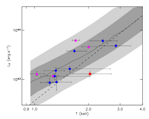
These results are still preliminary because of the poor statistics (in both the number of sources and the temperature estimates). Moreover, they are likely to be very sensitive to the choice of the local $L_{X}$-$T$ reference (including scatter) due to the redshift-temperature correlation within the sample. Nevertheless, our findings seriously question any attempt to assess the evolution of cluster scaling laws without modelling the full source selection process.

In the rest of the article, we assume that the cluster scaling laws evolve following the self-similar model, as suggested by the above analysis.

5 COSMOLOGICAL MODELLING

In this section, we compare the observed properties of the C1 sample with cosmological expectations based on the latest WMAP constraints (Spergel et al., 2006).

5.1 The model

We model the cluster population and its evolution following Pacaud et al. (2006), but with slightly modified assumptions as to the cluster scaling laws.

The linear power spectrum $P(k)$ of dark matter fluctuations is computed using an initial power law of index $k^{n_{s}}$ and the transfer function from Bardeen et al. (1986), taking into account the shape parameter:

$$\Gamma=\Omega_{m}h\times exp\left[-\Omega_{b}\left(1+\sqrt{2h}/\Omega_{m}\right)\right]$$ (9)

introduced by Sugiyama (1995). The overall power spectrum is normalised at z=0 to $\sigma_{8}$, and the redshift evolution is obtained from the linear growth factor (Carroll, Press, & Turner, 1992). Based on this power spectrum, we use the Jenkins et al. (2001) formalism to derive the dark matter halo mass function $dn/dm(z)$. This procedure is an accurate fitting of the mass function obtained from numerical simulations, provided one defines the mass of the halo to be that included inside $r_{200b}$, the radius enclosing an overdensity of 200 with respect to the mean background density.

In order to reproduce the C1 selection function, we need to translate the mass parameter into observable parameters, which is practically achieved by means of scaling laws. Usually, halo masses in such relations are defined with respect to the critical density of the Universe (and not to the background density). Hence, the need to assume a model for the halo profiles to connect the two mass definitions. For this purpose, we used NFW profiles (Navarro, Frenk & White, 1997) with a scaling radius $r_{s}$ provided by the model of Bullock et al. (2001) which relates $r_{s}$ to the virial mass of the halo through the concentration parameter $c=r_{vir}/r_{s}$. The $M_{500}-M_{vir}$ conversion was obtained from the formulae provided in the Appendix C of Hu & Kravtsov (2003), with the estimate of the overdensity within the virial radius from Kitayama & Suto (1996).

The gas temperature within the dark matter halos is then computed using the $M_{500}$-$T$ relation of Arnaud, Pointecouteau & Pratt (2005), i.e. a power low of slope $\alpha=1.49$, valid for clusters with $T>4$ keV. To account for the steepening of the relation at lower temperatures suggested by their data, we used a higher slope of $\alpha=1.9$ below 3 keV. The lower halo mass limit is then fixed by imposing $T~{}>~{}0.5$ keV. Bolometric luminosities are derived using the $L_{X}$-$T$ relation of Arnaud & Evrard (1999). Self-similar evolution is assumed for both these scaling laws.

To account for the scatter observed in cluster properties, we encapsulate the dispersion of the M-T and L-T relations in the M-L relation, for the sake of simplicity. We assign the X-ray luminosity assuming a log-normal distribution. Following Stanek et al. (2006), who measured $\sigma_{ln{M}|L}=0.37$, we use $\sigma_{ln{L}|M}\sim 0.37\times 1.59\sim 0.6$ where 1.59 is the slope of their $M-L_{X}$ relation. The total XMM-NEWTON EPIC count rate is estimated using the same spectral model as in section 3.2, with a fixed hydrogen column density of $2.6\times 10^{20}$ cm^-2 (representative of our field), folded through the EPIC response matrices for the THIN filter in accordance with our observing mode. The selection function (Fig. 2) is finally applied assuming, as in the previous section, a constant physical core radius of $180$ kpc.

In what follows, given the still modest size of the current cluster sample (some 30 objects over 5 deg²) we restrict most of the comparisons to qualitative visual ones.

5.2 The redshift distribution

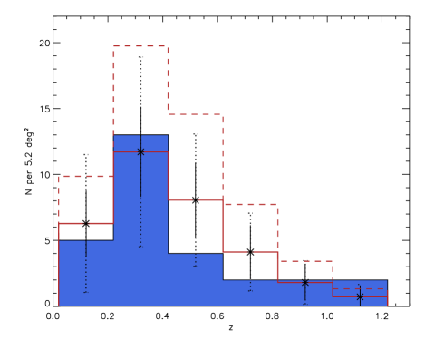
Our model (using $\sigma_{8}$ = 0.74, from WMAP3) predicts $6.2$ Class 1 clusters per square degree which, assuming Poisson noise alone (i.e.$\pm 1.1$ for the current 5.2 ), is compatible with our observed density of $5.4$ deg^-2 as given by the objects listed in Table 1.

The observed redshift distribution of the C1 sources, shown in Fig. 9, shows good overall agreement with the model expectations, and suggests that we are crossing a void-like region within $0.4<z<0.6$. As is evident from the errors in Fig. 9, this apparent underdensity can be fully accounted for by statistical plus cosmic variance. We estimated the cosmic variance using the formalism from Hu & Kravtsov (2003), under the assumption that the surveyed volume is enclosed within a top-hat sphere; in the sensitivity regime of the XMM-LSS survey, the total uncertainty on the $N(z)$ bins scales roughly as $2\sqrt{N}$.

Interestingly, the C1 cluster density predicted assuming $\sigma_{8}=0.85$ (as inferred by Spergel et al. 2003 from the $1^{st}$ year WMAP data) is 14.6 deg^-2 and appears to be much higher than required to match our observations. In this case, even using a non-evolving $L_{X}-T$, which is roughly our $1\sigma$ lower bound from the previous section, our model predicts 10.7 C1 clusters per deg². Our data are 3.7$\sigma$ (considering Poisson fluctuations) below this latter model. Even including cosmic variance, the difference is approximately 2$\sigma$. This suggests that increasing the area by a factor of 2 would already permit a stringent test of the value of $\sigma_{8}$ indicated by WMAP.

In this context, we examine in detail in Sec.6.3 some parameters which play a role in the interpretation of the cluster number counts.

Figure 9: Redshift distribution of the C1 sample. The filled histogram shows the redshift distribution of our sample, while the solid line shows the expectations of our cosmological model (WMAP3: $\sigma_{8}=0.74$ and self-similar evolution for the $L_{X}-T$ relation). Expected fluctuations around the mean model density due to shot noise and (shot noise + cosmic variance) are respectively displayed with the solid and dotted error bars. The dashed line shows the expectations for a model with WMAP $1^{st}$ year cosmological parameters ($\sigma_{8}=0.85$) and a non-evolving $L_{X}-T$ relation; combining this latter $\sigma_{8}$ value with self-similar evolution would produce a normalisation even higher, by about 35%.

5.3 The Flux and luminosity distribution

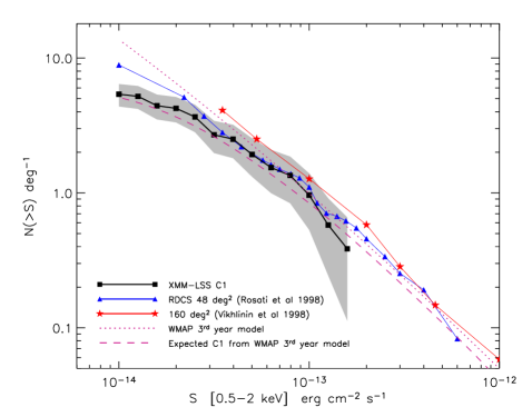
As our selection function does not depend on flux alone, as assumed in previous generations of surveys, we have no direct estimate of the log(N)-log(S) relation. In this section, we provide the necessary information to enable the inter-comparison between our statistical distributions and those of past as well as future surveys.

Our cosmological model can be both compared to the local log(N)-log(S), and used to predict an expected distribution for our C1 sample . This is shown in Fig. 10. The raw log(N)-log(S) from our model is first compared with the estimates from Rosati et al. (1998) and Vikhlinin et al. (1998) based on flux limited samples, and said to be corrected for selection effects as well as for incompleteness. We find overall consistency, although our model suggests a somewhat higher total cluster density than the RDCS measurements above a flux of $\sim 10^{-14}$  $\rm erg\,s^{-1}cm^{-2}$. Furthermore, the predicted flux distribution, once folded with the C1 selection function, is consistent within the errors with the C1 log(N)-log(S) relation derived from the present sample. This adds credibility to our full selection process and log(N)-log(S) modelling.

Figure 10: The C1 log(N)-log(S). The squares show the observed C1 number counts and the shaded region indicates the $1\sigma$ error region. Overlaid are the predictions from our model: the dashed line for C1 clusters, and the dotted line for the whole cluster population (i.e. all clusters above a given flux). Since only a fraction of cluster fluxes are detected in any survey, there is an important caveat in this comparison: our model delivers total cluster fluxes (i.e integrated to infinity) while our measurements are performed within $0.5~{}$Mpc (which includes $\sim 2/3$ of the total flux for a cluster with $R_{c}=180$ kpc and $\beta=2/3$). Previously, Vikhlinin et al. (1998) claimed to measure total fluxes in an unbiased manner, while Rosati et al. (1998) estimated that they had recovered at least 80-90% of the total flux.

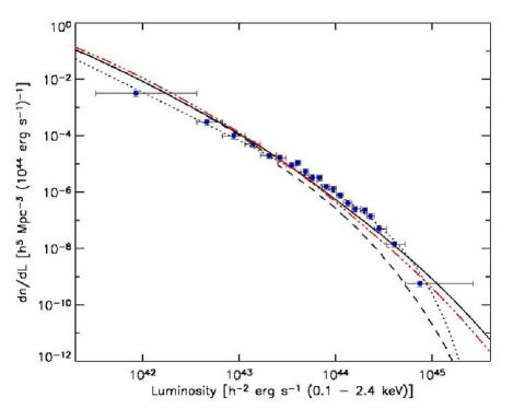
Similarly, our sample is currently too small to derive the cluster luminosity function at any redshift, but this again can be predicted by our model. We first compute as a cross-check the local luminosity function and compare it with the estimates from the REFLEX survey (Böhringer et al. 2002), which constitutes the largest complete cluster sample currently available at low-redshift (Fig. 11). The model shows, on average, good agreement with the measured REFLEX luminosity function (which accounts for the survey sky coverage). It lies slightly below the REFLEX measurements for luminosities in the range $5\times 10^{43}$-$5\times 10^{44}$ $\rm erg\,s^{-1}$, behavior that is also present in the ROSAT Bright Cluster Sample (Ebeling et al, 2000) as can be appreciated in the comparative plots of Mullis et al. (2004). We further emphasize that, as is conspicuous in Fig. 11, the inclusion in the model of scatter in the $M-L_{X}$ relation is necessary in order to obtain predictions that are compatible with the REFLEX constraints at the high $L_{X}$ end. Finally, we note that the prediction of our model at $z=0.8$ (also displayed in Fig. 11) is very similar to the local one out to $L_{X}=10^{44}$ $\rm erg\,s^{-1}$, and about a factor of 2 lower at $L_{X}=10^{45}$ $\rm erg\,s^{-1}$ (although still within the REFLEX error bars). Since the EMSS (Gioia et al, 1990), the question of the evolution of the cluster luminosity function has been controversial, especially for luminosities above $5\times 10^{44}$ $\rm erg\,s^{-1}$ [see a review by Mullis et al. (2004) including several ROSAT samples]. The most recent determination of the cluster luminosity function for $L_{X}<10^{44}$ $\rm erg\,s^{-1}$ from the COSMOS-XMM data shows no evolution (Finoguenov et al., 2007). Our calculations suggest that, interestingly, for a concordance cosmology, the observed luminosity function does not significantly evolve out to $z\sim 0.8forL_{X}<10^{44}$ $\rm erg\,s^{-1}$, while the cluster mass-function and scaling laws do. This can be regarded as a ‘conspiracy’ between cosmology and cluster physics.

5.4 Mass-observable relations

Last but not least, our model provides us with a tool for deriving heuristic mass-observable relations. For this purpose, we adopt the very general parametrisation introduced by Hu (2003):

$$OBS\ =\ OBS_{0}\left(\frac{M_{d}}{M_{0}}\right)^{p(z)}\times e^{A(z)},$$ (10)

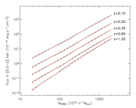
where $M_{d}$ is the mass defined within some overdensity $d$, $OBS$ is the observable of interest (flux, count-rate) and $M_{0}$ and $OBS_{0}$ are reference values for both quantities. In practice, we used $M_{0}=10^{12}~{}h^{-1}M_{\odot}$ and $M_{d}=M_{200b}$ i.e. the mass enclosed within the radius delineating an overdensity of 200 with respect to the mean background density. Model data points for a large range of masses, redshifts and fluxes (count-rates) were fitted with the above formula as illustrated on Fig. 12. We found that the functions $p(z)$ and $A(z)$ are sufficiently well described by functionals of the form:

$$\left\{\begin{array}[]{l}p(z)=p_{0}+p_{1}\,z\\ A(z)=a_{0}\,z^{a_{1}}.\\ \end{array}\right.$$ (11)

Table 4: Parameters of the mass-observable calibration from our cosmological model, as defined by equations 10 and 11.

Parameter	mass-flux relation	mass$\,-\,$count-rate relation
$OBS_{0}$	$0.0329$	$1.23\times 10^{10}$
$a_{0}$	$-37.68$	$-36.50$
$a_{1}$	$0.0645$	$0.0680$
$p_{0}$	$1.45$	$1.41$
$p_{1}$	$0.248$	$0.269$

The best fit values for the Mass vs Count-rate and Mass vs Flux relations are provided in Table 4. We do not give errors on the parameters as the overall accuracy of both fits with respect to the model data is better than 15% over the $0.05<z<1.2$ and $2\times 10^{13}<M<2\times 10^{15}~{}h^{-1}M_{\odot}$ ranges. In practice, the intrinsic dispersion of the M-L relation also needs taking into account. Assuming $\sigma_{ln{L}|M}\sim 0.6$ (Sec. 5.1) this translates into a dispersion of -45% +82% in the Flux$-$ or Count-rate$\,-\,$Mass relation. Thus “perfect” flux measurements may yield, via this formula, mass accuracies of the order of -60% +100%. Such an empirical relation has obvious useful practical usages. It should be noted however, that extrapolating the formulae in the current form above $z>1.2$ is not straightforward as a number of prominent low temperature lines ($O_{VII},~{}Fe_{VII},~{}Fe_{VIII}$) are redshifted below the 0.5 keV boundary, creating discontinuities that cannot be accounted for with the above simple functionals.

Figure 11: The local luminosity function predicted by our model, compared with the REFLEX data points (Böhringer et al., 2002). The dotted line is the best fit to the REFLEX data from the original article. The dashed line is the expectation from our model assuming no scatter in the $M-L_{X}$ relation. The solid line shows our model (including scatter) yielding a much better agreement. The 3dot-dashed line is the prediction of our model for a redshift of 0.8.

.

Figure 12: Calibration of the [0.5-2] keV band total flux vs $M_{200b}$ relation. The exact correlations derived from our model are shown for several redshifts with plain lines. The overplotted dashed lines show the recovered values using the fit presented in Table 4.

6 Discussion

We have shown that an accurate understanding of the sample selection effects is essential for a proper study of the evolution of the L-T relation of clusters of galaxies. Once these are allowed for, our data are compatible with self-similar evolution but cannot exclude no evolution at all. Subsequently, we have defined a cosmological cluster evolutionary model to which we applied the survey selection function. It matches well our observations in terms of cluster number density, redshift and flux distribution, hence providing a theoretical basis to further explore the ability of large XMM cluster surveys to constrain cosmology.

In this respect, one of the critical issues is the role and the number of cluster parameters involved in the cluster scaling law evolution. As a first step, we have shown that for our best fitting model, it is possible to derive good mass-observable relations for the entire population of interest. We realistically explore below the impact of various parameters and hypotheses on the cluster scaling laws, on the selection function and, subsequently, on cluster number counts. In this way we hope to pave the way for future investigations.

6.1 Cluster shape parameters

Our selection function, as applied to our model, assumes a fixed core radius of $R_{c}=180$ kpc. Since $R_{c}$ is related to the overall physical size of the system, one naturally expects this value to depend on the cluster mass (or on any related parameter). This should ideally be included in the cosmological analysis, but we are currently lacking a well established $R_{c}-T$ relation. The slope reported by Ota & Mitsuda (2004) is, for instance, much stronger than the one observed in the Sanderson & Ponman (2003) sample. Ota & Mitsuda (2002) also revealed that, due to cool cores, the core radius distribution infered by performing a single $\beta$-model analysis over the whole cluster population is actually double peaked and thus ill-defined.

Furthermore, another known observational feature of X-ray groups and clusters is the tendency of the $\beta$ parameter to drop with decreasing system temperature (see e.g. Jones & Forman 1999, or more recently Osmond & Ponman 2004) but this correlation remains poorly defined, specially in the group regime. As our selection function is mainly surface brightness limited, we expect the detection probability to depend on $\beta$ as well as $R_{c}$ and so, two additional scaling relations are needed.

One could in principle derive them from the observed sample, but, given the generally small number of collected photons, it is not possible to resolve precisely the $\beta-R_{c}$ degeneracy for most of our sources. Furthermore, such a study would be complicated by the fact that our selection process is dependent on these parameters, thus requiring a sophisticated self-consistent modelling similar to what was done in Section 4.3 for the $L_{x}-T$ relation.

Given the small number of systems in the present sample, we postpone such a study to a future paper investigating the evolution of mean cluster/group profiles by stacking images (Alshino et al in prep.)

6.2 The evolution of the $L_{X}-T$ relation

The constraints we were able to put on the evolution of the L-T relation ($\alpha=-0.07^{+0.41}_{-0.55}$ for the $F(z)=E(z)\times(1+z)^{\alpha}$ model) are not only limited by the relatively modest size of the sample and the uncertainties on the temperature measurements, but also depend on the assumed scatter of the relation (this parameter was fixed in the fit).

6.2.1 Impact of the assumed scatter value

In order to quantify the impact of the scatter in the determination of the evolution of the L-T relation, we ran a series of fits assigning different values to $\sigma_{\ln{L}|T}$. We find that the $\alpha$ index describing the deviation from self-similarity can be modelled by the following empirical formula:

$$\alpha=1.78-\left(\frac{\sigma_{\ln{L}|T}}{0.45}\right)^{1.41}.$$ (12)

The uncertainty on $\sigma_{\ln{T}|L}$ of $\sim 25\%$ quoted by Stanek et al. (2006) along with the $L_{X}-T$ slope uncertainty (say between 2.5 and 3) yield an uncertainty of $\sim 20\%$ for $\sigma_{\ln{L}|T}$ (same reasoning as in Sec. 4.3.1). This translates to a conservative confidence range of $[0.5-0.9]$ for $\sigma_{\ln{L}|T}$, which in turn gives fitted values of $\alpha$ in the range $[0.6,-0.87]$. The corresponding deviation is thus larger than the statistical errors from our fit, and precise constraints on $\sigma_{\ln{L}|T}$ are definitely required in order to place firm and rigorous constraints on $F(z)$. Given that the scatter in the $L_{X}-T$ relation could well be a function of redshift and mass, one will have to wait for large samples of high-z clusters with well monitored selection effects in order to undertake a fully self-consistent determination of the evolution of the slope and scatter of the $L_{X}-T$ relation.

6.2.2 Impact of the sample size and of the uncertainties on the temperature

We have further investigated the extent to which the determination of the slope of the evolution of the $L_{X}-T$ relation is conditioned by the size of the cluster sample and by the magnitude of the error bars on the temperature (in comparison, errors on the luminosity are assumed to be negligible). We have thus simulated a large number of random cluster catalogues corresponding to 5, 20, and 64  XMM-LSS type surveys. The realisations are drawn from our cosmological model, reproducing our observed $n(z,T)$ distribution along with selection effects; self-similarity is assumed for the $L_{X}-T$ evolution. Each cluster temperature is assigned a mean error estimated from the spectral fitting simulations presented in the appendix of Willis et al. (2005), for 10 ks XMM exposures. In addition, we have considered the possibility of dedicated deep XMM follow-up observations providing a temperature accuracy of 10% for cluster subsamples of various sizes. For each sample, the slope was fitted following the method described in Sec 4.3.1 and 4.3.3. Results are summarized in Table 5.

Table 5: Expected accuracy in the determination of the evolution of the $L_{X}-T(z)\propto E(z)(1+z)^{\alpha}$ relation for various sizes of XMM-LSS type surveys, estimated from simulations. The temperature measurements come either directly from the 10 ks XMM exposures, with corresponding accuracy. Or, part of them are improved by subsequent deep XMM observations, assuming an uncertainty of 10%; the last column gives the number of such clusters to undergo deep XMM pointings. $\sigma_{\alpha}$ is the mean 1$\sigma$ error on $\alpha$ for a survey realisation.

Area	Temperature accuracy	$\sigma_{\alpha}$	$N_{re-obs}$
5	from the survey	0.59	-
20	” ”	0.28	-
64	” ”	0.15	-
5	10% for the $z>0.8$ clusters	0.58	2
20	” ”	0.25	14
64	” ”	0.14	41
5	10% for the $z>0.5$ clusters	0.50	9
20	” ”	0.22	45
64	” ”	0.13	139

The simulations show that a significant improvement can be reached by increasing the sample size as the accuracy on $\alpha$ scales roughly as the square root of the surveyed area. This is a very noticeable result, given that 2/3 of our clusters have no more than 500 counts available for the spectral fit. The spectral accuracy is of the order of 20% below 2 keV, and 50% around 5 keV (Willis et al., 2005), the latter concerning mostly distant clusters. The simulations further show that increasing the accuracy of the temperature measurements does not yield a very significant improvement on the slope of the $L_{X}-T$ relation - compared to the amount of time that would be necessary to obtain accurate temperatures for the $0.5<z<1$ hot clusters. This is mostly due to the fact that the dispersion in the $L_{X}-T$ relation itself is large. Quantitatively, applying the $\sqrt{area}$ rule of thumb on Fig. 7b, shows that a 10  area (or any sample with a similar size and controlled selection effects) has the potential to exclude the non evolution hypothesis. But even with 600 clusters (i.e. a 64  area, and 140 very well measured clusters above $z>0.5$) it seems difficult to, for example, discriminate between the two modified-entropy models of cluster evolution proposed by Voit (2005).

6.2.3 Working on samples close to the detection limit

Fig. 8 shows that for the $0.2<z<0.4$ range, most of our clusters are detected in a $L_{X}-T$ region where the selection effects are significant, as is to be expected, given that lower mass halos are much more numerous than massive ones. As a result, overluminous clusters will be overrepresented in our sample. For the present data set, this is also true at any redshift, and this situation is easily understandable as a result of the combined effects of (1) the high efficiency of Xamin close to the detection limit (it was designed to enable the construction of the largest possible controlled cluster sample), and (2) the steepness of the cluster mass function. Generally speaking, given the contradictory former results obtained from data based on heterogeneous ROSAT-selected samples, our findings suggest that graphs such as Fig. 8 should be first carefully constructed, when studying the cluster $L_{X}-T$ relation at any redshift.

6.3 Modelling the cluster number density

While most of the ingredients linking cosmology to the expected cluster distribution are rather well established (mass functions, mean scaling relations for massive clusters) many details of the mass-observable issues are still pending. Among these, we would cite : the evolution of cluster scaling laws, the scaling laws in the group regime, and the role of the scatter in all relations. Our analysis has shown that our current data are compatible with self-similar evolution for the L-T relation. In this section we thus focus on two other specific aspects, namely the slope of the M-T relation for the groups and the scatter in the M-L relation. We illustrate below the sensitivity of the cluster number counts to these quantities by means of our model.

6.3.1 The M-T relation in the group regime

Figure 13: Impact of the steepening of the $M-T$ relation in the group regime on the modelling of the cluster number density. The full line corresponds to our fiducial model (broken power law, Sec. 5.1), giving 6.2 clusters per deg². If we assume the Vikhlinin et al (2006) result (single slope of 1.5, dash line), the cluster density drops to 3.6 deg^-2. The relation of Arnaud, Pointecouteau & Pratt (2005), motivated by a possible steepening of the mass function below 3.5 keV, (single slope of 1.7, dash-dot line) seems to be closer to our observations and yields a cluster density of 6.9 deg^-2.

Our model assumes that the $M-T$ relation for both massive clusters and groups can be modelled by a broken power law. Recent measurements [Vikhlinin et al (2006) and Arnaud, Pointecouteau & Pratt (2005)] agree very well in the high mass regime, but yield contradictory results for groups. Vikhlinin et al (2006) claimed that the previously reported steepening of the relation (by e.g. Finoguenov, Reiprich & Böhringer 2001) resulted from a bias toward low mass, due to an incorrect modelling of the density profile at large radius. However, their assertion relied on only two low-temperature systems. On the other hand, Arnaud, Pointecouteau & Pratt (2005) found a steepening at low temperature based on a larger sample of groups, but their analysis assumes a NFW profile at large radius. As this point is currently still controversial, we adopted an intermediate solution: a steepening to 1.9 of the relation below 3 keV (note that a change in the $L_{X}-T$ relation for groups would have similar impact). Fig. 13 illustrates how the various hypotheses on the shape of the $M-T$ relation in the low-mass regime impact on the cluster number counts. Our assumed broken power-law model provides the best fit on the basis of visual inspection, but the difference to the Arnaud, Pointecouteau & Pratt (2005) model is not statistically significant with the current sample size.

6.3.2 Impact of the scatter

Figure 14: Impact of scatter in the $M-L_{X}$ relation on the predicted C1 redshift distribution. For given scatter values, the predicted total number of clusters per deg² are respectively : 3.6 (no scatter), 5.1 (0.3), 8.4 (0.9); our model gives 6.2 (0.6) .

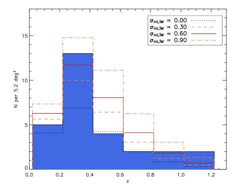
We discussed above how the scatter in the $L_{X}-T$ relation influences the determination of the evolution of the relation from the observations (Sec. 6.2.1) . In our model, all sources of dispersion are encapsulated in the $M-L_{X}$ relation, since the determination and understanding of dispersion in $L_{X}-T$ and $M-T$, and thus $M-L_{X}$, and of their possible evolution, is still in its infancy. In this respect, we note that measurements of scatter other than those of Stanek et al. (2006) are available: lower values for $\sigma_{\ln{L}|M}$ have been found by Zhang et al. 2006 and Zhang et al. 2007 (respectively 0.41 and 0.33), but they are dominated by higher temperature systems which are known to have more regular properties. In terms of the accuracy with which the scatter is determined, the typical errors estimated by Stanek et al. (2006) lead to an uncertainty in $\sigma_{\ln{L}|M}$ of the order of 20%.

In Fig. 14, we show the impact on the C1 redshift distribution of neglecting the scatter in $M-L_{X}$, as well as the influence of plausible values of scatter. If the luminosities are symmetrically scattered around the expected value for a given mass, the net effect on our cluster counts (approximately the number of clusters detected above a given luminosity at a given redshift) is an increase of the detected cluster density since, due to the steepness of the mass function, substantially more low-mass clusters become detectable than high-mass cluster undetectable.

6.4 Cosmology and cluster survey self-calibration

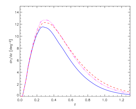
We have demonstrated that taking into account survey selection effects is not only critical for the proper modelling of the cluster number counts (hence cosmology) but also for the determination of the cluster evolutionary scaling laws, which in turn, also impact on $dn/dz$ (Fig. 9). Further, we explored the impact on $dn/dz$ of the slope of the $M-T$ relation (Fig. 13) and of the dispersion in the scaling laws (Fig. 14). This illuminated, by means of real data, the magnitude of some of the degeneracies between cosmology and cluster evolution. However, the number of cosmological free parameters that we have explored in the present study is very limited (basically, only $\sigma_{8}$, Fig. 9) and a more general analysis should, among others, include constraints on the Dark Energy parameter $w$. For instance, in Fig. 15 we exhibit the predictions of our model for different values of $w$ and $\alpha$ (evolution parameter of $L_{X}-T$). A clear degeneracy is apparent, adding to those already reviewed.

In order to cope with this critical issue, it has been suggested that X-ray (or SZ) cluster number counts, in principle, have the ability to self-calibrate even an evolving mass-observable relation, because the number density of clusters as a function of redshift has a fixed functional form given by cosmological simulations (Levine, Schulz & White 2002; Hu 2003; Majumdar & Mohr 2003). This suggests the possibility of simultaneously solving for the cosmology and fitting an ad hoc parametrized mass-observable relation, provided that a sample of several thousands of clusters is available.

While our - still somewhat phenomenological - best fitting model, allowed us to derive flux$-$ and count-rate$\,-\,$mass relations, several caveats still have to be pointed out. We have noticed that the flux-mass relation is very sensitive to the details of the X-ray emitting plasma (e.g. emission lines) and also, obviously, to the way fluxes are estimated in shallow XMM exposures; in earlier studies, even the temperature-dependence of the bremsstrahlung continuum was ignored (e.g. Majumdar & Mohr 2003). Even neglecting measurement uncertainties, our mass$\,-\,$observable mapping exhibit $1\sigma$ uncertainties in the range [-60%,+100%] coming solely from the dispersion of the $M-L_{X}$ relation.

In this respect, while vastly increasing the number of clusters may be useful, additional independent observations on cluster evolutionary physics will constitute a crucial input. This will improve the modelling of the mass-observable relations, and thus the constraints on the mass function. In particular, deeper XMM pointings will provide accurate temperatures and, consequently, a better estimate of the dispersion in the L-T relation. Weak-lensing, using the CFHTLS images, will provide independent mass measurements (Berge et al in prep.).

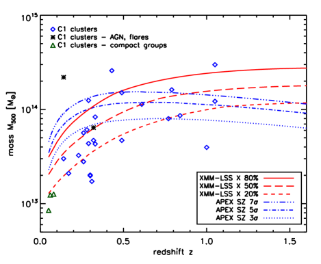
In the future, the XMM-LSS field will be covered by Sunyaev-Zel’dovich (SZ) observations [OCRA (One Centimeter Receiver Array), AMiBA (Array for MIcrowave Background Anisotropy) and APEX (Atacama Pathfinder EXperiment)]. Since the SZ decrement is an integral of the cluster pressure ($n_{e}T_{e}$) along the line of sight, and is independent of $z$, it provides an especially interesting complement to the X-ray emissivity (scaling as $n_{e}^{2}T_{e}^{1/2}$ for moderately hot clusters). Comparing our limiting mass as a function of redshift with those of these SZ surveys is all the more informative as we introduced a new class-oriented selection to define the XMM-LSS cluster sample. This is done, as a test case, in Fig. 16 for the XMM-LSS and the APEX-SZ surveys [Schwan et al. (2003), Dobbs et al. (2006)]. The SZ limit has been obtained under the assumption that APEX will observe at two frequencies (150 and 220 GHz) with a 1′ beam and 10 $\mu$K/beam white noise in each channel. We have included the effect of contamination by primary Cosmic Microwave Background (CMB) anisotropies. Given the spatial spectrum of the CMB, the instrumental noise and cluster profiles, we compute the expected SZ flux limit as a function of cluster size using matched filters. We then convert from SZ fluxes and sizes to masses and redshifts, using the same cosmology and scaling laws as in our X-ray modelling. Details of the computation are given in Melin et al. (2005).

The XMM-LSS mass limit of $10^{14}~{}M_{\odot}$ around $z=1$ for the C1 selection, appears comparable to the prediction for the deepest SZ surveys to date. In addition, the XMM-LSS uncovers more low-mass systems below $z<0.5$. According to our current model, the APEX-SZ cluster density detected at 3$\sigma$ is 3.8 deg^-2 out to $z=1$, to be compared with 5.4 deg^-2 for the observed C1 X-ray selection. In a forthcoming paper (Melin et al in prep.) we explore the cosmological constraints expected from a few hundred clusters, whose masses are determined by a joint X-ray/SZ/weak-lensing analysis.

Figure 15: Dark energy vs scaling laws for our modelled cluster reshift distribution. The solid line shows the prediction for the Spergel et al. (2006) cosmology and self-similar evolution of the scaling laws. Assuming instead $F(z)=E(z)\times(1+z)^{0.34}$ for the $L_{X}$-T evolution, which is our $1\sigma$ higher bound from section 4.3, yields the dotted-dashed line. As a comparison, the dashed line shows the distribution obtained by keeping self-similar evolution but changing the dark energy equation of state from -1 to -0.6.

Figure 16: Comparison of the XMM-LSS and APEX-SZ sensitivity in terms of limiting mass. The red lines show various probability detection thresholds for the C1 clusters. The blue lines are the predictions for the $10\mu K$ APEX survey (see text). The X-ray and SZ curves make use of the best fitting model to our current data set (Sec. 5.1).

7 SUMMARY AND CONCLUSION

• This work presents a well-controlled XMM cluster sample over 5 deg² with a density of 5.4 deg^-2 at medium X-ray sensitivity (down to $\sim 10^{-14}$  $\rm erg\,s^{-1}cm^{-2}$ for the extended sources in question). A complementary sample of about the same size, but with less well defined selection criteria is in preparation (Adami et al). We provide positions, redshifts, fluxes, luminosities, temperatures and masses along with X-ray and optical images.

• The selection is based on well-defined criteria pertaining to spatial extent properties, and are similar to a surface brightness (rather than flux) limit.

• The resulting cluster redshift distribution extends out to $z=1.2$ and peaks at $z\sim 0.3$. Half of the clusters have temperatures in the range 1-2 keV, occupying the $0.2<z<0.4$ interval. This intermediate population, the building blocks of the present day clusters, is systematically unveiled by the XMM-LSS survey. It is also the first time that a wide-area blind X-ray survey has provided reliable cluster temperature measurements.

• We demonstrate that taking into account the sample selection effects is vital for a proper determination of the evolution of the $L_{X}-T$ relation. This is due in large part to the steepness of the cluster mass function, which results in sources clustering close to the detection limit, and of these the overluminous systems are preferentially detected. This may explain the often contradictory results obtained with heterogeneous samples selected form ROSAT surveys.

• Modelling the selection effects carefully, our data appear to point to approximately self-similar evolution. A sample twice as large should allow exclusion of the no-evolution hypothesis, at better than the 1$\sigma$ level. Using extensive simulations, we find that increasing the sample size is more efficient than increasing the accuracy of the temperature measurements for constraining the evolution; this is due to the large intrinsic dispersion of the $L_{X}-T$ relation.

• Our results suggest a higher normalisation of the cluster log(N)-log(S) at faint fluxes than previously obtained by deep ROSAT surveys.

• Cluster masses were estimated from surface brightness profile fitting, assuming hydrostatic equilibrium. Our sample follows surprisingly well (given the very modest XMM exposures of $\sim$ 10 ks and our rudimentary modelling of the mass profile) the local $L_{X}-M$ relation, when evolved self-similarly.

• Self-consistent cosmological modelling of the cluster population, convolved with the accurately determined survey selection function, confirms that the properties of our current data set are compatible with the concordance cosmology along with cluster self-similar evolution.

• This model then allowed us to investigate several degeneracies arising from cluster physics, regarding the cosmological interpretation of the number counts. In particular, we stress the influence of the, still poorly determined, scatter in the cluster scaling laws.

• The present study led us to investigate many of the issues raised when attempting to perform precision cosmology using real cluster data, including the need for precise selection effects and a realistic error budget. Thanks to the temperature information obtained from the detected photons for all C1 clusters, this work constitutes one of the first attempts to break, in a self-consistent way, the degeneracy between cosmology and cluster evolution, in the analysis of the cluster number counts. The next step will be to apply cosmological modelling to the full XMM-LSS area ($10~{}deg^{2}$ - to be completed in 2007) adding input from the combined weak lensing and SZ survey as well as from the 3-dimensional cluster distribution.

• All data presented in this paper - cluster images taken at X-ray and optical wavebands in addition to detailed results for the spectral and spatial analyses - are available in electronic form at the XMM-LSS cluster online database: http://l3sdb.in2p3.fr:8080/l3sdb/.

Appendix A Notes on spatial fitting and photometric accuracy

Figure 17: Photometric accuracy of our spatial fitting procedure using simulations. The data points show the mean deviation from the true value in our simulation as a function of available signal (number of counts within spectral fitting radius $R_{fit}$), and the extrapolation factor (flux measurement within $R_{fit}$, $R_{fit}/2$, and $2*R_{fit}$). The solid error bars with short hats show the dispersion among measured values, while the dotted error bars with large hats gives the mean value of the $1\sigma$ bounds estimated by the procedure.

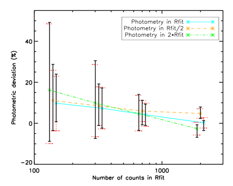
In this appendix, we test the accuracy of our luminosity measurement procedure, running the spatial fitting algorithm on simulated images.

For this purpose, we created $10^{4}s$ XMM pointing simulations with vignetted and particle background levels set to the mean observed values of Read & Ponman (2003), and point sources distributed according to the log(N)-log(S) of Moretti et al. (2003). We then randomly included in these simulations extended sources with $\beta=2/3$ and several $R_{c}$ and count rate values (respectively from 10 to 50″and 0.005 to 0.1 $\rm cts\,s^{-1}$). A $\beta$-profile was fitted to all the simulated sources that were detected by the first pass of our pipeline (see Pacaud et al. 2006 for details) and for which the spatial fitting procedure detects at least three radial bins above $3\sigma$.

The simulations showed that that below 400 detected counts in the spatial fitting radius, the degeneracy between $\beta$ and $R_{C}$ is large, but that the integrated flux (within the fitting radius) is well modelled by the best fitting ($\beta$,$R_{C}$) combination. Results of the simulations are presented in Fig. 17.

The measurements are almost unbiased: less than a few percent in general, and up to $\sim 10\%$ for very faint sources (100-200 counts). This small offset can be interpreted as a weak Eddington bias, as it is of the order of Poisson fluctuations, and probably results from our requirement of recovering at least 3 significant bins (which means retaining only the clusters that appear brighter among the faintest ones). This shouldn’t be an issue for the C1 clusters as they are generally brighter (see Table 1). The scatter around the mean value is very low for bright sources and mildly increases (up to $\sim 15\%$) for the faintest ones. Estimating the luminosity within a different radius than the fitting one does not result in significant differences (although the scatter increases) as long as the profile is not extrapolated too far out, which is the case for our sample. Finally, the mean estimated errors are of the same order as the dispersion of the best fit value, assessing our confidence intervals.

Other sources of error have already been considered by Pierre et al. (2006) appendix A: the impact of neglecting the errors on the temperature (which affects our estimate of $R_{500}$) was shown to be smaller than a few percent, while the contribution from undetected weak AGNs is probably lower than the percent level (which is comforted by the present simulations in which AGNs are included).

We thus conclude that the possible systematics generated with our fitting procedure are rather low, especially compared to the statistical errors.

Appendix B Individual characteristics of the C1 galaxy clusters

Figure 18: Gaussian smoothed X-ray emission from source XLSSC-018 at z=0.32 in bands [0.5-2] keV (left) and [2-10] keV (right). The emission in the soft band seems slightly offset from the cluster cD galaxy. In the hard band, the offset becomes much larger.

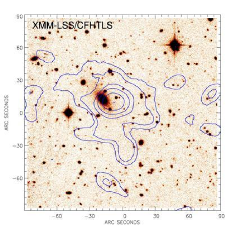
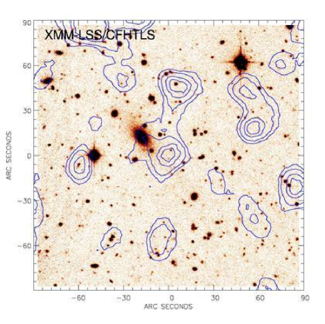
Notes on individual sources:

• XLSSC-028:
  The velocity information obtained to date on this object does not allow us to firmly conclude on its redshift. The two bright galaxies on which the X-ray emission is centred have a redshift of 0.08; their spectra are typical of elliptical galaxies, without emission lines. No other galaxies with this redshift have been measured in the field, but a number of z=0.3 objects are found within 500 kpc of the X-ray centroid. The measured X-ray temperature is 1.5 keV for z=0.3 and, the luminosity is found to be $1.6e43$ $\rm erg\,s^{-1}$, which puts the object close to the observed $L_{X}$-T relation. At z = 0.08, the source is about a factor of 17 fainter, and corresponds to a temperature of 0.75 keV which put it also exactly on the $L_{X}$-T relation.

• XLSSC-018:
  The first measurement of temperature of this system ($\sim 2.7_{-0.9}^{+2.5}$ keV, published in Willis et al. (2005)) was one of the hottest in our sample at a redshift around 0.3. Yet, the cluster doesn’t seem massive, neither in the X-ray nor in the optical. The emission in the [2-10] keV appears to be significantly displaced from the low energy centroid (Fig. 18), and is possibly associated with an optical counterpart. This suggests that a fraction of the emission could be due to an AGN. Excluding the probable contaminated region from the spectral fit lowers by a factor of two the number of available photons, but surprisingly leads to much tighter error bars around a temperature of $2.0$ keV (as reported in Table1). We regard this as strong evidence that the cluster’s X-ray emission suffers AGN contamination, and consequently discard this source from the $L_{X}-T$ analysis.

• XLSSC-006:
  This source was already studied in Willis et al. (2005), and assigned a luminosity of $(4.5\pm 0.3)\times 10^{44}$ $\rm erg\,s^{-1}$ which is incompatible with our estimated $(6.0\pm 0.2)\times 10^{44}$ $\rm erg\,s^{-1}$. In that paper, the luminosity was derived from the Xspec spectral fitting measurement, to which a correction factor was applied in order to extrapolate to $r_{500}$. We interpret the discrepancy as resulting from the combination of two effects. Firstly, Xspec uses a background estimate comming from an annulus surrounding the source, while in our spatial fitting procedures, we model it over the whole pointing. As a consequence, the mean background level used within Xspec actually happened to be higher than our fitted value due to residual contamination of the bright XLSSC-006 cluster in this local annulus. Additionaly, the observed source count-rate in the [0.5-2] keV band (on which our spatial fitting luminosity estimate is based), is found to be higher within Xspec than the one infered from the best spectral fitting model.
  

Information on other C1 sample clusters is already published by Valtchanov et al. (2004), Willis et al. (2005) and Pierre et al. (2006).

Appendix C The C1 nearby galaxies

These sources were discarded from the C1 galaxy cluster sample based on an obvious link between the main X-ray emission, and the presence of a nearby galaxy on the same line-of-sight. A significant fraction of the total X-ray emission can however originate from another object in the field. The source list is given in Table 6, and details regarding the origin of the X-ray emission are given below:

Table 6: The nearby galaxy sample. XMM pointing identifiers refer to the XMM-LSS internal naming convention as described in Pierre et al. (submitted); the location of each pointing on the sky is shown in figure 1.

Source name	Pointing	R.A.	Dec.
		(J2000)	(J2000)
XLSS J022528.7-040041	B03	36.3699	-4.0115
XLSS J022251.4-031151	B11	35.7146	-3.1975
XLSS J022659.2-043529	G06	36.7469	-4.5916
XLSS J022430.4-043617	G08	36.1268	-4.6048
XLSS J022617.6-050443	G16	36.5735	-5.0788

• XLSS J022528.7-040041:
  The nearby galaxy lying a the centre of the X-ray isophotes is alreday known as APMUKS(BJ) B022258.83-041412.5. The X-ray emission from this galaxy certainly originates from its interaction with two satellite companions, as conspicious in the images of Fig. 35.

• XLSS J022251.4-031151:
  This source is likely to result from the confusion of a point source with the nearby elliptical galaxy APMUKS(BJ) B022018.98-032531.1. It is associated with a radio source detected in Tasse et al. (2006).

• XLSS J022659.2-043529:
  The nearby galaxy lying at the centre of the X-ray isophotes is already known as MCG -01-07-011. We cannot exclude it to be the dominant galaxy of a poor nearby group, as its aspect is reminiscent of the compact group XSLC-011 at z 0.05.

• XLSS J022430.4-043617:
  This source is likely to result from the confusion of a point source with a nearby spiral galaxy. The galaxy is already known as 6dF J0224300-043614, and has a redshift of z=0.06916.

• XLSS J022617.6-050443:
  The nearby galaxy lying a the centre of the X-ray isophotes (APMUKS(BJ) B022347.26-051811.5) is detected as a weak radio source in Tasse et al. (2006). As for, XLSS J022659.2-043529, we cannot exclude the possibilty that it is the dominant galaxy of a small group. Another option would be that it is part of the recently identified XBONG class (see e.g. Yuan & Narayan 2004).

Figure 20: Images of the C1 clusters (sorted by right ascension). Left: X-ray/I band overlay of the central 7′. Right: true colour image with X ray contours and measured redshift in the central 1.5 Mpc. (a): XLSSC-039. (b): XLSSC-023.

Figure 21: continued

Images of the C1 clusters. (a) XLSSC-006. (b): XLSSC-040.

Figure 22: continued

Images of the C1 clusters. (a) XLSSC-036. (b): XLSSC-047.

Figure 23: continued

Images of the C1 clusters. (a) XLSSC-048. (b): XLSSC-035.

Figure 24: continued

Images of the C1 clusters. (a) XLSSC-028. (b): XLSSC-049.

Figure 25: continued

Images of the C1 clusters. (a) XLSSC-018. (b): XLSSC-029.

Figure 26: continued

Images of the C1 clusters. (a) XLSSC-044. (b): XLSSC-021.

Figure 27: continued

Images of the C1 clusters. (a) XLSSC-001. (b): XLSSC-008.

Figure 28: continued

Images of the C1 clusters. (a) XLSSC-025. (b): XLSSC-041.

Figure 29: continued

Images of the C1 clusters. (a) XLSSC-002. (b): XLSSC-050.

Figure 30: continued

Images of the C1 clusters. (a) XLSSC-051. (b): XLSSC-011.

Figure 31: continued

Images of the C1 clusters. (a) XLSSC-052. (b): XLSSC-005.

Figure 32: continued

Images of the C1 clusters. (a) XLSSC-010. (b): XLSSC-013.

Figure 33: continued

Images of the C1 clusters. (a) XLSSC-003. (b): XLSSC-022.

Figure 34: continued

Images of the C1 clusters: XLSSC-027.

Figure 35: Images of the C1 nearby galaxies: source XLSS J022528.7-040041. Left: 7′wide I band image overlayed with X-ray contours. Right: 5′wide true color image (g,r,i) overlayed with X-ray contours.

Figure 36: continued

Images of the C1 nearby galaxies. (a) XLSS J022251.4-031151. (b): XLSS J022659.2-043529.

Figure 37: continued

Images of the C1 nearby galaxies. (a) XLSS J022430.4-043617. (b): XLSS J022617.6-050443.

References

- Andreon et al. (2004) Andreon, S., Willis, J., Quintana, H., Valtchanov, I., Pierre, M., & Pacaud, F. 2004, MNRAS, 353, 353
- Arnaud & Evrard (1999) Arnaud, M., & Evrard, A. E. 1999, MNRAS, 305, 631
- Arnaud et al. (2002) Arnaud, M., Majerowicz, S., Lumb, D. et al. 2002, A&A, 390, 27
- Arnaud (2005a) Arnaud, M., 2005, astro-ph/0508159
- Arnaud, Pointecouteau & Pratt (2005) Arnaud, M., Pointecouteau, E., & Pratt, G. W. 2005, A&A, 441, 893
- Bardeen et al. (1986) Bardeen, J. M., Bond, J. R., Kaiser, N., & Szalay, A. S. 1986, ApJ, 304, 15
- Barkhouse et al. (2006) Barkhouse, W. A., et al. 2006, ApJ, 645, 955
- Böhringer et al. (2002) Böhringer, H., Collins, C. A., Guzzo, L. et al. 2002, ApJ, 566, 93
- Bremer et al. (2006) Bremer, M., Valtchanov, I., Willis, J. et al. 2006, MNRAS, 371, 1427
- Bullock et al. (2001) Bullock, J. S., Kolatt, T. S., Sigad, Y., Somerville, R. S., Kravtsov, A. V., Klypin, A. A., Primack, J. R., & Dekel, A. 2001, MNRAS, 321, 559
- Carroll, Press, & Turner (1992) Carroll, S. M., Press, W. H., & Turner, E. L. 1992, ARA&A, 30, 499
- Chiappetti et al. (2005) Chiappetti, L., Tajer, M., Trinchieri, G. et al. 2005, A&A, 439, 413
- Dickey & Lockman (1990) Dickey, J. M., & Lockman, F. J. 1990, ARA&A, 28, 215
- Dobbs et al. (2006) Dobbs, M., et al. 2006, New Astronomy Review, 50, 960
- Dupke & Bregman (2006) Dupke, R. A., & Bregman, J. N. 2006, ApJ, 639, 781
- Ebeling et al (2000) Ebeling, H.; Edge, A. C.; Allen, S. W.; Crawford, C. S.; Fabian, A. C.; Huchra, J. P., 2000, MNRAS, 318, 333
- Eke, Navarro & Steinmetz (2001) Eke, V. R., Navarro, J. F., & Steinmetz, M. 2001, ApJ, 554, 114
- Ettori (2000) Ettori, S. 2000, MNRAS, 311,313
- Ettori et al. (2004) Ettori, S., Tozzi, P., Borgani, S., & Rosati, P. 2004, A&A, 417, 13
- Finoguenov et al. (2007) Finoguenov et al. 2007, astro-ph/0612360
- Finoguenov, Reiprich & Böhringer (2001) Finoguenov, A., Reiprich, T. H., & Böhringer, H. 2001, A&A, 368, 749
- Ghizzardi et al. (2001) Ghizzardi, S. 2001, EPIC-MCT-TN-011 (XMM-SOC-CAL-TN-0022)202020 http://xmm.vilspa.esa.es/docs/documents/CAL-T-0022-1-0.ps.gz
- Gioia et al (1990) Gioia, I. M., Henry, J. P., Maccacaro, T., Morris, S. L., Stocke, J. T., Wolter, A. 1990, ApJ 356L, 35
- Grevesse & Sauval (1998) Grevesse, N., & Sauval, A. J. 1998, Space Science Reviews, 85, 161
- Jenkins et al. (2001) Jenkins, A., Frenk, C. S., White, S. D. M., Colberg, J. M., Cole, S., Evrard, A. E., Couchman, H. M. P., & Yoshida, N. 2001, MNRAS, 321, 372
- Jones & Forman (1999) Jones, C., & Forman, W. 1999, ApJ, 511, 65
- Kenter et al. (2005) Kenter, A., et al. 2005, ApJS, 161, 9
- Kitayama & Suto (1996) Kitayama, T., & Suto, Y. 1996, ApJ, 469, 480
- Kolokotronis et al. (2006) Kolokotronis, V., Georgakakis, A., Basilakos, S., Kitsionas, S., Plionis, M., Georgantopoulos, I., & Gaga, T. 2006, MNRAS, 366, 163
- Kotov & Vikhlinin (2005) Kotov, O., & Vikhlinin, A. 2005, ApJ, 633, 781
- Hu (2003) Hu, W. 2003, Phys. Rev. D, 67, 081304
- Hu & Kravtsov (2003) Hu, W., & Kravtsov, A. V. 2003, ApJ, 584, 702
- Levine, Schulz & White (2002) Levine, E. S., Schulz, A. E., & White, M. 2002, ApJ, 577, 569
- Lumb et al. (2004) Lumb, D. H., Bartlett, J. G., Romer, A. K. et al. 2004, A&A, 420, 853
- Majumdar & Mohr (2003) Majumdar, S., Mohr, J. 2003, Apj 585, 603
- Maughan et al. (2006) Maughan, B. J., Jones, L. R., Ebeling, H., & Scharf, C. 2006, MNRAS, 365, 509
- Mazzotta, Fusco-Femiano & Vikhlinin (2002) Mazzotta, P., Fusco-Femiano, R., & Vikhlinin, A. 2002, ApJL, 569, L31
- Melin et al. (2005) Melin, J.-B., Bartlett, J. G., & Delabrouille, J. 2005, A&A 429, 417,
- Moretti et al. (2003) J. Moretti, A., Campana, S., Lazzati, D., & Tagliaferri, G. 2003, ApJ, 588, 696
- Mullis et al. (2004) Mullis, C. R., Vikhlinin, A., Henry, J. P., Forman, W., Gioia, I. M., Hornstrup, A., Jones, C., McNamara, B. R., Quintana, H., 2004, ApJ 607, 175
- Mullis et al. (2005) Mullis, C. R., Rosati, P., Lamer, G., Böhringer, H., Schwope, A., Schuecker, P., & Fassbender, R. 2005, ApJL, 623, L85
- Navarro, Frenk & White (1997) Navarro, J. F., Frenk, C. S., & White, S. D. M. 1997, ApJ, 490, 493
- Novicki, Sornig, & Henry (2002) Novicki, M. C., Sornig, M., & Henry, J. P. 2002, AJ, 124, 2413
- Osmond & Ponman (2004) Osmond, J. P. F., & Ponman, T. J. 2004, MNRAS, 350, 1511
- Ota & Mitsuda (2002) Ota, N., & Mitsuda, K. 2002, ApJL, 567, L23
- Ota & Mitsuda (2004) Ota, N., & Mitsuda, K. 2004, A&A, 428, 757
- Pacaud et al. (2006) Pacaud, F., Pierre, M., Refregier, A. et al. 2006, MNRAS, 372, 578
- Pierre et al. (2004) Pierre, M., Valtchanov, I., Altieri, B. et al. 2004, JCAP, 9, 11
- Pierre et al. (2006) Pierre, M., Pacaud, F., Duc, P.-A. et al. 2005, MNRAS, 372, 591
- Pierre et al. (submitted) Pierre, M., Chiappetti, L., Pacaud, F. et al. MNRAS submitted
- Pratt & Arnaud (2002) Pratt, G., & Arnaud, M. 2002, A&A, 394, 375
- Press & Schechter (1974) Press, W., Schechter, P. 1974, ApJ, 187, 425
- Read & Ponman (2003) Read, A. M., & Ponman, T. J. 2003, A&A, 409, 395
- Refregier et al (2002) Refregier, A., Valtchanov, I., Pierre, M. 2002, A&A, 390, 1
- Reiprich & Böhringer (2002) Reiprich, T. H., Böhringer, H. 2002, ApJ, 567, 716
- Romer et al. (2001) Romer, A. K., Viana, P. T. P., Liddle, A. R., & Mann, R. G. 2001, ApJ, 547, 594
- Rosati, Borgani & Norman (2002) Rosati, P., Borgani, S., & Norman, C. 2002, ARA&A, 40, 539
- Rosati et al. (1998) Rosati, P., della Ceca, R., Norman, C., & Giacconi, R. 1998, ApJL, 492, L21
- Sanderson & Ponman (2003) Sanderson, A. J. R., Ponman, T. J. 2003, MNRAS, 345, 1241
- Schwan et al. (2003) Schwan, D., et al. 2003, New Astronomy Review, 47, 933
- Spergel et al. (2003) Spergel, D. N., Verde, L., Peiris, H. V. et al. 2003, ApJS, 148, 175
- Spergel et al. (2006) Spergel, D. N., Bean, R., Doré, O. et al., astro-ph/0603449, submitted to ApJ
- Stanek et al. (2006) Stanek, R., Evrard, A.E., Böhringer, H., Schuecker, P. & Nord, B. 2006, ApJ, in press (astro-ph/0602324)
- Stanford et al. (2006) Stanford, S. A., et al. 2006, ApJL, 646, L13
- Starck & Pierre, (1998) Starck, J.-L., & Pierre, M. 1998, A&AS, 128, 397
- Sugiyama (1995) Sugiyama, N. 1995, ApJS, 100, 281
- Tasse et al. (2006) Tasse, C., et al. 2006, A&A, 456, 791
- Valtchanov et al. (2004) Valtchanov, I., Pierre, M., Willis, J. P. et al. 2004, A&A, 423, 75
- Vikhlinin et al (2006) Vikhlinin, A., Kravtsov, A., Forman, W., Jones, C., Markevitch, M., Murray, S. S., & Van Speybroeck, L. 2006, ApJ, 640, 691
- Vikhlinin et al. (1998) Vikhlinin, A., McNamara, B. R., Forman, W., Jones, C., Quintana, H., & Hornstrup, A. 1998, ApJ, 502, 558
- Vikhlinin et al. (2002) Vikhlinin, A., VanSpeybroeck, L., Markevitch, M., Forman, W. R., & Grego, L. 2002, ApJL, 578, L107
- Voit (2005) Voit, G. M. 2005, Rev. Mod. Phys. 77, 207
- Willis et al. (2005) Willis, J. P., Pacaud, F., Valtchanov, I. et al. 2005, MNRAS, 363, 675
- Willis et al. (2005) Willis, J. P., Pacaud, F., Valtchanov, I. et al. 2005, MNRAS, 364, 751
- Yuan & Narayan (2004) Yuan, F., & Narayan, R. 2004, ApJ, 612, 724
- Zhang et al. (2006) Zhang, Y.-Y., Böhringer, H., Finoguenov, A., Ikebe, Y., Matsushita, K., Schuecker, P., Guzzo, L., & Collins, C. A. 2006, A&A, 456, 55
- Zhang et al. (2007) Zhang, Y.-Y., Finoguenov, A., Böhringer, H., Kneib, J.-P., Smith, G. P., Czoske, O., & Soucail, G. 2007, A&A, 467, 437