Non-local interactions in hydrodynamic turbulence at high Reynolds numbers:
the slow emergence of scaling laws

Abstract

We analyze the data stemming from a forced incompressible hydrodynamic simulation on a grid of $2048^{3}$ regularly spaced points, with a Taylor Reynolds number of $R_{\lambda}\sim 1300$. The forcing is given by the Taylor-Green flow, which shares similarities with the flow in several laboratory experiments, and the computation is run for ten turnover times in the turbulent steady state. At this Reynolds number the anisotropic large scale flow pattern, the inertial range, the bottleneck, and the dissipative range are clearly visible, thus providing a good test case for the study of turbulence as it appears in nature. Triadic interactions, the locality of energy fluxes, and structure functions of the velocity increments are computed. A comparison with runs at lower Reynolds numbers is performed, and shows the emergence of scaling laws for the relative amplitude of local and non-local interactions in spectral space. The scalings of the Kolmogorov constant, and of skewness and flatness of velocity increments, performed as well and are consistent with previous experimental results. Furthermore, the accumulation of energy in the small-scales associated with the bottleneck seems to occur on a span of wavenumbers that is independent of the Reynolds number, possibly ruling out an inertial range explanation for it. Finally, intermittency exponents seem to depart from standard models at high $R_{\lambda}$, leaving the interpretation of intermittency an open problem.

I Introduction

Turbulence prevails in the universe, and its multi-scale properties affect the global dynamics of geophysical and astrophysical flows at large scale, e.g. through a non-zero energy dissipation even at very high Reynolds number $R_{e}$. Furthermore, small-scale strong intermittent events, such as the emergence of tornadoes and hurricanes in atmospheric flows, may be very disruptive to the global dynamics and to the structure of turbulent flows. Typically energy is supplied to the flows in the large scales, e.g., by a large scale instability. The flow at these scales is inhomogeneous and anisotropic. In the standard picture of turbulence, the energy cascades to smaller scales due to the stretching of vortices by interactions with similar size eddies. It is then believed that at sufficiently small scales the statistics of the flow are independent of the exact forcing mechanism, and as a result, its properties are universal. For this reason, typical investigations of turbulence consider flows that are forced in the large scales by a random statistically isotropic and homogeneous body force Haugen and Brandenburg (2006); Kaneda et al. (2003). However, how fast (and for which measured quantities) is isotropy, homogeneity, and universality obtained is still an open question.

The return to isotropy has been investigated thoroughly in the past, by analysis of data from experiments and direct numerical simulations (DNS) Sreenivasan and Antonia (1997); Shen and Warhaft (2000); Pope (2000); Kurien and Sreenivasan (2000); Biferale and Toschi (2001); Biferale et al. (2002). However, lack of computational power limited the numerical investigations of anisotropic forced flows to moderate Reynolds numbers, for which a clear distinction of the inertial range from the bottleneck, and from the dissipative range, cannot be made. Only recently the fast increase of computational power permitted DNS to resolve sufficiently small scales, such that a flow due to an inhomogeneous and anisotropic forcing develops a clear inertial range with constant energy flux. As a result, this kind of questions can be addressed anew. To give an estimate of the size of the desired grid, we mention that in recent simulations Mininni et al. (2006) an incipient inertial range was achieved for a resolution of $1024^{3}$ grid points, while for a $512^{3}$ run the range of scales between the large scale forcing and the bottleneck was much less than an order of magnitude. In all cases, the flow was resolved since $k_{max}/k_{\eta}\gtrsim 1$, with $k_{max}$ the maximum wavenumber in the simulation and $k_{\eta}$ the dissipation wavenumber built on the Kolmogorov phenomenology.

Of particular interest in the study of turbulent flows is the issue of universality. It is now known that two-dimensional turbulence possesses classes of universality Bernard et al. (2006), and at least for linear systems such as the advection of a passive tracer, there is evidence of universality of the scaling exponents of the fluctuations Biferale et al. (2004). However, recent numerical simulations of three dimensional turbulence Mininni et al. (2006) showed that scaling exponents of two different flows (one non-helical, the other fully helical) were measurably different at similar Reynolds number. It is yet unclear whether this is an effect of anisotropies in the flow, or of a finite Reynolds numbers. If this is a finite Reynolds number effect, one then needs to ask how fast its convergence to the universal value is obtained. If the convergence rate is sufficiently slow then finite Reynolds effects should be considered when studying turbulent flows that appear in nature, at very large but finite Reynolds numbers. Thus, the question of the universal properties of turbulent flows at high Reynolds numbers remains somewhat open.

The recovery of isotropy, the differences observed in the scaling exponents, and the slow emergence of scaling laws have been recently considered in the context of the influence of the large scales on the properties of turbulent fluctuations Laval et al. (2001); Alexakis et al. (2005a); Mininni et al. (2006). The study of nonlocal interactions between large and small scales has been carried in experiments and in simulations Domaradzki (1988); Domaradzki and Rogallo (1990); Kerr (1990); Yeung and Brasseur (1991); Ohkitani and Kida (1992a); Zhou (1993a, b); Brasseur and Wei (1994); Yeung et al. (1995); Zhou et al. (1996); Kishida et al. (1999); Carlier et al. (2001); Verma et al. (2005); Alexakis et al. (2005a); Mininni et al. (2006); Poulain et al. (2006) at small and moderate Reynolds numbers. In simulations with $1024^{3}$ grid points Alexakis et al. (2005a), it was found that although most of the flux is due to local interactions, non-local interactions with the large scale flow are responsible for $\approx 20\%$ of the total flux. It is however unclear how the amplitude of these interactions scale with the Reynolds number.

In this context, we solve numerically the equations for an incompressible fluid with constant mass density. The Navier-Stokes equation reads

$$\partial_{t}{\bf u}+{\bf u}\cdot\nabla{\bf u}=-\nabla{\cal P}+\nu\nabla^{2}{\bf u}+{\bf F},$$ (1)

with $\nabla\cdot{\bf u}=0$, where ${\bf u}$ is the velocity field, ${\cal P}$ is the pressure divided by the mass density, and $\nu$ is the kinematic viscosity. Here, ${\bf F}$ is an external force that drives the turbulence. The mode with the largest wavevector in the Fourier transform of ${\bf F}$ is defined as $k_{F}$, with the forcing scale given by $2\pi/k_{F}$. We also define the viscous dissipation wavenumber as $k_{\eta}=(\epsilon/\nu^{3})^{1/4}$, where $\epsilon$ is the energy injection rate (as a result, the Kolmogorov scale is $\eta=2\pi/k_{\eta}$).

The results in the following sections stem from the analysis of a series of DNS of Eq. (1) using a parallel pseudospectral code in a three dimensional box of size $2\pi$ with periodic boundary conditions, up to a resolution of $2048^{3}$ grid points. The equations are evolved in time using a second order Runge-Kutta method, and the code uses the $2/3$-rule for dealiasing. As a result, the maximum wavenumber is $k_{max}=N/3$ where $N$ is the number of grid points in each direction.

With $L$ and $\lambda$ defined as

$$L=2\pi\frac{\int{E(k)k^{-1}dk}}{\int{E(k)dk}},\ \ \ \lambda=2\pi\left(\frac{\int{E(k)dk}}{\int{E(k)k^{2}dk}}\right)^{1/2},$$ (2)

the integral scale and Taylor scale respectively, the Reynolds number is $R_{e}=UL/\nu$ and the Taylor based Reynolds number is $R_{\lambda}=U\lambda/\nu$. Here, $U=\left<{\bf u}^{2}\right>^{1/2}$ is the r.m.s. velocity and $E(k)$ the energy spectrum. The large scale turnover time is $T=U/L$. Note that, with these definitions, $R_{e}$ and $R_{\lambda}$ used in this paper are larger than the ones stemming from the definitions used by the experimental community (see e.g., Frisch (1995)) by a factor of $2\pi(3/5)^{1/2}\approx 4.87$.

Table 1: Parameters used in the simulations. $N$ is the linear grid resolution, $\nu$ the kinematic viscosity, $R_{e}$ the Reynolds number, and $R_{\lambda}$ the Taylor based Reynolds number.

Run	$N$	$\nu$	$R_{e}$	$R_{\lambda}$
I	256	$2\times 10^{-3}$	675	300
II	512	$1.5\times 10^{-3}$	875	350
III	1024	$3\times 10^{-4}$	3950	800
IV	2048	$1.2\times 10^{-4}$	9970	1300

Simulations were done with the same external forcing (see Table 1 for the parameters of all the runs), with $U\approx 1$ in all steady states. The forcing ${\bf F}$ corresponds to a Taylor-Green (TG) flow Taylor and Green (1937)

$${\bf F} = f_{0}\left[\sin(k_{F}x)\cos(k_{F}y)\cos(k_{F}z)\hat{x}-\right.{}$$ (3)

$${}\left.-\cos(k_{F}x)\sin(k_{F}y)\cos(k_{F}z)\hat{y}\right],$$

where $f_{0}$ is the forcing amplitude, and $k_{F}=2$. The turbulent flow that results has no net helicity, although local regions with strong positive and negative helicity develop.

II The slow emergence of a Kolmogorov-like scaling

Figure 1: (a) Energy spectrum in run IV compensated by $k^{-5/3}$. The inset shows the energy flux. (b) Energy spectrum in runs III (dotted) and IV (solid) compensated by $k^{-4/3}$. Wavenumbers are normalized by the dissipation wavenumber $k_{\eta}$.

We first concentrate on the global dynamics of the $2048^{3}$ run (run IV). Figure 1(a) shows the compensated energy spectrum in this run, as well as the corresponding energy flux $\Pi(k)$, both taken in the turbulent steady state after the initial transient. The energy flux is constant in a wide range of scales, as expected in a Kolmogorov cascade, but the compensated spectrum has a more complex structure in that same range of scales. The salient features of this spectrum are well-known from previous studies. Small scales before the dissipative range show the so-called bottleneck effect with a slope shallower than $k^{-5/3}$. On the other hand, larger scales have a spectrum with a slope slightly steeper than $k^{-5/3}$, an effect that is even clearer in the simulation performed at larger spatial resolution Kaneda et al. (2003) on a grid of $4096^{3}$ points; this small discrepancy with a Kolmogorov spectrum is attributed to intermittency, i.e. to the spatial scarcity of strong events leading to non-Gaussian wings in the probability distribution functions of velocity gradients.

The bottleneck effect is not fully understood but clearly corresponds to an accumulation of energy at the onset of the dissipation range. It has been attributed to the quenching of local interactions close to the dissipative scales Herring et al. (1982); Falkovich (1994); Lohse and Müller-Groeling (1995); Martínez et al. (1997), or to a cascade of helicity Kurien et al. (2004) whose energy spectrum would follow a $k^{-4/3}$ power law. The quenching of local interactions in the bottleneck was measured directly in simulations in Mininni et al. (2006), and will be also shown here for run IV (see below, Figs. 2-4). The $k^{-4/3}$ spectrum is also compatible with the present data, as shown in Fig. 1(b) giving the energy spectra in runs III and IV compensated by $k^{-4/3}$. However, we observe that the width of the bottleneck appears to be independent of the Reynolds number; this indicates that the origin of the bottleneck is more likely a dissipative viscous effect than an inertial range effect. If helicity plays a role in the formation of the bottleneck, it has to be connected to the local generation of helicity at small scales due to the viscous term in the Navier-Stokes equation. Purely helical structures are exact solutions of the Navier-Stokes equation, and as a result an increase of helicity in the small scales could quench local interactions and the cascade rate (as assumed in Ref. Kurien et al. (2004)).

Figure 2: (a) Amplitude of the triadic interactions $T_{3}(K,P,Q)$ for $Q=40$ as a function of $K$ and $P$ in run IV. (b) Shell-to-shell energy transfer $T_{3}(K,Q)$ in the same run; several values of $Q$ are superimposed.

The relative strength of local versus non-local interactions between Fourier modes in the shell-to-shell transfer, and in the energy flux can be measured in numerical simulations with the help of a variety of transfer functions Kraichnan (1971); Lesieur (1997); Verma (2004); Alexakis et al. (2005b, a). Specifically, the amplitude of the basic triadic interactions between the modes in shells $K$, $P$ and $Q$ is defined as:

$$T_{3}(K,P,Q)=-\int{\bf u}_{K}\cdot({\bf u}_{P}\cdot\nabla){\bf u}_{Q}d{\bf x}^{3},$$ (4)

where the notation ${\bf u}_{K}$ denotes the velocity field filtered to preserve only the modes in Fourier space with wavenumbers in the interval $[K,K+1)$. Picking a wavenumber in the inertial range (here $Q=40$), we show in Fig. 2(a) its amplitude as a function of $P$ and $K-Q$ for run IV. Specific values of two levels are indicated as a reference (the maximum, indicated by the arrow, corresponds to $P=k_{F}$). As a comparison, in run III, $\max\{T_{3}(K,P,Q=40)\}\approx 1.4\times 10^{-3}$ indicating that a decrease of the relative amplitude of the non-local triadic interactions with the large scale flow ($P=k_{F}$) occurs as the Reynolds number increases. However, the non-local coupling of the modes with $P\approx k_{F}$ is still dominant in run IV.

The relevance of these interactions in the transfer of energy between scales can be quantified by studying the shell-to-shell transfer and the net and partial fluxes. The energy transfer from the shell $Q$ to the shell $K$, integrating over the intermediate wavenumber, is defined as:

$$T_{2}(K,Q)=\sum_{P}T_{3}(K,P,Q)=-\int{\bf u}_{K}\cdot({\bf u}\cdot\nabla){\bf u}_{Q}d{\bf x}^{3}\ .$$ (5)

It has the same qualitative behavior as in runs at lower Reynolds number [see Fig. 2(b)]. The minimum of $T_{2}$ for $K-Q\approx-k_{F}$ for all values of $Q$, and the maximum for $K-Q\approx k_{F}$, both denote that the energy is transfered from the nearby shell $K-k_{f}$ to the $Q$ shell, and transfered from this shell to the nearby shell $K+k_{f}$. As a result, as we increase the Reynolds number, the shell-to-shell energy transfer is still local but not self-similar, mediated by strong non-local triadic interactions with the large scale flow at $k_{F}$ Domaradzki and Rogallo (1990); Ohkitani and Kida (1992b); Zhou (1993a); Yeung et al. (1995); Verma (2004); Alexakis et al. (2005a); Mininni et al. (2006); Poulain et al. (2006).

Figure 3: (a) Ratio of large-scale to total energy flux $\Pi_{\textrm{L}S}(k)/\Pi(k)$ as a function of wavenumber for runs I (dash-dot), II (dash), III (dot), and IV (solid). (b) Ratio of nonlocal to total energy flux $\Pi_{\textrm{N}L}(k)/\Pi(k)$ for the same runs; wavenumbers are in units of $k_{\eta}$. The fluxes are defined in Eqs. (6), (7), and (8).

It has been observed that although the individual non-local triadic interactions are strong, as modes are summed to obtain the energy flux, non-local effects become less relevant. To quantify further the net contribution of the local and non-local effects to the energy flux, we introduce the total flux

$$\Pi(k)=-\sum_{K=0}^{k}\sum_{P}\sum_{Q}T_{3}(K,P,Q),$$ (6)

the energy flux due to the non-local interactions with only the large scale flow

$$\Pi_{\textrm{L}S}(k)=-\sum_{K=0}^{k}\sum_{P=0}^{6}\sum_{Q}T_{3}(K,P,Q),$$ (7)

and the energy flux due to all the interactions outside the octave around wavenumber $k$ (i.e., all non-local interactions)

$$\Pi_{\textrm{N}L}(k)=-\sum_{K=0}^{k}\sum_{P=0}^{k/2}\sum_{Q}T_{3}(K,P,Q).$$ (8)

Figure 2(a) shows the ratio $\Pi_{\textrm{L}S}(k)/\Pi(k)$ as a function of wavenumber for run IV. The same ratio for the lower resolution runs in Table 1 are also shown here as a reference. If the cascade is due to local interactions, this ratio should decrease as smaller scales are reached. We observe however that, at small scales, a plateau obtains within which this ratio remains relatively constant. This is observed in runs III and IV, the two runs at the highest Reynolds numbers. Note also that the plateau lengthens as $R_{\lambda}$ increases: the length of the plateau corresponds roughly to the length of the inertial range (including the bottleneck) at those Reynolds numbers. Finally, the amplitude of the plateau decreases as the Reynolds number is increased, indicating a smaller contribution of the interactions with the large scale flow, relative to the total flux. A detailed study of its dependence with Reynolds number is discussed in the next section.

As previously mentioned, the ratio $\Pi_{\textrm{L}S}/\Pi$ does not increase in the range of wavenumbers that spans the bottleneck. It is the contribution of all non-local interactions (interactions with all the modes outside the octave around a given wavenumber $k$) that becomes dominant in this range. Figure 2(b) shows the ratio $\Pi_{\textrm{N}L}(k)/\Pi(k)$ for the runs in Table 1 (note the wavenumbers are plotted in units of $k_{\eta}$). As scales closer to the dissipative range are considered, the contribution of all the non-local interactions increases, in agreement with the findings in Ref. Herring et al. (1982). Moreover, the amplitude of $\Pi_{\textrm{N}L}(k)/\Pi(k)$ when $k$ is in units of $k_{\eta}$ is roughly independent of the Reynolds, in agreement with a width of the bottleneck independent of $R_{e}$ and controlled by the growth of $\Pi_{\textrm{N}L}(k)$ as $k$ gets closer to the dissipation scale.

It is worth noting that even at the highest Reynolds number examined here, there is still a significant contribution of nonlocal interactions ($\Pi_{\textrm{L}S}$ and $\Pi_{\textrm{N}L}$) to the total energy flux in the inertial range. The comparison with runs at smaller resolution shows a qualitative agreement and the persistence of the described non-local effects. What the new computation at $R_{\lambda}\sim 1300$ allows, though, is to determine the scaling of the relative importance of nonlocal effects in Navier-Stokes turbulence when the Reynolds number is increased, as we discuss next.

III Scaling laws in turbulent flows

Figure 4: Scaling of (a) the flux ratio $\Pi_{\textrm{L}S}/\Pi$ and (b) the non-local flux ratio $\Pi_{\textrm{N}L}/\Pi$ as a function of Reynolds number. Both ratios are evaluated at the Taylor scale, and several slopes are indicated as references.

Numerical simulations do not excel in the determination of scaling laws in turbulent flows. The resolutions allowed by present day computers barely allow for the existence of a well-defined inertial range. Indeed, the observation of Fig. 1 shows that, at this Taylor Reynolds number, the Kolmogorov inertial range covers less than one order of magnitude in scale (although, as noted before, the flux is constant in a larger range of scales). This could be an indicator that solutions more complex than simple power laws hold in the inertial range Tsuji (2004). The pioneering computations of the Japanese group on the Earth Simulator using random forcing has allowed, however, for some scaling laws to emerge, although, as these authors observed, not all physical quantities of interest converge to asymptotic values at the same rate Ishihara et al. (2005); Kaneda and Ishihara (2006). We here display such scaling laws for the particular flow studied, namely the Taylor-Green flow, relevant to several laboratory experiments. In particular, we are interested in the scaling of the relative amplitude of local and non-local interactions, as well as other quantities often studied in the context of turbulent flows, whose scaling will be used as a criteria to classify the runs Atta and Antonia (1980); Ishihara et al. (2005); Kaneda and Ishihara (2006). It is worth mentioning in this context that, with four runs, we can only show the results are consistent (or at least, not inconsistent) with a particular scaling.

Figure 5: Kolmogorov constant $C$ as a function of Reynolds number; the solid line gives the best fit $C=4.60R_{e}^{-0.16}+0.64$.

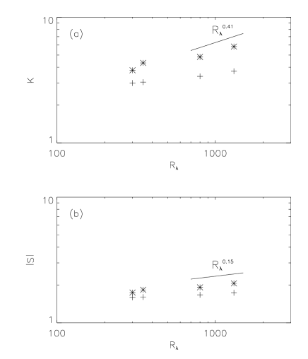
Figure 6: (a) Kurtosis and (b) skewness of the velocity increments as a function of the Taylor based Reynolds number. Results are given for two different increments: the Taylor scale ($+$), and the dissipation scale ($*$). The slopes indicated as a reference are from experimental results.

Figure 4(a) gives the scaling of the flux ratio $\Pi_{\textrm{L}S}(k)/\Pi(k)$ with the Reynolds number. To this end, we take the Taylor scale $\lambda$ as a reference scale in the inertial range, and we evaluate $\Pi_{\textrm{L}S}(k)/\Pi(k)$ for each run at the Taylor wavenumber $k_{\lambda}=2\pi/\lambda$. The best fit to all the runs gives $\Pi_{\textrm{L}S}/\Pi\sim R_{e}^{-0.7}$, although the dependence of the ratio $\Pi_{\textrm{L}S}/\Pi$ with $R_{e}$ seems to change slightly for Run IV. A best fit of the last two points (runs III and IV) gives a dependence $\sim R_{e}^{-0.6}$ (as was discussed in Sect. II, these two runs show a developed inertial range).

We also evaluate the ratio $\Pi_{\textrm{N}L}/\Pi$ at the Taylor wavenumber; its dependence with the Reynolds number is shown in Fig. 4(b). Here, the ratio in runs III and IV is compatible with a slower decay $\sim R_{e}^{-0.4}$. The anomalous behavior of runs I and II in Fig. 4(b) is due to the fact that in these runs at lower resolution, the sum over $P$ from the smallest wavenumber $k_{min}=1$ to $k_{\lambda}/2$ in Eq. (8) defines bands that are too narrow in Fourier space. In other words, it is linked to the lack of a well-defined inertial range in the simulations at lower Reynolds numbers, and we can only expect scaling to obtain in the limit of large $R_{e}$.

Figure 4 indicates that as the Reynolds number is increased, the contribution of the non-local interactions with the large scale flow to the total flux decreases (as well as the contribution of all non-local interactions, albeit at a slower rate). On dimensional grounds $\Pi_{\textrm{L}S}(k_{\lambda})\sim U_{L}u_{\lambda}^{2}/L$. Here, $U_{L}$ is a characteristic velocity at the large scale $L$, and $u_{\lambda}$ is a characteristic velocity at the Taylor scale (note that this relation does not take into account that structures are in fact multiscale Alexakis et al. (2005a)). On the other hand, for $\Pi_{\textrm{L}S}/\Pi\ll 1$, we have $\Pi(k_{\lambda})\sim u_{\lambda}^{3}/\lambda$. As a result, we may expect $\Pi_{\textrm{L}S}(k_{\lambda})/\Pi(k_{\lambda})\sim R_{e}^{-1/2}$. The condition $\Pi_{\textrm{L}S}/\Pi\ll 1$ is not satisfied in the simulations at lower resolution, and it is unclear whether the departure of Run IV in Fig. 4 represents a convergence to a different scaling than $\sim R_{e}^{-0.7}$ at very large Reynolds numbers. This will require further studies at higher numerical resolutions, a feat reachable with petascale computing.

Other scaling laws can be observed in this series of runs; in particular, it is worth comparing the scaling of quantities for which data exist from laboratory experiments or from previous simulations. Figure 5 shows the Kolmogorov constant $C_{K}$ as defined by the inertial range spectrum $E(k)=C_{K}\epsilon^{2/3}k^{-5/3}$. As a reference, we computed a best fit of the form $C_{K}=aR_{e}^{b}+c$, as suggested e.g. in Tsuji (2004), and obtained $a=4.60$, $b=-0.16$, and $c=0.64$. The value of $c$ (that represents the asymptotic value of the Kolmogorov constant for infinite $R_{e}$) obtained from this fit is in good agreement with experimental results and atmospheric observations Mydlarski and Warhaft (1996); Tsuji (2004), although the values of $a$ and $b$ differ. We also note that the measured value of the Kolmogorov constant for the $2048^{3}$ runs is more than double the value of the expected asymptotic limit $c$, indicating that we are still far away from an asymptotic behavior for large $R_{e}$.

Figure 6 shows the skewness

$$S=\left<\delta u_{L}(r)^{3}\right>/\left<\delta u_{L}(r)^{2}\right>^{3/2},$$ (9)

and kurtosis

$$K=\left<\delta u_{L}(r)^{4}\right>/\left<\delta u_{L}(r)^{2}\right>^{2},$$ (10)

of the longitudinal velocity increment $u_{L}={\bf u}\cdot{\bf r}/r$

$$\delta u_{L}(r)=u_{L}({\bf x+r})-u_{L}({\bf x}),$$ (11)

i.e. the component of the velocity in the direction of the increment. The skewness and kurtosis were evaluated at two scales, $r=\lambda$, the Taylor scale, and $r=\eta$, the dissipation scale. In the latter case, only the results from runs III and IV show a dependence with $R_{\lambda}$ which is consistent with experimental results Atta and Antonia (1980). The behavior of these two runs further confirms that high Reynolds numbers are needed to observe scaling of turbulent quantities.

IV Intermittency and structures

The Taylor-Green flows computed here correspond to an experimental configuration of two counter-rotating cylinders, studied in the laboratory for fluid turbulence as well as in the context of the generation of magnetic fields in liquid metals. These flows present both inhomogeneities and anisotropies in the large scales, a resolved inertial range followed by a bottleneck, and a dissipative range. One may study the rate at which the symmetries of the Navier-Stokes equations are recovered in the small scales, and whether the statistical properties of the small scales are universal. In this section we address the specific question of the properties of the small scales through the evaluation of the anomalous exponents $\zeta_{p}$ of the longitudinal structure functions $S_{p}$ of the velocity field, defined as:

$$S_{p}=\langle\delta u_{L}(r)^{p}\rangle\sim r^{\zeta_{p}},$$ (12)

assuming homogeneity and isotropy. In order to obtain better scaling laws, we use the Extended Self-Similarity hypothesis (ESS) Benzi et al. (1993a, b) in the particular context of plotting $S_{p}$ as a function of $S_{3}$.

Figure 7: Scaling exponents using the ESS hypothesis in the $1024^{3}$ and $2048^{3}$ runs. The scaling predicted by Kolmogorov and by the She-Lévêque model are also given as a reference.

Figure 7 shows the scaling exponents $\zeta_{p}$ in the $1024^{3}$ and $2048^{3}$ runs, computed using the ESS hypothesis. Similar results are obtained without ESS and doing the fit only in the inertial range, defined as the range of scales where the so-called 4/5th law of Kolmogorov is satisfied, namely $S_{3}(r)\sim r$. If we define stronger intermittency as stronger departure from the Kolmogorov scaling $\zeta_{p}=p/3$, we note that as we increase the Reynolds number, the intermittency increases as well, albeit slowly. Furthermore, for higher $R_{\lambda}$ (run IV), the departure from the She-Lévêque model She and Lévêque (1994) increases (compared with run III), even for fixed values of $p$. The differences between $\zeta_{p}$ for runs III and IV, albeit small, are at least one order of magnitude larger than the errors in the fit using ESS. As an example, in run III $\zeta_{6}=1.746\pm 0.003$ and $\zeta_{8}=2.136\pm 0.007$, while in run IV $\zeta_{6}=1.7284\pm 0.0004$ and $\zeta_{8}=2.0968\pm 0.0007$.

Here it is worth separating the discussion in two parts. On the one hand, the increase of the departure from the She-Lévêque model as the Reynolds number and spatial resolution are increased indicates that the departure is not the result of lack of statistics. This change in the exponents for simulations with the same forcing at different Reynolds numbers shows that huge Reynolds are required to obtain convergence of high order statistics. In fact, the larger the moment $p$ examined, the larger the relative difference between the $\zeta_{p}$ exponents measured in the two runs. On the other hand, it was shown in Ref. Mininni et al. (2006) that differences in the scaling exponents were measurable when considering two different forcings at similar Reynolds numbers. These differences could be due to anisotropies in the flow, and in that case an SO(3) decomposition could be used to study whether the scaling exponents of the isotropic component of the flow are universal. However, if there is a significant return to isotropy in the small scales, we then also expect the isotropic component to dominate when the Reynolds number is large enough.

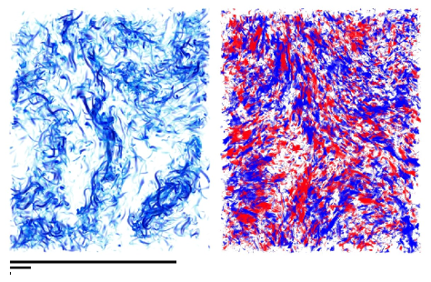
Figure 8: (Color online) Left: rendering of vorticity intensity in a small region of run IV. Only regions with $|\bm{\omega}|\geq\max\{|\bm{\omega}|\}/6.5$ are shown ($\bm{\omega}=\nabla\times{\bf v}$). Note the clustering of filaments into larger vorticity structures. The bars on the bottom indicate respectively the integral, Taylor, and dissipation scales. Right: rendering of relative helicity in the same region (red is $-1$ and blue is 1). Only regions with absolute value larger than $0.92$ are shown.

The intermittency of the flow is linked to the presence of strong spatially separated structures in the form of vortex filaments. The high $R_{\lambda}$ computation (run IV) displays the same large-scale structure of bands as the run presented in Mininni et al. (2006). Conditional statistics analysis as the ones performed in Mininni et al. (2006) keep showing a correlation between large scale shear and small scale gradients and enhanced intermittency. It has been noted by several authors that filaments tend to cluster into larger filamentary structures; this is observed e.g. for supersonic turbulence Porter et al. (1998) and in the interstellar medium, and it has been analyzed quantitatively in Moisy and Jiménez (2004). When individual structures are studied in real space, filament-like clusters formed by smaller vortex filaments are observed here again (see Fig. 8), something that was not seen in simulations of the TG flow at lower resolution. This could be interpreted as a manifestation of self-similarity, and a more quantitative analysis will be presented elsewhere. In particular, it would be of interest to compute the inter-cluster distance, and the intra-cluster inter-filament distance, to see whether the space-filling factor of such flows diminish with increasing Reynolds number. Note that the vortex cluster reaches a global length comparable to the integral scale of the flow (indicated in Fig. 8); as such, they may be a real-space manifestation of the trace of non-local interactions between small-scales (dominated by vortices) and large scales (dominated by the forcing), giving a coherence length to the flow.

Figure 8 also shows the density of relative helicity ${\bf v}\cdot\bm{\omega}(|{\bf v}||\bm{\omega}|)^{-1}$ ($\bm{\omega}=\nabla\times{\bf v}$). Regions in blue and red correspond respectively to regions of maximum alignment or anti-alignment between the two fields (only regions with absolute relative helicity larger than $0.92$ are shown). Note that regions with large relative helicity correspond to small vortex tubes, but the filament-like clusters have no coherent helicity. Regions with strong alignment fill a substantial portion of the subvolume, even though the global (relative) helicity of the flow is close to zero.

V Discussion and Conclusion

The data presented in this paper has allowed for a refined analysis of the behavior and structure of turbulent flows as the Reynolds number is increased. We have in particular showed that: (i) the bottleneck appears to have a constant width for the two higher $R_{e}$ runs; hence, it is probably linked to the dissipation range, and to the depletion of nonlinearities as we approach this range; (ii) the scaling with $R_{e}$ of the non-local energy fluxes, which indicates a weakening of non-local interactions as $R_{e}$ increases. These first two results taken together point out to the fact that the bottleneck may not disappear in the limit of very high Reynolds number, since it has been argued that its existence is linked to the relative scarcity of non-local interactions in Navier-Stokes turbulence, by opposition to, e.g., the magnetohydrodynamic (MHD) case. Indeed, when coupling the velocity to a magnetic field in the MHD limit, it was shown that the transfer of energy itself was non-local, and that the bottleneck was absent in numerical simulations of such flows; this can be understood in the following manner: as one approaches the dissipation range, few triadic interactions are available but in a flow for which the nonlinear transfer is nonlocal, the energy near the dissipative range can still be transfered efficiently to smaller scales since small-scale fluctuations are transfered by the large scales Alexakis et al. (2005b). Finally, the departure of the anomalous exponents of velocity structure functions from standard models of intermittency such as the She-Lévêque model seems to increase as the Reynolds number is increased.

As noted before in Kaneda and Ishihara (2006), convergence to the asymptotic turbulence regime appears to be very slow: even though the nonlocal interactions do diminish with Reynolds number, they are still measurable at these resolutions. In run IV on a $2048^{3}$ grid at $R_{\lambda}\sim 1300$, of the order of $10\%$ of the energy flux is due to non-local interactions with the large scale flow, and the dependence of the energy flux ratio $\Pi_{\textrm{L}S}/\Pi$ with $R_{e}$ for very large $R_{e}$ is still unclear. This not only raises the question of the determination of higher order quantities at moderate Reynolds numbers in simulations and experiments, but it also opens the door for a non-universal behavior of turbulent flows which may have to be studied in more detail than was previously hoped for.