The central parsecs of Centaurus A:
high excitation gas, a molecular disk, and the mass of the black hole

Abstract

We present two-dimensional gas-kinematic maps of the central region in Centaurus A. The adaptive optics (AO) assisted SINFONI data from the VLT have a resolution of $0\farcs 12$ in K-band. The ionized gas species (Br$\gamma$, [Fe ii], [Si vi]) show a rotational pattern that is increasingly overlaid by non-rotational motion for higher excitation lines in direction of Cen A’s radio jet. The emission lines of molecular hydrogen (H₂) show regular rotation and no distortion due to the jet. The molecular gas seems to be well settled in the gravitational potential of the stars and the central supermassive black hole and we thus use it as a tracer to model the mass in the central $\pm 1\farcs 5$. These are the first AO integral-field observations on the nucleus of Cen A, enabling us to study the regularity of the rotation around the black hole, well inside the radius of influence, and to determine the inclination angle of the gas disk in a robust way. The gas kinematics are best modeled through a tilted-ring model that describes the warped gas disk; its mean inclination angle is $\sim 34\arcdeg$ and the mean position angle of the major axis is $\sim 155\arcdeg$. The best-fit black hole mass is $\rm{M_{BH}=(4.5^{+1.7}_{-1.0})\times 10^{7}M_{\odot}}$ (3$\sigma$ error), based on a “kinematically hot” disk model where the velocity dispersion is included through the Jeans equation. This black hole mass estimate is somewhat lower than, but consistent with the mass values previously derived from ionized gas kinematics. It is also consistent with the stellar dynamical measurement from the same AO observations, which we present in a separate paper. It brings Cen A in agreement with the $\rm{M_{BH}-\sigma}$ relation.

1. Introduction

During the last few years it has been realised that most, if not all, nearby luminous galaxies host a supermassive black hole (BH) in their nuclei with masses in the $10^{6}-10^{10}M_{\odot}$ range (e.g. Ferrarese & Ford, 2005, and references therein). The black hole mass ($\rm{M_{BH}}$) is tightly related with mass or luminosity of the host stellar spheroid, bulge, (e.g. Kormendy & Richstone 1995; Marconi & Hunt 2003; Häring & Rix 2004) and with the stellar velocity dispersion, $\sigma$, (Ferrarese & Merritt, 2000; Gebhardt et al., 2000). These correlations have an amazingly low scatter, perhaps surprisingly low, since the quantities $\rm{M_{BH}}$ and $\rm{M_{bulge}}$/$\sigma$ probe very different scales. These facts indicate that the formation of a massive BH is an essential ingredient in the process of galaxy formation.

The mass of the black hole at the center of NGC 5128 (Centaurus A), the most nearby elliptical galaxy, is still under debate. Centaurus A hosts a powerful radio source and an AGN revealed by the presence of a powerful radio and X-ray jet (see Israel 1998, for a review; see also Tingay et al. 1998; Hardcastle et al. 2003; Grandi et al. 2003; Evans et al. 2004, and references therein). Recent stellar dynamical measurements and modeling by Silge et al. (2005) result in a black hole mass of 2.4$\times 10^{8}M_{\odot}$ (for an edge-on model), while different gas-dynamical studies found masses in the range of $6.1\times 10^{7}M_{\odot}$ to $2\times 10^{8}M_{\odot}$ depending mainly on the inclination angle of the modeled gas disk (Marconi et al., 2001, 2006; Häring-Neumayer et al., 2006; Krajnović et al., 2007). Given a velocity dispersion for NGC 5128 of 138 km s^-1 (Silge et al., 2005), we would expect a BH mass around $3\times 10^{7}M_{\odot}$ from the $\rm{M_{BH}-\sigma}$ relation. If this BH mass is correct, NGC 5128 has the largest offset from the $\rm{M_{BH}-\sigma}$ relation ever measured (taken the mass values of Marconi et al. (2001) and Silge et al. (2005)). Based on its stellar velocity dispersion and the black hole mass expected by the $\rm{M_{BH}-\sigma}$ relation the radius of influence of Cen A’s black hole is $\sim 0\farcs 3$. Thus, ground based, seeing limited observations are not suitable to resolve this radius. Using high-spatial resolution ($\sim 0\farcs 1$) ionized gas kinematics from adaptive optics assisted and space based observations, Häring-Neumayer et al. (2006) and Marconi et al. (2006) find masses reduced by a factor 3-4 compared to previous measurements. They were, however, limited to long-slit data at a few position angles and not able to precisely constrain the inclination angle of the modeled gas disk. With the availability of integral-field spectroscopy (IFS) in the near infrared (IR) the gas as well as the stars can be mapped in two dimensions even in dust-shrouded galaxy centers, like Cen A. Black hole masses can be derived separately from stars and gas from the same complete data set, and the gas geometry is constrained by two-dimensional data. The star and gas results can then be compared to assess the reliability of the modeling techniques. SINFONI (Eisenhauer et al., 2003a, b; Bonnet et al., 2004) at the Very Large Telescope (VLT) combines IFS with the resolving power of adaptive optics assisted observations and provides data at a spatial resolution of $\sim 0\farcs 1$ in K-band. For Cen A the radius of influence of the black hole at the center should be comfortably resolved. Still, this resolution is far from anywhere near the Schwarzschild radius of the black hole and cannot constrain the central object to be a black hole. However, Cen A ranks among the best cases for a supermassive black hole in galactic nuclei (see Marconi et al. 2006 for a discussion.)

For our dynamical model we assume a distance to NGC 5128 of 3.5 Mpc to be consistent with all previous mass determinations. Recent distance measurements are in the range 3.4 Mpc to 4.2 Mpc (Israel, 1998; Tonry et al., 2001; Rejkuba, 2004; Ferrarese et al., 2007), with typical uncertainties of $\sim 8\%$. At the assumed distance of 3.5 Mpc, 1 arcsecond corresponds to $\sim$17pc.

This paper is a follow-on to the work presented in Häring-Neumayer et al. (2006) (hereafter HN+06), using high spatial resolution Naos-Conica (NaCo) imaging and spectroscopy data to get an accurate measurement of Cen A’s black hole mass. While the analysis of HN+06 was restricted to [Fe ii]  kinematics along 4 long slit positions, we study in detail the kinematics of different gas species at the center of NGC 5128 in two dimensions. Unsurprisingly, different gas species exhibit different behaviors. While the (highly) ionized gas shows (strong) influence by the jet (both in surface brightness and in the kinematic maps), the molecular gas (H₂) seems to “feel” only gravity. This is the reason why we focus on H₂ when we construct a dynamical model to measure the mass of the central supermassive black hole. Moreover, the two-dimensional data allow us to determine the inclination angle of the gas disk in a robust way. Taken together, these advancements over the work of HN+06 and other previous studies, greatly decrease the overall uncertainty in Cen A’s black hole mass measurement. SINFONI stellar kinematics and black hole mass modeling are consistent with the gas-dynamical study and black hole mass measurement presented here, and will be presented in a separate paper (Cappellari et al., in prep.).

The paper is organized as follows: Section 2 describes the observations and the data reduction. Section 3 presents the gas morphology and kinematics and Section 4 our dynamical model. Section 5 gives the modeling results and Section 6 discusses them.

2. Observations and Data Reduction

All observations presented here were taken with SINFONI on the UT4 (Yepun) of the VLT of the European Southern Observatory (ESO) at Cerro Paranal, Chile, on March 23 and April 1, 2005. SINFONI consists of a cryogenic near-infrared integral field spectrometer SPIFFI (Eisenhauer et al., 2003a, b) coupled to the visible curvature adaptive optics (AO) system MACAO (Bonnet et al., 2003). For the Cen A nucleus, the SINFONI AO module was able to correct on an R$\sim$14mag star $36\arcsec$ South-West of the nucleus in excellent seeing of $0\farcs 5$, reaching nearly the diffraction limit of the telescope in the K band. With the appropriate pixel scale selected ($0\farcs 05\times 0\farcs 1$ per spatial element), the spectrograph was able to obtain spectra across the entire K band (approximately $\lambda$1.93-2.47$\mu$m) at a spectral resolution of R$\sim$4000 and covering a $3\arcsec\times 3\arcsec$ field of view, in a single shot. A total of 10 sky (S) and 15 on-source (O) exposures of 900 s each followed a sequence OSO… and were dithered by only a few pixels to allow removal of bad pixels and cosmic rays. The frames were combined to make the final K band data cube with a total on-source exposure of 13500 s.

In the same way, we obtained H-band data ($\lambda$1.43-1.87$\mu$m) with a slightly lower spectral resolution of R$\sim$3000 covering the central $3\arcsec\times 3\arcsec$ with a scale of $0\farcs 05\times 0\farcs 1$ per pixel. The overall integration time for H-band was 3600 s.

The data were reduced using the SINFONI data reduction pipeline provided by ESO. The nearest sky exposure was subtracted from the object frames, after which the data was flatfielded and corrected for bad pixels. Distortion correction was done based on the position of OH line edges in sky frames. The wavelength calibration was based on the nightsky OH lines in H-band and on OH lines and arc lamp frames in K-band. Using the slitlet positions derived from the sky frames and the obtained wavelength calibration a three-dimensional data cube were created from each object frame. Finally the slitlet positions were adjusted if necessary based on crosscorrelation with NaCo broadband images (taken from HN+06). The typical shift between the slitlets is in the range of $\sim 0.1-0.3$ pixels. This correction is applied to retain the full spatial resolution of the data. After correcting for telluric features and flux calibration the data cubes were mosaicked together. The stars Hip079775 (B3III) and Hip68359 (B8V) were used both as telluric standards and flux calibrators. The flux calibration has an accuracy of about 5-10%.

2.1. Spatial resolution

To assess the spatial resolution of the data, the point-spread function (PSF) is estimated from the unresolved active galactic nucleus (AGN), as discussed in more detail by HN+06. No additional PSF calibration frames using stars were taken, since the PSF in adaptive optics observations depends on several factors such as atmospheric conditions, brightness of and distance to the guide star, contrast of the guide star to the background, and these conditions are difficult to duplicate for the science and calibration observations. The most accurate measure of the science frame PSF in the vicinity of the AGN is therefore achieved directly on the unresolved nucleus.

We describe the normalized PSF empirically by a sum of two Gaussian components; one narrow component describing the corrected PSF core ($\sigma_{\rm{c}}$) and one broader component ($\sigma_{\rm{s}}$) which can be attributed to the seeing halo plus extended emission:

$$PSF(r)=\rm{\frac{F}{2\pi\sigma^{2}_{c}}e^{-r^{2}/2\sigma^{2}_{c}}+\frac{(1-F)}{2\pi\sigma^{2}_{s}}e^{-r^{2}/2\sigma^{2}_{s}},}$$ (1)

where F is the ratio of the flux of the narrow component and the total flux of the PSF (F = $\rm{flux_{c}/flux_{total}}$). The quantity F provides a rough approximation of the Strehl ratio (S) which gives the quality of an optical system; S is defined as the observed peak flux divided by the theoretically expected peak flux of the Airy disk for the optical system (S = $\rm{peakflux_{c}/peakflux_{Airy}}$). For the following analysis it is sufficient to measure the quantity F, which also gives an estimate of the quality of the adaptive optics correction.

For the K-band cube, a PSF model of the above form is fitted to the peak in surface brightness in the collapsed wavelength range of $\lambda$2.00 to 2.10 $\mu m$ (just next to the H₂ line). The two components of the PSF model shown in comparison to the data in Fig. 1 have a full width at half maximum (FWHM) of $0\farcs 12$ and $0\farcs 30$, for the narrow and broad component respectively. The estimated Strehl ratio is 17%. The width of the broad component compares well to the FWHM of the seeing disk as measured by the seeing monitor during the observations (FWHM${}_{V}\sim 0\farcs 5$ transformed to K-band as in HN+06, FWHM${}_{K}\sim 0\farcs 38$).

Figure 1.— Double Gaussian fit of the K-band SINFONI PSF on the continuum just next to the H₂ line. The FWHM of the narrow and broad component is $0\farcs 12$ and $0\farcs 30$, respectively. The estimated Strehl ratio is 17% (see Section 2.1 for a definition of these quantities)

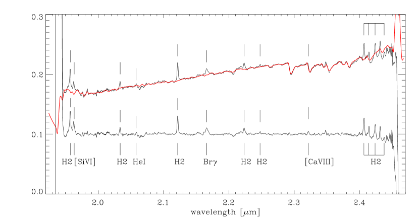
2.2. Subtraction of the stellar and non-stellar continua

The total or averaged spectrum of the central $0\farcs 8\times 0\farcs 8$ of Cen A (Fig. 2) shows strong CO absorption lines at 2.3-2.4 $\mu m$ indicating the stellar continuum. We use the penalized pixel fitting method (pPXF) of Cappellari & Emsellem (2004) to fit the stellar continuum with a positive linear combination of stellar templates. As template stars serve six late type stars that were observed with SINFONI in the same setup that we used for the nucleus of Cen A. This ensures that the instrumental spectral broadening is the same for the template stars and the galaxy spectrum, and we need not know the underlying instrumental line profile.

As possible template stars we chose the following: K3V, M0III, M0V, M4V, M5II, and M5III. The wavelength regions with emission lines were omitted from the fit and the optimal template was convolved with Gauss-Hermite expansions (van der Marel & Franx, 1993; Gerhard, 1993) up to h₄, minimizing the difference between the galaxy spectrum and the template.

In addition to the stellar continuum, the non-stellar continuum is fitted via an additive Legendre polynomial of fourth order. This becomes important in the central region where the power-law continuum of the AGN dominates the flux distribution.

Figure 2.— K-band spectrum of the nucleus of Cen A integrated over a square aperture of $0\farcs 8\times 0\farcs 8$. The best-fitting composite spectral template (a mix of stellar spectra and a featureless continuum) is overplotted in red. The residual, reflecting the pure emission line spectrum, is shown in the lower part, with the main emission lines identified. Note the strong CO absorption that is very well fitted by the stellar template

After the subtraction of the stellar and non-stellar continuum we are left with a data cube of pure emission line spectra.

2.3. Extraction of the gas emission lines

The SINFONI Cen A spectra in the wavelength range $\lambda$1.43-1.87$\mu$m and $\lambda$1.93-2.47$\mu$m (the H- and K-band, respectively) exhibit a wealth of gas emission lines. High excitation lines such as [Si vi]  and [Ca viii], ionized gas emission lines ([Fe ii], Br$\gamma$, He i), and several transitions of molecular hydrogen H₂  are detected (Figure 2). In this paper we focus on the kinematic properties of [Si vi], Br$\gamma$, [Fe ii], and H₂  and show that they have quite different kinematics. While the high-excitation lines appear to be affected, or created, by Cen A’s jet, the H₂ gas appears to be solely rotating. We construct a dynamical model to explain the kinematics of the strongest line of molecular hydrogen 1-0 S(1) H₂ at $\rm{\lambda=2.122\mu m}$ and use this to measure the mass of the supermassive black hole at the center of NGC 5128. Single Gaussians provide a good fit to the emission lines and are used to measure the central wavelength, width and intensity of each line independently. The fit is performed in IDL using a non-linear least squares fit to the line and the errors are the 1-$\sigma$ error estimates of the fit parameters. The typical uncertainties of the peak flux and the width of the lines are  3-5%, whereas the position of the line ca be determined to less than 1% accuracy. This translates to a typical uncertainty in the velocity of the molecular hydrogen line of $\sim\pm$5 km s^-1 and in the velocity dispersion of $\sim\pm$10 km s^-1.

To allow for the best possible extraction of the gas lines the extraction window is centered on the expected wavelength. Its width is optimized iteratively to fully cover the width of the line and to make sure the extraction window covers the same range on the left and right of the line peak. An initial estimate of the Gaussian fit parameters (amplitude, central position, and width) was derived from a smoothed spectrum at a central position in the velocity field, near the AGN, and applied as a starting value throughout the field. This initial estimate is introduced in order to prevent fitting of spurious lines in the regions of bad pixels or strong continuum variation.

The signal-to-noise ratio of the spectra appears high enough for extracting the gas emission lines and drops rapidly to zero. Therefore, we do not spatially bin the data. We only consider the detection of the lines to be secure when their amplitude is a factor of 3 above the RMS scatter of the spectrum (A/N$\geq$3). In this way we get an accurate fit to the lines over the entire field, with typical uncertainties of a few percent.

3. Emission-line gas measurements

From the parameters of the Gaussian fit - peak value, mean wavelength and width - we get the flux (or, surface brightness), the velocity and the velocity dispersion for the considered gas species, [Si vi], Br$\gamma$, [Fe ii], and H₂. Since the stellar and non-stellar continua have been subtracted, the line-flux is directly measured as $\sqrt{2\pi}\rm{F_{peak}}\sigma$. For the velocity, we take the recession velocity of Cen A’s stellar body (v${}_{\rm{sys}}=532\pm 5$ km s^-1, Marconi et al. 2001) as the reference and measure all line shifts with respect to this velocity.

3.1. Gas kinematics

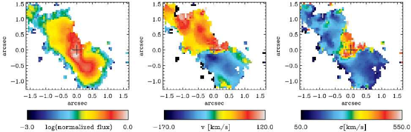
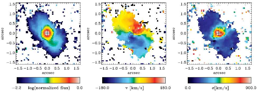
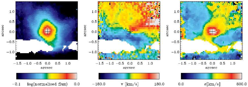
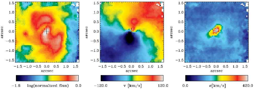
Figures 3-6 show the maps of total flux, velocity, and velocity dispersion for the detected lines of [Si vi], Br$\gamma$, [Fe ii], and H₂. These line maps illustrate vividly how the flux distribution and kinematics change when going from high- to low-excitation states. The highest excitation line, [Si vi], is dominated by a non-rotational component.

When comparing the velocity fields of [Si vi], [Fe ii], and H₂, (middle panel in Figures 3-6) one notices that the velocity field of [Si vi]  consists of two major components: rotational and translational motion. The velocity fields of [Fe ii]  and Br$\gamma$  are dominated by rotation but are still distorted by a non-rotational component that is strongest to the lower right (south-west) of the field (blue component). These non-rotational motions seen in [Si vi], [Fe ii], and Br$\gamma$  are located close to the projected direction of the radio jet in Centaurus A (P.A.=51$\arcdeg$ Clarke et al. 1992; Tingay et al. 1998; Hardcastle et al. 2003). The measured values for the inclination angle of the jet vary between $50\arcdeg<i<80\arcdeg$ (Tingay et al., 1998, from VLBI data) and $20\arcdeg<i<50\arcdeg$ (Hardcastle et al., 2003, from VLA data), but without doubt the North-Eastern part is pointed towards us. Surprisingly, the direction of motion seen in [Si vi]  is red-shifted in the jet pointing towards us and blue-shifted in the counter-jet. Under the plausible assumption that the geometries of the jet and [Si vi], are aligned, this indicates an inflow of material towards the nucleus.

This inflow motion could be associated with backflow of gas that was accelerated by Cen A’s jet and after producing a bowshock is flowing back at the side of the jet cocoon. Although on much larger scales, this phenomenon is seen in jet simulations (e.g. Krause, 2005). As the gas is flowing back, it is reionized by radiation from the central source. This was proposed by Taylor et al. (1992) as a mechanism to produce the narrow line regions in Seyfert galaxies.

While the kinematics of the very high and medium ionization lines [Si vi]  and [Fe ii]  are manifestly influenced by this jet induced motion, the velocity field of H₂  shows no distortion due to the jet. The velocity field is very smooth and symmetric and indicative of rotation, with a striking twist of the major kinematic axis around a median P.A.=$155\arcdeg$. However, the velocity fields in all the other gas tracers give evidence that at least part of that gas rotates in a nuclear gas disk. Moreover, the velocity dispersion maps of [Si vi], Br$\gamma$, [Fe ii], and H₂  support the picture of an inclined nuclear gas disk. They all show an elongated structure in their high dispersion component, mimicking a disk, at a position angle of $125\pm 25\arcdeg$, and a declining dispersion profile outwards. The ionized gas species ([Si vi], [Fe ii], and Br$\gamma$) show in addition a colder component (with $\sigma\sim 150$ km s^-1) that is elongated in the direction of the translational motion. Although being as high as $\sigma\sim 400$ km s^-1, the velocity dispersion of H₂ has the lowest central value. It is not clear what causes this high velocity dispersion for the molecular gas (see also 4.2). Nevertheless, H₂ shows the most ordered structure both in the maps of velocity dispersion and mean velocity and it seems to be well settled in a disk.

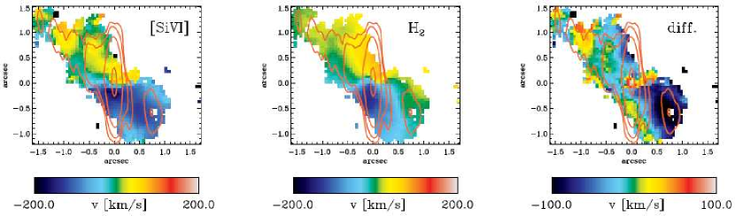
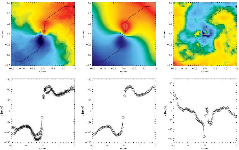
To visualize the difference in the velocity pattern of [Si vi]  and H₂  Figure 7 shows the comparison of the H₂  and [Si vi]  velocity fields (left and middle panel) masked with the [Si vi]  flux map. The right panel shows the direct difference $v(\mbox{[Si\,{\sc vi}]})-v(\mbox{H${}_{2}$})$. Overplotted are the VLA contours of the radio jet (unpublished VLA data kindly provided by M. Hardcastle). The non-rotational component of the [Si vi]  velocity field becomes strongest SW of the nucleus, and can be identified with the innermost knot in the VLA radio jet. We most likely see evidence for jet-gas cloud interaction in the ionized gas species.

3.2. Gas morphology

Looking at the flux maps of the gas species, one notices the very different morphologies in the high- and low-ionization lines. The morphology of [Si vi]  is dominated by an elongated structure that extends south-west of the nucleus, at a position angle of $\sim 33\arcdeg$. This structure widens and ends in a blob or knot at $\sim 1\arcsec\simeq 17$pc from the center. The position of this knot is coincident with the innermost knot in the radio counterjet south-west of the nucleus (seen by Clarke et al. (1992) and denoted SJ1 by Hardcastle et al. (2003)).

Overall, the morphology of Br$\gamma$  and [Fe ii]  (Figures 4 and 5) resemble that of [Si vi]  very closely, but overall the elongation is not as pronounced and the structure appears rounder.

For all gas species, the P.A. of the elongation is $\sim 33\arcdeg$ which is the same as for the elongated structure detected in Pa$\alpha$ by Schreier et al. (1998), that is centered on the nucleus and extended by $\pm 2\arcsec$. They interpret this as an inclined, $\sim$40 pc diameter, thin nuclear disk of ionized gas rather than a jet-gas cloud interaction. However, our 2D data show that the gas moves along this elongated structure that extends around the jet axis. The direction of motion hints towards a backflow of jet material onto the accretion disk as mentioned above.

In addition to this elongated structure, our high spatial resolution integral field data show evidence for a nuclear disk of ionized and molecular gas oriented approximately perpendicular to the jet angular momentum vector. Looking at the central $0\farcs 5\times 0\farcs 5$ of the H₂  flux map (Fig. 6), one notices a disk-like structure with a major axis of $\sim 140\arcdeg$. The same structure is visible in the Br$\gamma$  and [Fe ii]  flux maps, although a bit rounder. Looking at the whole H₂  flux distribution, it appears very different from the ionized gas species, and the shells at the upper left and lower right are a dominant feature. These shells are reminiscent of the bowshock structures seen at larger scales in the outer regions of radio jets (e.g. Carilli et al., 1988, for Cyg A) and on smaller scales in Herbig-Haro objects (e.g. Reipurth et al., 2002). They are located at a (projected) position where the elongated structure in [Si vi], Br$\gamma$, and [Fe ii]  disappears. This is another hint towards the bowshock model of Taylor et al. (1992) where the shocked gas (here [Si vi], [Fe ii], and Br$\gamma$) flows back towards the nuclear source along the shell. It is important to note that although the shells dominate the appearance of the H₂  flux map, they do not leave any kinematic signature in the H₂  velocity field.

Figure 3.— Surface brightness, velocity, and velocity dispersion maps of the [Si vi]  line emission (left, middle, right panel, respectively). The surface brightness map is displayed in logarithmic scaling. The velocities and velocity dispersions are only plotted for the regions that are above the lower flux limit displayed in the left panel. The velocity scale is given relative to the systemic velocity of the galaxy (532 km s^-1). The velocity dispersion is corrected for the instrumental dispersion ($\sigma_{\rm{instr}}\approx 65$ km s^-1). North is up and East is to the left

Figure 4.— Flux, velocity, and velocity dispersion maps of Br$\gamma$. See caption of Fig. 3 for more details

Figure 5.— Flux, velocity, and velocity dispersion maps of [Fe ii]. See caption of Fig. 3 for more details. We masked out an artifact around y$\sim-0\farcs 7$ that is caused by illumination effects on the SINFONI detector

Figure 6.— Flux, velocity, and velocity dispersion maps of H₂. See caption of Fig. 3 for more details

Figure 7.— Comparison between the [Si vi]  (left) and H₂  (middle) velocity fields with their difference shown in the right panel. The velocity fields are masked with the [Si vi]  flux map which nearly coincides with the radio jet (red contour overlay [unpublished VLA data kindly provided by M. Hardcastle]). The differenced velocity field (right hand panel), meant to ‘correct’ the [Si vi]  kinematics for their rotational component, reveals a distinct [Si vi]  velocity gradient along the jet. The blue component SW of the AGN ($0\farcs 7$,$-0\farcs 6$) marks the strongest translational velocity component, matching the knot in the radio jet

4. Gas Dynamical Modeling

While the (highly) ionized gas shows (strong) kinematic influence by the jet, the molecular gas (H₂) seems to “feel” only gravity. This is the reason why we focus on H₂ when we construct a dynamical model to measure the mass of the central supermassive black hole.

4.1. Method

The dynamical model follows the approach of HN+06 and uses two-dimensional SINFONI gas kinematic maps as constraints. In brief: to explain the H₂  gas motions seen in the center of Cen A we construct a kinematic model where we assume the gas moves in a thin disk solely under the gravitational influence of the surrounding stars and the expected central black hole. Then, the gravitational potential is given as $\Phi(r)=\Phi_{\star}(r)+\Phi_{\rm{BH}}(r)$. The stellar potential $\Phi_{\star}$ is taken from HN+06, where NaCo, NICMOS, and 2MASS K-band images of NGC 5128 are used to construct a Multi-Gaussian Expansion (MGE) parameterization to the surface brightness of this galaxy (Emsellem, Monnet, & Bacon, 1994; Cappellari, 2002a). The assumptions of spherical symmetry and constant stellar mass-to-light ratio ($\rm{M/L_{K}=(0.72\pm 0.04)}$ $\rm{M_{\odot}/L_{\odot}}$ (Silge et al., 2005); HN+06) lead to the three-dimensional mass model, that gives the stellar velocity contribution to the dynamical model.

Our dynamical model is based on the widely used approach to model the emission line profile of gas moving in a thin disk (Macchetto et al., 1997; van der Marel & van den Bosch, 1998; Bertola et al., 1998; Barth et al., 2001). In HN+06 we considered three conceptual modeling approaches: 1) a cold disk model that fully neglects the velocity dispersion, 2) a hot disk model that accounts for the high velocity dispersion of the gas, and 3) a spherical Jeans model that accounts for the high velocity dispersion but neglects the indicated disk geometry. We do not repeat the spherical Jeans model here, as the H₂  velocity maps clearly require a disk model. Since the observed velocity dispersion even of the H₂  gas at the nucleus of Cen A exceeds the mean rotation by more than a factor of two, we must account for the velocity dispersion in the dynamical model. We assume the gas disk to be geometrically flat but with an isotropic pressure and construct an axisymmetric Jeans model in hydrostatic equilibrium. In this case, the mean rotation velocity (azimuthal velocity) $\overline{v_{\Phi}}$ is given by the Jeans equation (Binney & Tremaine, 1987, Eq.4-64a)

$$\overline{v_{\Phi}}^{2}=\frac{R}{\rho_{g}}\frac{\partial(\rho_{g}\sigma_{R}^{2})}{\partial R}+R\frac{\partial\Phi}{\partial R},$$ (2)

where $R$ is the projected radius and $\sigma_{R}$ is the radial velocity dispersion of the gas. We assume that the H₂ surface brightness of the gas disk $\Sigma_{g}$ reflects the tracer gas density $\rho_{g}$ (see Section 4.3 for a discussion). Note that the model is not self-consistent, i.e. the contribution of the gas mass to the overall potential is neglected. We estimate the mass inside the SINFONI field-of-view, following Israel et al. (1990). They identify a central H₂  gas disk with an outer radius of $\sim 6\farcs 5$, a thickness of $\sim 3\farcs 3$, and an inner cavity of $\sim 1\farcs 7$ (assuming a distance to Cen A of D=3.5 Mpc), and with a density distribution of $\rho(r)\sim r^{-2}$. The total disk mass is $2\times 10^{7}M_{\odot}$. To get a first order estimate of the mass inside the central $3\arcsec\times 3\arcsec$ we assume a constant density throughout the disk and neglect the inner cavity, which is not confirmed by our data. Inside the field of view of our SINFONI observations we therefore expect $M_{\mbox{H${}_{2}$}}\sim 1\times 10^{6}M_{\odot}$, which is a factor of 60 to 200 smaller than the black hole mass measurements for Cen A (HN+06; Marconi et al. 2001), and therefore negligible.

To match the observations, the resulting velocity field can then be projected onto the plane of the sky, given the inclination angle $i$ and the position angle (P.A.) of the projected major axis of the gas disk. For comparison with the data, the projected velocity field must also be broadened with the velocity dispersion and then weighted by the gas surface brightness, using the parameterizations given subsequently in Sections 4.2 and 4.3, respectively. Finally, we simulate observations of the disk through the SINFONI instrument, i.e. we convolve with the SINFONI PSF and sample over the pixel size, to achieve the best possible match to the data. The model thus has three free parameters, the black hole mass $\rm{M_{BH}}$, the inclination angle of the disk $i$, and its projected P.A. $\zeta$. The galaxy center position on the detector (defined as the continuum peak) and the stellar mass-to-light ratio are fixed beforehand, with $\rm{M/L_{K}=0.72}$ $\rm{M_{\odot}/L_{\odot}}$ as described above. To measure the black hole mass in NGC 5128, we run models with different values for the free parameter and look for the best possible match to the data, minimizing the $\chi^{2}$ .

For the modeling we use the IDL software of HN+06, which accounts for the SINFONI PSF (as determined in Section 2.1), instrumental broadening, and the finite SINFONI pixel size, to generate a two-dimensional model spectrum with the same pixel scale as the observations. The extraction of the mean velocity and velocity dispersion from this synthetic data cube is carried out in exactly the same manner as for the observed data, by fitting single Gaussians to the individual spectra at each pixel.

4.2. Intrinsic gas velocity dispersion

The observed velocity dispersion of the molecular hydrogen H₂  gas at the center of NGC 5128 peaks at 400 km s^-1 and exceeds the measured mean rotational velocity by more than a factor of two (for comparison: the ionized gas species [Fe ii]  used in the study of HN+06, has a peak velocity dispersion of $\sim$ 600 km s^-1). The physical origin of this high velocity dispersion is not clear. Partially it might be explained by spatially unresolved rotation (Marconi et al., 2001, 2006), or it might be due to local turbulent gas motions, as suggested by several authors for other galaxies (e.g. Barth et al., 2001; van der Marel & van den Bosch, 1998; Verdoes Kleijn et al., 2002), which appears problematic especially for the H₂.

Regardless of its physical cause, we consider the high velocity dispersion to contribute to the pressure support of the gas disk. Following the approach of HN+06 we include the velocity dispersion to the gas dynamical model via an isotropic pressure term in the Jeans equation. The rotational velocity therefore becomes sub-Keplerian. We find that the intrinsic velocity dispersion is well described by a double exponential profile of the form

$$\sigma_{R}=\sigma_{0}e^{-r/r_{0}}+\sigma_{1}e^{-r/r_{1}},$$ (3)

and we fit the observed H₂, velocity dispersion profile for the best set of parameters ($\sigma_{0}$=140 km s^-1, $\sigma_{1}=65$ km s^-1, $r_{0}=0\farcs 25$, and $r_{1}=4\farcs 0$) to get the intrinsic dispersion profile.

4.3. Emission line surface brightness

For various aspects of the modeling, we need to know the intrinsic spatial emission line profile (assumed to be axisymmetric). But a direct deconvolution of the observed surface brightness is very difficult, since for adaptive optics observations the exact shape of the PSF is unknown and we would therefore introduce artifacts to the gas distribution that bias the velocity distribution inside the inner $0\farcs 5$.

Furthermore, the gas morphology of H₂  is quite complex and it is not a priori clear how this complex morphology leads to such a smooth velocity field. On the other hand, the surface brightness does not necessarily resemble the real physical gas structure. The bulk mass in H₂ is most probably at very low temperatures (T$\sim 10-15$ K, as derived by Israel et al. 1990 from CO observations) and therefore not excited.

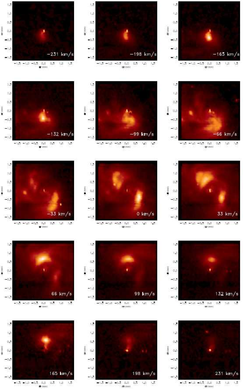
Figure 8 shows slices through the data cube around the H₂ line. The width of the velocity slices is 33 km s^-1, corresponding to one pixel in wavelength direction (i.e. half the spectral resolution $\sigma_{\rm{instr}}$). Material located near the nucleus is present in several consecutive panels, indicating that the material has a high velocity dispersion. In addition there is material that appears in shell-like structures only in one or two bins, hinting towards a lower velocity dispersion. The surface brightness of the H₂  gas seems to be highest along the jet direction for $0\farcs 5<\rm{r}<1\farcs 3$ (see Figure 6). We actually see shell-like structures that might be due to shocked H₂ gas; this hypothesis is supported by the fact that the [Si vi]  and Br$\gamma$  gas distributions fit quite nicely into the shells seen in H₂.

Figure 8.— Velocity channel maps for the molecular gas (H₂ ) at $\lambda$2.121 $\mu$m observed in the K-band. The middle panel shows the flux in the velocity bin that corresponds to the recession velocity of the overall galaxy (532 km s^-1). The other bins slice the cube at blue- and redshifted velocities to this zero position. The width of the velocity slices is 33 km s^-1

Looking at the flux distribution of H₂  (Figure 6), in the radial range $\rm{r}<0\farcs 4$ a elongated structure which might be reminiscent of a disk is visible with a major axis of P.A.=$136\arcdeg$. Ellipse fits to this disk structure give a minor-to-major axis ratio of ${\rm q}\sim 0.67$ which translates to an inclination angle of $\sim 48\arcdeg$ given a circular thin disk configuration. The hypothesis of the central disk structure is also supported by the shape of the velocity dispersion field. Looking at the right panel of Figure 6 we see a disk-like structure with a major-axis position angle of $\sim 140\arcdeg$ inside $\sim 0\farcs 4$.

Drawing on this qualitative description of the H₂  line distribution, and the conjecture that the gas moves in a disk, we model the emission line surface brightness in two parts: an exponential disk that dominates the inner $0\farcs 5$ and a smoothed version of the actually observed H₂  flux distribution resembling the detailed gas morphology in the region outside $0\farcs 5$, where the PSF convolution is less critical. For the black hole mass modeling it is not important to add the second (larger) component, since the inner $<0\farcs 5$ are dominant. Nevertheless we add it to get a better estimate of the influence of the non-symmetric gas distribution on the appearance of the gas velocity field, since part of the small-scale structure in the velocity fields can be reproduced by a patchy gas surface brightness folded into the model (Barth et al., 2001).

We have tested the influence of the parameterization of the exponential disk component on the resulting best-fit black hole mass, and find that a profile that puts $\sim$12% more (less) flux inside the central $0\farcs 5$ (but still fits the observed flux distribution well) results in a black hole mass that is less than 3% lower (higher). This result is in line with the extensive tests on the influence of the surface brightness parameterization carried out by Marconi et al. (2006). In any case, this uncertainty is small compared to other uncertainties that enter the black hole mass measurement, e.g. the inclination angle of the gas disk.

4.4. Tilted-ring model

The kinematics predicted by a flat, or co-planar, thin-disk model must be an oversimplification, as becomes apparent when comparing to the observed data. The twists in the velocity field cannot be reproduced, and the velocity gradient is strictly declining from the peak at $\sim 0\farcs 2$ outwards without being able to resemble the second and third peak at $0\farcs 45$ and $1\farcs 1$ ($\sim 19$pc). We therefore model the kinematics via a tilted-ring model (Begeman, 1987) as it was done before on scales of $r\sim 0\farcm 5$ to $3\arcmin$ by Quillen et al. (1992) and Nicholson et al. (1992) who modeled the CO(2-1) and H$\alpha$ velocity fields in Cen A, respectively. The difference to a coplanar model is that the inclination angle and position angle of the gas disk are a function of radius. The orbits of the gas at each radius remain circular, but neighboring orbits are not necessarily in the same plane. The gas-disk geometry changes from co-planar to warped.

We work in polar coordinates and use discrete radial steps where the model is to be calculated. The model is linearly interpolated between the discrete points on the model grid. The gas disk is made up of concentric rings. Each ring is represented by three parameters: its radius, $R$, inclination angle $i$, and azimuthal angle $\zeta$ (relative to the projected major axis). When projected along the line-of-sight, the rings become ellipses. The flattening, $q$, of the major and minor axes is related to the inclination angle $i$ via $\cos(i)=q$. The flattening defines an ellipse on the sky of ellipticity $\epsilon=1-q$. If the gas is assumed to move on circular orbits along the rings, the projected velocity can be described by the simple cosine form

$$v(R,\zeta)=v_{sys}+v_{c}(R)\sin(i(R))\cos(\zeta(R)),$$ (4)

where $v_{c}(R)$ denotes the circular velocity on a given ring of radius $R$, while $v_{sys}$ gives the systemic velocity of the entire galaxy. This method of expanding the full gas velocity field in a set of tilted rings goes back to the work of Begeman (1987). Here, we are using the method of Krajnović et al. (2006), called kinemetry, to determine the set of ellipses along which the velocity field is best described by equation (4). This method is a generalisation of surface photometry to all moments of the line-of-sight velocity distribution. It performs harmonic expansion of 2D maps of observed kinematic moments (velocity, velocity dispersion, and higher Gauss-Hermite terms) along the best fitting ellipses (either fixed or free to change along the radii). The parameters of the best-fit kinemetry model, using 27 tilted rings, are plotted in Figure 9 and listed in Table 1, while Figure 10 shows the fitted circular velocity map, using these parameters. Note that the parameters of the tilted-ring model vary smoothly with radius, although we do not restrict the kinemetry routine to smooth functions $i(R)$ and $\rm{PA}(R)$. We refer the interested reader to Krajnović et al. (2006) for a detailed description of the kinemetry method.

Figure 9.— Disk parameters of the kinemetry fit to the velocity field as a function of projected radius. The inclination angle $i$ is derived from the flattening $q$ ($i=\arccos(q)$)

Figure 10.— The symmetrized H₂ velocity field (left panel) compared to the best fit kinemetry model (right panel). See Section 4.4 for a description of the kinemetry model. The ellipse shows the flattening of the largest circle

Table 1Parameters of the tilted ring model

R [$\arcsec$]	P.A. [$\arcdeg$]	$q$		i [$\arcdeg$]	$v$ [km  s-1]
0.05	144.0	0.71		45.0	55.
0.10	148.5	0.77		37.6	106.
0.16	152.1	0.79		38.8	112.
0.22	154.8	0.70		42.2	107.
0.27	160.5	0.66		44.5	110.
0.33	165.4	0.56		42.3	110.
0.39	167.8	0.60		44.1	113.
0.45	168.5	0.64		45.7	115.
0.51	168.9	0.67		44.0	109.
0.57	169.0	0.78		39.5	103.
0.63	167.2	0.81		36.1	96.
0.69	165.2	0.82		35.1	89.
0.76	163.5	0.82		34.2	82.
0.82	161.7	0.82		35.2	79.
0.89	159.8	0.80		36.9	76.
0.96	157.0	0.80		36.8	76.
1.03	153.8	0.80		36.2	75.
1.10	151.1	0.80		36.8	75.
1.18	149.3	0.76		39.7	76.
1.26	147.8	0.74		42.5	77.
1.34	146.8	0.69		46.7	80.
1.42	145.1	0.65		48.9	83.
1.51	144.0	0.61		51.6	85.
1.60	142.8	0.58		53.6	87.
1.69	141.6	0.56		55.6	88.
1.79	137.9	0.64		54.6	90.
1.90	134.9	0.58		58.9	89.

5. Results

We now focus on modeling the H₂  gas kinematics in the central $1\arcsec$ ($\sim 17$pc) of NGC 5128 with a warped disk model where the gas orbits in the joint potential of the stars and the central black hole. The central black hole mass as well as the overall inclination angle of the gas disk are varied to find the best-fit to the observed velocity and velocity dispersion maps.

5.1. Structure of the H₂ disk

The rotational velocity field seen in molecular hydrogen shows beautiful symmetry about the center despite the twist that alters the projected orientation of the kinematic major axis by $\pm 14\arcdeg$ about a mean value of $\sim 155\arcdeg$ (see Table 1). Especially for the central values, the orientation of the H₂ gas disk is consistent with an orthogonal disk-jet picture, as the radio jet in Cen A is located at a position angle of $51\arcdeg$ (Tingay et al., 1998).

In addition to the twist in position angle there is a superimposed variation of inclination angle that causes the maximum of the projected rotational velocity to vary by $\pm$ 30 km s^-1 (around a mean value of 90 km s^-1, cf. Table 1). This variation is indeed significant compared to the uncertainty of the velocity which is $\sim\pm$5 km s^-1 (see Section 2.3.

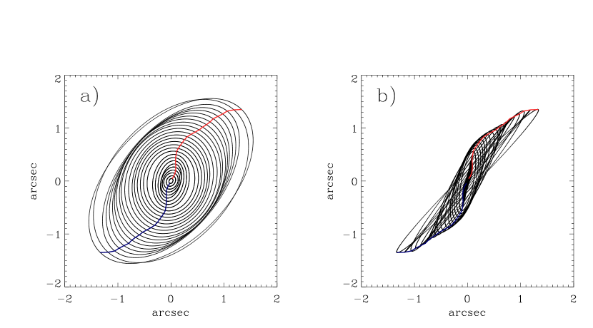
The structure of the gas disk as fitted by the tilted-ring model is presented in Figure 11. For this fit the velocity field was symmetrized using the assumption $v(x,y)=-v(-x,-y)$. The left panel (a) shows the actual kinemetry fit to the symmetrized velocity field. In panel (b) the disk is rotated by 45$\arcdeg$ to an almost edge-on view, to make the warp clearly visible. The position angle twist is indicated by the red and blue lines for the receding and approaching side, respectively.

Figure 11.— Tilted-ring model to describe the nuclear H₂, gas disk seen at (a) the original orientation as fitted by kinemetry and (b) rotated by $45\arcdeg$ to make the warp more visible. The red and blue lines are the line-of-nodes for the receding and approaching side, respectively

Our SINFONI integral field data allow us to constrain the inclination angle of the gas disk very well. Its mean value is $45\arcdeg\pm 7\arcdeg$, which is in very good agreement with the best-fitting inclination angle measured by HN+06 from their NaCo long-slit data ($45\arcdeg$). The inclination angle is also in agreement with the value derived by Hardcastle et al. (2003) from VLA data ($20\arcdeg<i<50\arcdeg$), it is however somewhat smaller than the value from VLBI data derived by Tingay et al. (1998) ($50\arcdeg<i<80\arcdeg$).

The central H₂  gas kinematics are well described by the tilted-ring model. As already stated above, a coplanar disk model would not be able to reproduce the twist in the rotational velocity field and would therefore represent an oversimplification of the kinematic structure. The coplanar disk model can be ruled out at almost 3$\sigma$ confidence level.

The warp of the larger scale disk ($>10\arcsec$) was probably caused by the merger event, that occurred a few times $10^{8}$ years ago (Quillen et al., 1993; Peng et al., 2002). It is not a priori clear whether the warp in the innermost arcsecond is connected to this larger scale warp that creates the prominent appearance of the dust disk in Cen A (Quillen et al., 2006). For the nuclear gas disk on scales $\lesssim 1\farcs 2$ ($\lesssim 20$pc) self-induced warping of the accretion disk (Pringle, 1996) might be the driving mechanism. Our model is not intended to explain the origin of the warp, but is rather meant as a geometric model to resemble the observed velocity field.

5.2. Importance of the inclination angle

The best-fit black hole mass in gas dynamical models depends strongly on the inclination angle assumed for the gas disk model ($\rm{M_{BH}}\varpropto\sin(i)$). Any uncertainty in the disk inclination angle will directly propagate to the uncertainty in the black hole mass.

Our tilted-ring model fitted by kinemetry fixes the overall shape of the gas disk in the model. However, we allow for overall variations in the inclination angle, not to overconstrain the model. That means the position angles for the tilted-rings remain fixed, as well as their relative orientation. While we fix the overall ‘twist’ of the disk a priori, we allow the full dynamical model to re-fit the global inclination. In that way we make use of the geometrical information that is contained in the velocity field (using kinemetry), but at the same time give our dynamical model the freedom to find the best inclination angle given the general assumptions of the model.

5.3. Best-fit model and black hole mass

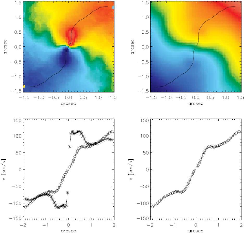
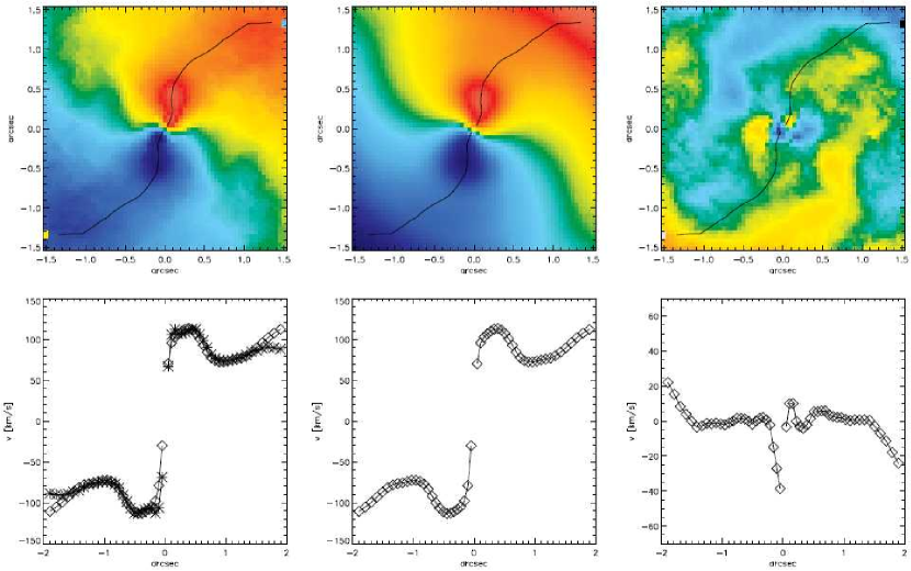
We calculate a grid of possible models for varying disk inclination and central black hole mass to get the set of values that best match the observed data. The best-fitting black hole mass in our tilted-ring model to the H₂  kinematics is $\rm{M_{BH}=4.5^{+1.7}_{-1.0}\times 10^{7}M_{\odot}}$ for a median inclination of $\sim 34\arcdeg\pm 4\arcdeg$ (error bars are given at the 3$\sigma$ level). The best model has a $\chi^{2}$ _min of 8.2. This represents the minimum in the $\Delta$$\chi^{2}$   distribution, shown in Figure 12. The points represent models. The contours were determined by a two-dimensional smoothing spline interpolated from these models and represent $\Delta$$\chi^{2}$   values of 1.0, 4.0, and 9.0. This corresponds to 68.3%, 95.4%, and 99.7% confidence levels for 1 degree of freedom, or 1$\sigma$, 2$\sigma$, and 3$\sigma$ confidence levels, respectively. The associated best-fit model velocity maps are shown in comparison to the data in Figure 13. If we would keep the inclination angle fixed to the mean value of 45$\arcdeg$ given by kinemetry the model is not able to reproduce the overall velocity field. The main deviation between model and data appears for radii larger than $\sim 0\farcs 7$, i.e. outside the radius of influence of the black hole, where the model results in a rotational velocity that is significantly higher than the observed one. The $\chi^{2}$ _min for this “best-fit” model is 16.8 with a best-fit $\rm{M_{BH}\sim 3.0\times 10^{7}M_{\odot}}$. This model is thus ruled out to over 3$\sigma$. The entire velocity field is better reproduced by a disk at lower inclination (i.e. more face-on) plus a higher black hole mass that makes up for the decrease in velocity inside the radius of influence of the black hole.

Figure 14 shows a comparison of the model and the data for the case of no central point mass. Here, the gravitational potential is made up only by the stars. The mass-to-light ratio is 0.72 $\rm{M/L_{\odot,K}}$ (HN+06). It is obvious that this is no good fit in the central $0\farcs 5\times 0\farcs 5$. The modeled rotation only catches up with the data outside $\sim 1\farcs 0$, where the stars clearly dominate the gravitational potential. The case for no black hole is excluded to very high significance (over 8$\sigma$).

There are various factors that influence the black hole mass estimate in our dynamical model and we have done a substantial number of tests to scrutinize their impact on the best-fit result. As mentioned in Section 5.1 the assumed geometry of the disk (warped vs. flat) has a small influence on the black hole mass. The same holds true for the parameterization of the surface brightness. We modeled the kinematics for three different parameterizations of the disk’s surface brightness profile, with all three being a reasonable fit to the data. We found that the black hole mass does change by less than 3% depending on the assumed surface brightness profile of the inner gas disk. This result is in agreement with the detailed analysis of Marconi et al. (2006).

Obviously, also the contribution of the stellar potential to the total gravitational potential influences the resulting best-fit black hole mass. We used the two extreme values 0.72 $\rm{M/L_{\odot,K}}$ and 0.53 $\rm{M/L_{\odot,K}}$ derived by Silge et al. (2005) through stellar dynamical models at inclination angles 90$\arcdeg$ and 45$\arcdeg$, respectively (the value for 20$\arcdeg$ is 0.68 $\rm{M/L_{\odot,K}}$ and lies in between these two). Using 0.53 $\rm{M/L_{\odot,K}}$, the best-fitting black hole mass increases by $\sim 8\%$ compared to the best-fit value of $\rm{M_{BH}=4.5\times 10^{7}M_{\odot}}$ (for 0.72 $\rm\,{M/L_{\odot,K}}$). The uncertainty introduced by the inclination angle is much larger than this, which is reflected by the fairly large uncertainty limits on our black hole mass measurement.

Figure 12.— Constraining the mass of the central black hole: The Figure indicates the grid of models (in black hole mass, M_BH, and disk inclination) that was calculated, and the contours show $\Delta$$\chi^{2}$   in the vicinity of the best fit dynamical models for matching the H₂, kinematics. The minimum $\chi^{2}$   model is at a $\rm{M_{BH}\sim 4.5\times 10^{7}M_{\odot}}$ and a median disk inclination of 34$\arcdeg$. The contours indicate the 1$\sigma$, 2$\sigma$, and 3$\sigma$ confidence levels, respectively (see text for details)

Figure 13.— Velocity field of the best-fitting dynamical model (center, top), with a black hole mass of $\rm{4.5\times 10^{7}M_{\odot}}$ and a median disk inclination of 34$\arcdeg$, in comparison to the data (top left). The velocity residual (data-model) is shown in the right panel. The velocity curves in the bottom panels are extracted along the line-of-nodes (overplotted to the velocity maps), and represent the peak velocity curves. The diamonds correspond to the model velocity curve while the crosses correspond to the data. A mismatch in the data and model most prominent beyond r$\lesssim-1\farcs 7$ is likely due to the fact that the inclination angle of the modeled gas disk is not well represented in the outermost parts. This has no impact on the derived black hole mass

Figure 14.— Kinematic evidence for a central black hole: The top panels compare the observed symmetrized H₂ velocity field (left) to a velocity field model for the case of zero black hole mass with only a stellar potential, derived by HN+06 (right). The bottom panels show the velocity curves extracted along the line-of-nodes (indicated in the top panels). Obviously, this model is not a good fit to the data in the central $0\farcs 8\times 0\farcs 8$. Only beyond $1\farcs 0$ are the model velocity curve (diamonds) in reasonable agreement with the data (crosses)

5.4. Asymmetries in the H₂ velocity field

The overall shape of the H₂  velocity field appears to be point-symmetric about the position of the AGN (the peak in the K-band continuum which is coincident with the peak in the H₂ surface brightness). This symmetry is proven and illustrated by the smooth kinemetry fit.

However, taking a closer look at the peak velocities in the field, it is striking, that the peak velocity in the blue dip at $(x,y)=(-0\farcs 2,-0\farcs 5)$ exceeds the one in the corresponding red peak ($(x,y)=(0\farcs 2,0\farcs 5)$) by $\sim 30$ km s^-1 (corresponding to $\sim 30\%$ of the peak velocity).

The reason for this asymmetry is not merely an overall velocity shift, since that would affect the whole field. This can be ruled out by the fact that the absolute values of the velocities are in excellent agreement for radii larger than $\sim 0\farcs 8$.

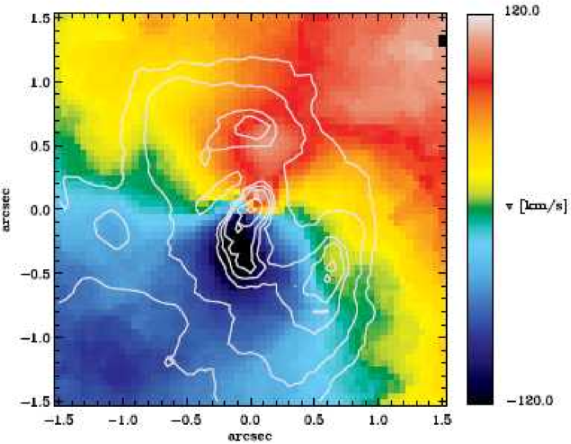
It is instructive to overplot the iso-flux contours to the velocity field (see Figure 15), since one clearly sees that the asymmetry in the velocity field is also present in the flux distribution. This leads us to speculate that the gas density is not the same throughout the disk, as a higher density leads to a higher flux. The density might be increased by gas that is streaming towards the central disk. This might be of similar origin as the non-rotational motions observed in [Fe ii], Br$\gamma$, and [Si vi]  but is not as obvious in molecular hydrogen. The asymmetry is also present in the Br$\gamma$  and [Si vi]  velocity maps, being strongest in [Si vi]. What we observe here, might be the fueling process of the nuclear disk.

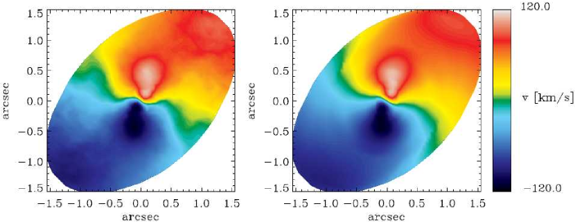
Our gas dynamical model is by construction symmetric, and therefore not able to reproduce asymmetries in the velocity structure. For determining the best-fit black hole mass, we have minimized the difference of the symmetric model to the asymmetric data, looking for the best compromise. After having gained the best-fit model (to the original data) we are free to compare this to a symmetrized version of the H₂ velocity field, $v_{\rm{sym}}(x,y)=(v(x,y)-v(-x,-y))/2$. The agreement, as shown in Figure 16, is astonishing.

Figure 15.— The H₂ surface brightness contours are overplotted to the H₂ velocity map. The velocity field is asymmetric in the sense that the blue dip is of larger amplitude (in the center-of-mass system) than the red peak. This asymmetry is also seen in the flux contours, but such asymmetries are not captured by our model

Figure 16.— The symmetrized velocity map (top left) in comparison to the model ($M_{BH}=\rm{4.5\times 10^{7}M_{\odot}}$ and $<i>=34\arcdeg$ - top middle panel). The residual (data-model) is shown in the right panel. The velocity curves in the bottom panels are extracted along the line-of-nodes (overplotted to the velocity maps), and therefore represent the peak velocity curves. The diamonds correspond to the model velocity curve while the crosses correspond to the data. The agreement is very good along the line-of-nodes. The mismatch in data and model for radii beyond r$\sim\pm 1\farcs 7$ is likely due to the fact that the inclination angle of the modeled gas disk is not well represented in the outermost parts. This has no impact on the derived black hole mass

6. Discussion

The high resolution 2D data have now reached a quality that the existence of a central black hole (or compact mass) can be demonstrated, and its mass be estimated, even without a sophisticated model, e.g. by just using the concept of the radius of influence of the black hole, r_BH. This is the region where the mass of the enclosed stars equals the mass of the supermassive black hole:

$$\rm{r_{BH}=\frac{GM_{BH}}{\sigma^{2}_{*}}},$$ (5)

where $\rm{M_{BH}}$ is the mass of the black hole, G is the gravitational constant and $\sigma_{*}$ is the velocity dispersion of the stellar spheroid. In the velocity field, this is the point of minimum rotation, where the black hole stops to dominate the gravitational potential, before the stars (with their rising rotation curve) take over. For our H₂  velocity this is at $\sim 0\farcs 8$ as seen in Figure 16 (left panel). For Cen A we have the following numbers: $\sigma_{*}=138$ km s^-1 (Silge et al., 2005), at D=3.5 Mpc, $\rm{r_{BH}}=0\farcs 8\pm 0\farcs 1=$ 13.2 pc$\pm 1.7$ pc, and therefore we get $\rm{M_{BH}=(6.0\pm 0.7)\times 10^{7}\,M_{\odot}}$.

The observed radius of minimum rotation is independent of the inclination and so this simple concept provides a nice check on the black hole mass derived via dynamical modeling. Given the excellent spatial resolution of our AO-assisted data (FWHM${}_{\rm{core}}=0\farcs 12$ and FWHM${}_{halo}=0\farcs 30$) the observed radius of influence of the black hole is well beyond the radius where PSF effects start significantly affecting the derived velocity curve.

The best-fit black hole mass derived through modeling of the H₂ kinematics, $\rm{M_{BH}=(4.5^{+1.7}_{-1.0})\times 10^{7}M_{\odot}}$ at $i=34\arcdeg\pm 4\arcdeg$, is in good agreement with the mass derived by HN+06 ($\rm{(6.1^{+0.6}_{-0.8})\times 10^{7}M_{\odot}}$ at $i=45\arcdeg$) using high spatial resolution kinematics of [Fe ii]  derived from AO-assisted NaCo long slit data (FWHM$=0\farcs 11$). The dynamical model they used is in principle identical to the one described above, except the fact that we cover the velocity field in two dimensions and they modeled only four slit positions. Moreover, they did not include the disk inclination angle as a free parameter, which is the main reason for their smaller error bars. Concerning the disk geometry, HN+06 excluded disk inclination angles below $45\arcdeg$ due to the jet inclination derived by Tingay et al. (1998), who give $50\arcdeg<i<80\arcdeg$. However, following the analysis of Hardcastle et al. (2003), who use jet-counterjet ratios and apparent motions in the jet, the jet inclination is most likely in the range $20\arcdeg<i<50\arcdeg$. HN+06 state that if they were to allow an inclination angle of $i=25\arcdeg$ with respect to the line-of-sight, their best-fit black hole mass is $\sim 1.2\times 10^{8}M_{\odot}$. This is significantly larger than the value we measure. But one has to take into account, that the modeled gas species are not the same for the two studies. While the molecular gas has a well-ordered rotation field, the 2D velocity field of [Fe ii]  (Fig. 5) clearly exhibits two components: inflow and rotation. This superposition could not be seen in the long-slit data and was not accounted for in the model of HN+06. They modeled the total [Fe ii]  kinematics under the assumption of gas rotating in a flat, thin disk.

6.1. Comparison to previous gas dynamical models

The agreement of our modeling results with the recent analysis of Krajnović et al. (2007) is comfortable: they modeled integral-field Pa$\beta$ kinematics and derived $\rm{M_{BH}=8.25^{+2.25}_{-4.25}\times 10^{7}M_{\odot}}$ at $i=25\arcdeg$ (where the error bars are also at the 3$\sigma$ confidence level). The resolution of their seeing limited data is $0\farcs 5-0\farcs 6$, i.e. a factor of $\sim 4-5$ larger than ours, but good enough to resolve the radius of influence of the black hole in Cen A. Again, the somewhat larger black hole mass value might be attributed to the fact that (Krajnović et al., 2007) model the kinematics of the ionized gas species Pa$\beta$, which might also be affected by non-gravitational motions.

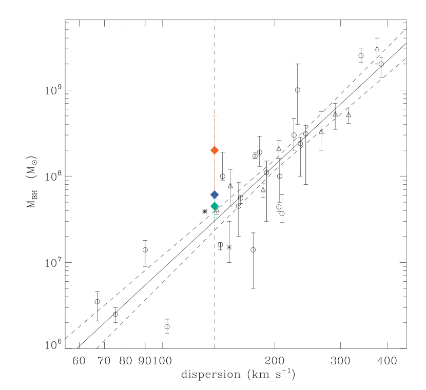
This decrease in black hole mass compared to recent dynamical measurements of ionized gas by Marconi et al. (2001) (M${}_{\rm{BH}}=2.0^{+3.0}_{-1.4}\times 10^{8}\rm{M}_{\odot}$), Häring-Neumayer et al. (2006) (M${}_{\rm{BH}}=6.1^{+0.6}_{-0.8}\times 10^{7}\rm{M}_{\odot}$), Marconi et al. (2006) (M${}_{\rm{BH}}=6.5^{+0.7}_{-0.7}\times 10^{7}\rm{M}_{\odot}$), and Krajnović et al. (2007) ($\rm{M_{BH}=8.25^{+2.25}_{-4.25}\times 10^{7}M_{\odot}}$) brings Centaurus A in agreement with the M_BH-$\rm{\sigma}$ relation (Ferrarese & Merritt, 2000; Gebhardt et al., 2000) (see Fig. 17). All previous gas dynamical studies were based on ionized gas species, which are most probably all influenced by Cen A’s jet, and are no good tracers of the gravitational potential in the innermost arcsecond. One of the main advantages of our high resolution two-dimensional data is to be able to reveal the jet’s influence and to choose the appropriate gas species for the dynamical model.

Figure 17.— Black hole mass (M_BH) vs. stellar velocity dispersion along with the best fit correlation as compiled by Tremaine et al. (2002). Mass measurements based on stellar kinematics are denoted by circles, on gas kinematics by triangles, and on maser kinematics by asterisks. Filled diamonds denote mass measurements of Cen A’s black hole by Marconi et al. (2001) (red), HN+06 (blue), and this work (green). The dashed lines show the 1$\sigma$ confidence levels on the best-fit correlation. Our high resolution two-dimensional kinematic maps and dynamical modeling bring Cen A in full agreement with the M_BH-$\rm{\sigma}$ relation

6.2. Comparison to stellar dynamical models

Using stellar kinematics (v, $\sigma$, $h_{3}$, and $h_{4}$) derived from Gemini GNIRS data along two slit-positions with seeing-limited resolution of $0\farcs 4$ to $0\farcs 65$ Silge et al. (2005) derive a best-fit black hole mass of $2.4^{+0.3}_{-0.2}\times 10^{8}M_{\odot}$ for an edge-on model, $1.8^{+0.4}_{-0.4}\times 10^{8}M_{\odot}$ for a model with i=45$\arcdeg$, and $1.5^{+0.3}_{-0.2}\times 10^{8}M_{\odot}$ for a model with an inclination of 20$\arcdeg$ (note that theses error bars are at the 1$\sigma$ confidence level).

Using integral-field stellar kinematics (v, $\sigma$, $h_{3}$, and $h_{4}$) derived from the same SINFONI data set used for the underlying gas dynamical study, Cappellari et al. (in prep.) get a best-fit black hole mass of $5\pm 3\times 10^{7}M_{\odot}$ (3$\sigma$ error bars). This value is more than a factor of $\sim 3$ lower than the value derived by Silge et al. (2005), it is, however, in full agreement with the gas dynamical measurement presented in the current paper.

This is an important result for the general comparison of stellar and gas kinematical modeling of black hole masses. Up to now only a couple of these comparative cases have been investigated and in half of the cases with negative results (e.g. Cappellari et al., 2002b; Shapiro et al., 2006).

This is the first case where the modeling techniques can be tested on stellar and gas kinematical data extracted from the same complete data set. The fact that we deal with integral-field kinematics allows the constraints on the black hole mass to be significantly tightened compared to long-slit observations. The excellent agreement between gas and stellar dynamical modeling results thus provides stringent evidence for the reliability of both techniques.

7. Conclusions

This work presents observations of the nearby active elliptical galaxy NGC 5128 (Cen A) with the adaptive-optics assisted integral field spectrograph SINFONI at the VLT. Our K-band data used to measure the black hole mass in Cen A from emission line kinematics have a spatial resolution of $0\farcs 12$ and an estimated Strehl ratio of $\sim 17\%$. The field of view is $3\arcsec\times 3\arcsec$.
In our H- and K-band data we detect the following emission lines: [Fe ii], [Si vi], He i, Br$\gamma$, [Ca viii], and several vibrational transitions of molecular hydrogen, H₂  (the strongest is 1-0 S(1) at 2.12$\mu$m). The main results of our analysis are:

• Analysing the velocity fields of [Si vi], Br$\gamma$, [Fe ii], and the strongest H₂  line, we find that the surface brightness and also the motion of the gas species is increasingly influenced (or produced) by the jet when going from low to high excitation lines. The velocity fields of [Si vi], Br$\gamma$, and [Fe ii]  clearly exhibit two components: 1) rotational motion at a major angle of $\sim 150\arcdeg$, consistent with an orthogonal disk-jet picture, and 2) non-rotational motion along the direction of the jet, that is consistent with a back-flow of gas along the side of the jet’s cocoon. This non-rotational component is strongest for [Si vi].

• The surface brightness of H₂  shows an indication of a central gas disk at a position angle of P.A.$\sim 136\arcdeg$ and a minor-to-major axis ratio of 0.67. The bright spots NE and SW of the nuclear disk remind of the lobes seen on much larger scales in jet-gas interactions.

• The overall velocity field of H₂  shows beautiful point-symmetry about the unresolved nucleus. However, the H₂  peak velocities are asymmetric inside the central $0\farcs 7$. This asymmetry is also seen in the surface brightness map of H₂, and might be explained by denser gas that leads to an increase in flux. The density could be increased by gas that is streaming towards the central disk. This might be similar to the non-rotational motions observed in [Fe ii], Br$\gamma$, and [Si vi]  but is not as obvious in molecular hydrogen. It is possible that we see the fueling process of the nuclear disk.
  Another influence of the jet on the velocity field might be the twists in the zero velocity curve (at the positions where the lobes appear in the surface brightness map of H₂). The rotational major axis (line-of-nodes) runs from SE to NW, with the SE side blue- and the NW side redshifted with respect to the nucleus. It follows the shape of an “S”. The velocity field is reminiscent of a warped disk. Judging from the smooth velocity field of the H₂  gas, the major part of molecular hydrogen is well settled in the total gravitational potential $\Phi_{\star}+\Phi_{\rm{BH}}$, and is therefore a good tracer of the central black hole mass.

• Under the assumption of gas moving on circular orbits, we fit the geometry of the gas disk with a set of tilted rings, using kinemetry (Krajnović et al., 2006). The mean P.A. is 155$\arcdeg$ with twists of $\pm 14\arcdeg$. The median inclination angle is $\sim 45\arcdeg\pm 12\arcdeg$.

• We construct a tilted-ring model for the central H₂  gas motions, in the combined potential of the stars and the black hole. We account for the velocity dispersion via a pressure term in the isotropic, axisymmetric Jeans’ equation. The geometry of the disk is fixed via the kinemetry fit to the velocity field, but we allow the overall inclination angle to vary. Our best-fit model has a mean inclination angle of $34\arcdeg\pm 4\arcdeg$, and a black hole mass of $\rm{M_{BH}=(4.5^{+1.7}_{-1.0})\times 10^{7}M_{\odot}}$. We find that the inclination angle, derived through the kinemetry fit is not able to reproduce the overall velocity field. We conclude that the optimal choice would be to simultaneously fit the disk geometry and the black hole mass.

  As our dynamical model is by construction symmetric about the center, it fails to reproduce the asymmetry in the H₂  data. When symmetrising the velocity field, the agreement of data and model is excellent.

• Our black hole mass measurement is somewhat smaller but still consistent with previous gas measurements using ionized gas species. It is substantially smaller than the stellar dynamical model of Silge et al. (2005). However, it is in perfect agreement with the stellar dynamical measurement of Cappellari et al. (in prep.) who extract the stellar kinematics from the same SINFONI data set.

• Our black hole mass determination brings Cen A in agreement with the $\rm{M_{BH}-\sigma}$ relation (Ferrarese & Merritt, 2000; Gebhardt et al., 2000).

References

- Barth et al. (2001) Barth, A. J., Sarzi, M., Rix, H.-W., Ho, L. C., Filippenko, A. V., & Sargent, W. L. W. 2001, ApJ, 555, 685
- Begeman (1987) Begeman, K. G. 1987, Ph.D. Thesis, Groningen University
- Bertola et al. (1998) Bertola, F., Cappellari, M., Funes, J. G., Corsini, E. M., Pizzella, A., & Vega Beltrán, J. C. 1998, ApJ, 509, L93
- Binney & Tremaine (1987) Binney, J., & Tremaine, S. 1987, Princeton, NJ, Princeton University Press, 1987, 747 p.
- Bonnet et al. (2003) Bonnet, H., et al. 2003, Proc. SPIE, 4839, 329
- Bonnet et al. (2004) Bonnet, H. et al. 2004, The ESO Messenger 117, 17
- Cappellari et al. (2002b) Cappellari, M., Verolme, E. K., van der Marel, R. P., Kleijn, G. A. V., Illingworth, G. D., Franx, M., Carollo, C. M., & de Zeeuw, P. T. 2002b, ApJ, 578, 787
- Cappellari (2002a) Cappellari, M. 2002a, MNRAS, 333, 400
- Cappellari & Emsellem (2004) Cappellari, M. & Emsellem, E. 2004, PASP, 116, 138
- Carilli et al. (1988) Carilli, C. L., Perley, R. A., & Dreher, J. H. 1988, ApJ, 334, L73
- Clarke et al. (1992) Clarke, D. A., Burns, J. O., & Norman, M. L. 1992, ApJ, 395, 444
- Eisenhauer et al. (2003a) Eisenhauer, F., et al. 2003a, Proc. SPIE, 4841, 1548
- Eisenhauer et al. (2003b) Eisenhauer, F., et al. 2003b, The Messenger, 113, 17
- Emsellem, Monnet, & Bacon (1994) Emsellem, E., Monnet, G., & Bacon, R. 1994, A&A, 285, 723
- Evans et al. (2004) Evans, D. A., Kraft, R. P., Worrall, D. M., Hardcastle, M. J., Jones, C., Forman, W. R., & Murray, S. S. 2004, ApJ, 612, 786
- Ferrarese & Merritt (2000) Ferrarese, L., & Merritt, D. 2000, ApJ, 539, L9
- Ferrarese & Ford (2005) Ferrarese, L., & Ford, H. 2005, Space Science Reviews, 116, 523
- Ferrarese et al. (2007) Ferrarese, L., Mould, J. R., Stetson, P. B., Tonry, J. L., Blakeslee, J. P., & Ajhar, E. A. 2007, ApJ, 654, 186
- Gebhardt et al. (2000) Gebhardt, K., et al. 2000, ApJ, 539, L13
- Gerhard (1993) Gerhard, O. E. 1993, MNRAS, 265, 213
- Grandi et al. (2003) Grandi, P., et al. 2003, ApJ, 593, 160
- Häring & Rix (2004) Häring, N., & Rix, H.-W. 2004, ApJ, 604, L89
- Häring-Neumayer et al. (2006) N. Häring-Neumayer, M. Cappellari, H.-W. Rix, M. Hartung, M. A. Prieto, K. Meisenheimer, R. Lenzen, 2006, ApJ, 643, 226
- Hardcastle et al. (2003) Hardcastle, M. J., Worrall, D. M., Kraft, R. P., Forman, W. R., Jones, C., & Murray, S. S. 2003, ApJ, 593, 169
- Israel et al. (1990) Israel, F. P., van Dishoeck, E. F., Baas, F., Koornneef, J., Black, J. H., & de Graauw, T. 1990, A&A, 227, 342
- Israel (1998) Israel, F. P. 1998, A&A Rev., 8, 237
- Jones et al. (1996) Jones, D. L., et al. 1996, ApJ, 466, L63
- Kormendy & Richstone (1995) Kormendy, J., & Richstone, D. 1995, ARA&A, 33, 581
- Krajnović et al. (2006) Krajnović, D., Cappellari, M., de Zeeuw, P. T., & Copin, Y. 2006, MNRAS, 366, 787
- Krajnović et al. (2007) Krajnović, D., Sharp, R., & Thatte, N. 2007, MNRAS, 374, 385
- Krause (2005) Krause, M. 2005, A&A, 431, 45
- Macchetto et al. (1997) Macchetto, F., Marconi, A., Axon, D. J., Capetti, A., Sparks, W., & Crane, P. 1997, ApJ, 489, 579
- Marconi et al. (2001) Marconi, A., Capetti, A., Axon, D. J., Koekemoer, A., Macchetto, D., & Schreier, E. J. 2001, ApJ, 549, 915
- Marconi & Hunt (2003) Marconi, A., & Hunt, L. K. 2003, ApJ, 589, L21
- Marconi et al. (2006) Marconi, A., Pastorini, G., Pacini, F., Axon, D. J., Capetti, A., Macchetto, D., Koekemoer, A. M., & Schreier, E. J. 2006, A&A, 448, 921
- Nicholson et al. (1992) Nicholson, R. A., Bland-Hawthorn, J., & Taylor, K. 1992, ApJ, 387, 503
- Peng et al. (2002) Peng, E. W., Ford, H. C., Freeman, K. C., & White, R. L. 2002, AJ, 124, 3144
- Pringle (1996) Pringle, J. E. 1996, MNRAS, 281, 357
- Quillen et al. (1992) Quillen, A. C., de Zeeuw, P. T., Phinney, E. S., & Phillips, T. G. 1992, ApJ, 391, 121
- Quillen et al. (1993) Quillen, A. C., Graham, J. R., & Frogel, J. A. 1993, ApJ, 412, 550
- Quillen et al. (2006) Quillen, A. C., Brookes, M. H., Keene, J., Stern, D., Lawrence, C. R., & Werner, M. W. 2006, ApJ, 645, 1092
- Quillen et al. (2006) Quillen, A. C., Bland-Hawthorn, J., Brookes, M. H., Werner, M. W., Smith, J. D., Stern, D., Keene, J., & Lawrence, C. R. 2006, ApJ, 641, L29
- Reipurth et al. (2002) Reipurth, B., Heathcote, S., Morse, J., Hartigan, P., & Bally, J. 2002, AJ, 123, 362
- Rejkuba (2004) Rejkuba, M. 2004, A&A, 413, 903
- Schreier et al. (1998) Schreier, E. J., et al. 1998, ApJ, 499, L143
- Shapiro et al. (2006) Shapiro, K. L., Cappellari, M., de Zeeuw, T., McDermid, R. M., Gebhardt, K., van den Bosch, R. C. E., & Statler, T. S. 2006, MNRAS, 370, 559
- Schoenmakers et al. (1997) Schoenmakers, R. H. M., Franx, M., & de Zeeuw, P. T. 1997, MNRAS, 292, 349
- Silge et al. (2005) Silge, J. D., Gebhardt, K., Bergmann, M., & Richstone, D. 2005, AJ, 130, 406
- Taylor et al. (1992) Taylor, D., Dyson, J. E., & Axon, D. J. 1992, MNRAS, 255, 351
- Tingay et al. (1998) Tingay, S. J., et al. 1998, AJ, 115, 960
- Tonry et al. (2001) Tonry, J. L., Dressler, A., Blakeslee, J. P., Ajhar, E. A., Fletcher, A. B., Luppino, G. A., Metzger, M. R., & Moore, C. B. 2001, ApJ, 546, 681
- Tremaine et al. (2002) Tremaine, S., et al. 2002, ApJ, 574, 740
- van der Marel & Franx (1993) van der Marel, R. P., & Franx, M. 1993, ApJ, 407, 525
- van der Marel & van den Bosch (1998) van der Marel, R. P., & van den Bosch, F. C. 1998, AJ, 116, 2220
- Verdoes Kleijn et al. (2002) Verdoes Kleijn, G. A., van der Marel, R. P., de Zeeuw, P. T., Noel-Storr, J., & Baum, S. A. 2002, AJ, 124, 2524