Self-organized escape of oscillator chains in nonlinear potentials

Abstract

We present the noise free escape of a chain of linearly interacting units from a metastable state over a cubic on-site potential barrier. The underlying dynamics is conservative and purely deterministic. The mutual interplay between nonlinearity and harmonic interactions causes an initially uniform lattice state to become unstable, leading to an energy redistribution with strong localization. As a result a spontaneously emerging localized mode grows into a critical nucleus. By surpassing this transition state, the nonlinear chain manages a self-organized, deterministic barrier crossing. Most strikingly, these noise-free, collective nonlinear escape events proceed generally by far faster than transitions assisted by thermal noise when the ratio between the average energy supplied per unit in the chain and the potential barrier energy assumes small values.

I Introduction

The cornerstone work by Kramers (for a comprehensive review see Ref. RMP ) has instigated an ever ongoing interest in the dynamics of escape processes of single particles, of coupled degrees of freedom or of small chains of coupled objects out of metastable states. In undergoing an escape the objects considered manage to overcome an energetic barrier, separating the local potential minimum from a neighboring attracting domain.

Stochastic—i.e., noise-assisted—escape is the predominant phenomenon being studied in statistical physics. Then, the system energy fluctuates while permanently interacting with a thermal bath. This causes dissipation and local energy fluctuations and the process is conditioned on the creation of a rare optimal fluctuation which in turn triggers an escape RMP . In other words, an optimal fluctuation transfers sufficient energy to the chain so that the latter statistically overcomes the energetic bottleneck. Characteristic time-scales of such a process are determined by the calculation of corresponding rates of escape out of the domain of attraction. In this realm, many extensions of Kramers escape theory and of first passage time problems in over- and underdamped versions have been widely investigated RMP ; JSPHa . Early generalizations to multi-dimensional systems date back to the late $1960$’s Langer . This method, nowadays, is commonly utilized in biophysical contexts and for a great many applications occurring in physics and chemistry Sung -BM .

With this work we present a different scenario of a possible exit from a metastable domain of attraction which has recently been put forward in Ref. EPL . The model we shall study is a purely deterministic dynamics of a linearly coupled chain of nonlinear oscillators. Put differently, no additional coupling to a thermal bath promotes the escape. Henceforth, dissipation vanishes as well within this set up. The underlying mechanism to create an escape is caused solely by the strongly nonlinear Hamiltonian deterministic dynamics.

We explore macroscopic discrete, coupled nonlinear oscillator chains with up to $1000$ links. These may appear as realistic models in mechanical and electrical systems, in various biophysical contexts, in neuroscience, or in networks of coupled superconductors, to name but a few neuro -breathers . A deterministic escape in the absence of noise is particularly important in the case of low temperatures when activated escape becomes far too slow. Also the case of many coupled nonlinear units in the presence of non-thermal intrinsic noise that scales inversely with the square root of the system size then calls, in the limit of large system sizes, for a deterministic nonlinear escape scenario.

In the nonlinear regime an initially, almost homogeneous chain is able to generate spontaneous structural modulations. This process proceeds in a self-organized manner. More specifically, due to the modulational instability, unstable growing nonlinear modes give rise to the formation of coherent structures Remoissenet such that the originally uniformly distributed energy becomes concentrated to a few degrees of freedom. With regard to nonlinear localization phenomena intrinsic localized modes or discrete breathers, such as time-periodic and spatially localized solutions of nonlinear lattice systems, have turned out to present the archetype of localized excitations in numerous physical situations MacKay -Josephson .

An escape is related to a crossing of a saddle point in configuration space, corresponding to a bottleneck RMP or a transition state. The latter is associated with an activation energy $E_{act}$ to be concentrated in the critical localized mode. We will show that the critical localized mode can be reached in the microcanonical situation spontaneously EPL . Thus, we encounter a self-organized creation of the transition state which is in clear contrast to noise activated escape. In particular, we demonstrate that intrinsic nonlinear effects on a long discrete chain of $N$ units induce a transition over an energetic barrier by enhancing one, or several localized breather states Flach -breathers . Due to this mechanism the initially almost uniformly distributed energy is dynamically concentrated by use of an internal redistribution; no assistance of energy exchange with a thermal bath is thus needed. We show as well that the nonlinear mechanism of energy localization may promote a faster escape dynamics as compared to the noise-assisted situation where the system experiences an enduring stochastic forcing.

The paper is organized as follows: In the next section we introduce the model of the coupled oscillator chain and discuss in Sec. III the modulational instability as the localization mechanism. In Sec. IV we proceed by focusing our interest on the low-energy modes corresponding to nearly equilibrium states of the lattice chain. The properties of localization induced by the dynamical formation of breather arrays are explored. Concerning the escape itself, special attention is paid to the passage of lattice states through a critical localized mode (transition state) in Sec. V. Subsequently, in Sec. VII we demonstrate that the rate of escape may be crucially affected by the coupling strength. In Sec. VI the escape rates obtained under microcanonical conditions are compared with those found for thermally activated barrier crossings. In this context we assume not only flat-state initial preparations of the microcanonical system but also random chain configurations with a fairly broad distribution of the coordinates and/or momenta. In Sec. VIII we deal with the influence of the chain length on the escape process. We conclude with a summary of our results.

II Coupled oscillator chain model

We study a one-dimensional lattice of coupled nonlinear oscillators. Throughout the following we shall work with dimensionless parameters, as obtained after appropriate scaling of the corresponding physical quantities. The coordinate $q$ of each individual oscillator of mass unity evolves in a cubic, single well on-site potential of the form

$$U(q)=\frac{\omega_{0}^{2}}{2}q^{2}-\frac{a}{3}q^{3}\,.$$ (1)

This potential possesses a metastable equilibrium at $q_{min}=0$, corresponding to the rest energy $E_{min}=0$ and the maximum is located at $q_{max}=\omega_{0}^{2}/a$ with energy $E_{max}\equiv\Delta E=\omega_{0}^{6}/(6a^{2})$. Thus, in order for particles to escape from the potential well of depth $\Delta E$ over the energy barrier and subsequently into the range $q>q_{max}$ a sufficient amount of energy has to be supplied.

The Hamiltonian of the one-dimensional coupled nonlinear oscillator chain is given by

$$H=\sum_{n=1}^{N}\,\left\{\,\frac{p_{n}^{2}}{2}\,+\,U(q_{n})\,\right\}+\,\frac{\kappa}{2}\,\sum_{n=1}^{N}\,\left[\,q_{n+1}-q_{n}\,\right]^{2}\,.$$ (2)

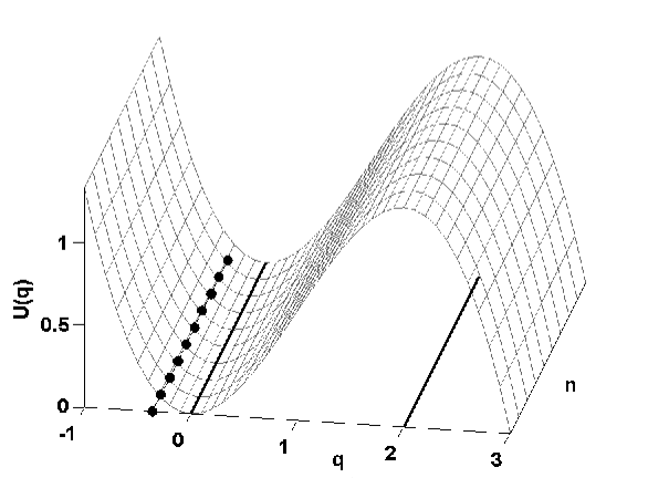
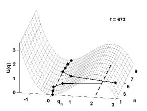
The coordinates $q_{n}(t)$ quantify the displacement of the oscillator in the local on-site potential $U$ at lattice site $n$ (see Fig. 1), and $p_{n}(t)$ denotes the corresponding canonically conjugate momentum. The oscillators, also referred to as ”units”, are coupled linearly to their neighbors with interaction strength $\kappa$.

Figure 1: Potential barrier landscape with a chain positioned at the bottom. The parameter values are $a=1$ and $\omega_{0}^{2}=2$.

The equations of motion derived from the Hamiltonian given in Eq. (2) then read:

$$\frac{d^{2}q_{n}}{dt^{2}}\,+\,\omega_{0}^{2}q_{n}-aq_{n}^{2}-\kappa\,\left[\,q_{n+1}+q_{n-1}-2q_{n}\,\right]=0\,\,.$$ (3)

Throughout this work we use periodic boundary conditions according to $q_{1}(t)=q_{N+1}(t)$. Note that in Eq. (3) the nonlinearity is solely contained in the local force term.

For a setup with interacting strength $\kappa$ the barrier height can be estimated by assuming that only one unit of the chain is elongated, which yields a value $\Delta E_{\kappa}=(\omega_{0}^{2}+2\kappa)^{3}/(6a^{2})$. Hence, compared to the isolated unit, a unit coupled to its neighbors experiences an increase of the barrier height.

For sufficiently small energy per unit of all chain members as compared to the potential barrier, a linear regime with $a=0$ holds true in the considered potential (1), yielding oscillatory solutions in phase space such that the elongations are restricted to the neighborhood of the potential bottom. The corresponding linearized system

$$\delta\ddot{q}_{n}+\omega_{0}^{2}{\delta{q}}_{n}-\kappa\,\left[\,{\delta{q}}_{n+1}+{\delta{q}}_{n-1}-2{\delta{q}}_{n}\right]=0\,,$$ (4)

possesses exact plane-wave solutions (phonons)

$${\delta{q}}_{n}(t)={{u}_{0}}\exp[i(k\,n-\omega\,t)]+c.c.\,,$$ (5)

The wave number $k=2\pi m/N$, with integer $m\in[-N/2,N/2]$, and the frequency $\omega$ are related by the dispersion relation

$$\omega^{2}=\omega_{0}^{2}+4\kappa\,\sin^{2}\left(\frac{k}{2}\right)\,.$$ (6)

This expression determines the frequency of linear oscillations in the phonon band with $k\in[-\pi,\pi]$.

The superposition of phonon modes causes oscillatory states wherein distinguished units may temporarily accumulate energies that are comparable to the barrier energy. However, in a harmonic potential with $a=0$ these states are highly unlikely. If at all, they occur at a time scale comparable to the Poincaré recurrence time of the system.

Nonetheless, utilizing nonlinear effects with $a>0$, an initial state near the metastable minimum is structurally unstable which mobilizes structural transition of the chain such that a transition state is adopted. This mechanism will be elaborated on in the next section.

III Modulational instability

It is well established that the formation of localized excitations in nonlinear systems can be caused by a modulational instability Kivshar92 -Peyrard98 . This mechanism initiates an instability of an initial plane-wave when small perturbations of non-vanishing wave numbers are imposed. The instability, giving rise to an exponential growth of the perturbations, destroys the initial wave at a critical wave number, so that a localized hump is formed.

To analyze the nonlinear character of the solutions of Eq. (3) a nonlinear discrete Schrödinger equation for the slowly varying envelope solution, $u_{n}(t)$, has been derived in Kivshar93 ; Daumont

$$2i\omega_{0}\,\dot{u}_{n}+\kappa\,\left[u_{n+1}+u_{n-1}-2u_{n}\right]+\gamma\,|u_{n}|^{2}u_{n}=0\,,$$ (7)

with the nonlinearity parameter $\gamma={10a^{2}}/{3\omega_{0}^{2}}$. The stability of a plane-wave solution of Eq. (7) of the form

$$u_{n}(t)=u_{0}\,\exp(i\theta_{n})+c.c.\,,$$ (8)

with $\theta_{n}=kn-\omega t$ can be investigated in the weakly nonlinear regime by assuming small perturbations of the amplitude $u_{0}$ and phase $\theta_{n}$ that have the form of sinusoidal modulations with wave number $Q$ and frequency $\Omega$. One then finds for the perturbational wave the following dispersion relation Kivshar93 ,Daumont :

$$\left[\Omega-2\kappa\,\sin(Q)\sin(k)\right]^{2}=$$ (9)

$$= \frac{2\kappa}{\omega_{0}^{2}}\,\sin^{2}\left(\frac{Q}{2}\right)\cos(k)\,$$

$$\times \left[2\kappa\,\sin^{2}\left(\frac{Q}{2}\right)\cos(k)-\gamma u_{0}^{2}\right]\,.$$

Stability of the perturbations necessitates that $\Omega$ is real. Conversely, if the right hand side in Eq. (9) is negative the perturbation grows exponentially with a rate

$$\Gamma=\left[\frac{2\kappa}{\omega_{0}^{2}}\,\sin^{2}\left(\frac{Q}{2}\right)\cos(k)\left(\gamma\,u_{0}^{2}-2\kappa\,\sin^{2}\left(\frac{Q}{2}\right)\cos(k)\right)\right]^{1/2}\,.$$ (10)

Notably, this modulational instability is possible only in the range of carrier wave numbers $k\in[0,\pi/2)$. Thus, patterns of short wave length are insensitive with respect to modulations.

In the following we focus our interest on the $k=0$ mode. In Fig. 2

Figure 2: Growth rate in dependence of the wave number $Q$ for different coupling strengths $\kappa$, as indicated on the graphs. The parameter values are $k=0$, $u_{0}=0.2$, $a=1$, $\omega_{0}^{2}=2$, and $N=100$.

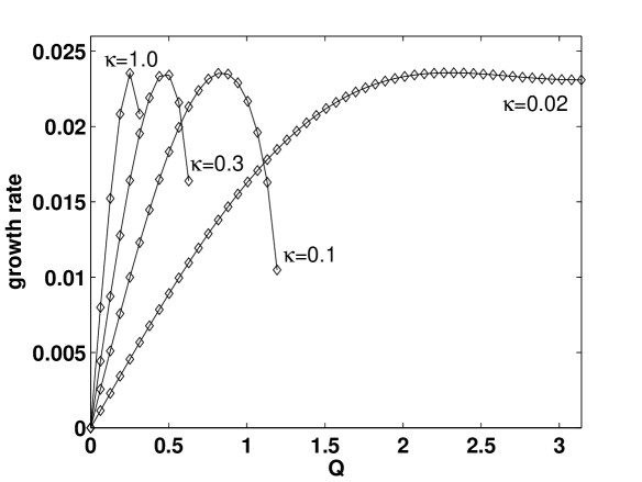
we depict the growth rate for different values of the coupling strength for a mode with $u_{0}=0.2$, $k=0$ and $N=100$. The inequality

$$\gamma\,u_{0}^{2}-2\kappa\,\sin^{2}\left(\frac{Q}{2}\right)\geq 0$$ (11)

puts a constraint on the allowed wave numbers. For relatively small coupling strength $\kappa=0.02$ the whole range of wave numbers $|Q|\leqslant\pi$ is responsible for the modulational instability, albeit with different weights. Enlarging $\kappa$ not only increasingly shifts the cut-off for the allowed wave numbers towards $Q=0$ but in addition makes the instability bands also narrower. In other words the modulational instability becomes more mode-selective. Nevertheless, the maximum of the growth rate

$$\Gamma_{max}=\frac{1}{2\omega_{0}}\gamma u_{0}^{2}\,,$$ (12)

is unaffected by alterations of $\kappa$, while its position

$$Q_{max}=2\sin^{-1}\left(\sqrt{\frac{\gamma u_{0}^{2}}{4\kappa}}\right)\,,$$ (13)

moves closer to zero with increasing coupling strength $\kappa$.

The way the growth rates with corresponding weights for perturbations at different wave numbers $Q$ contribute to a mean growth rate is determined by the quantity $\bar{\Gamma}$, reading:

$$\bar{\Gamma}=\frac{2}{N}\sum\limits_{n=0}^{N/2}\Gamma\left(Q=\frac{2\pi}{N}\,n,k=0\right)\,.$$ (14)

Figure 3: Mean growth rate versus the coupling strength. The parameter values used are the same as in Fig. 2.

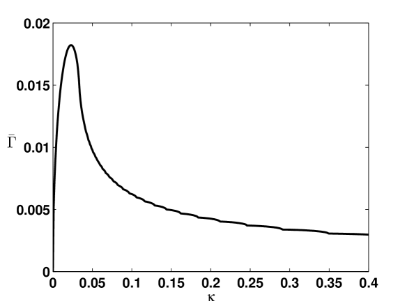
This quantifier is depicted in Fig. 3 as a function of the coupling strength $\kappa$. The maximum around $\kappa\simeq 0.023$ suggests that a sizable divergence of the perturbations is induced. To the left of its maximum the mean growth rate drops drastically while on its right the decrease considerably weakens.

IV Energy sharing and formation of arrays of breathers

In order to enhance the energy localization in the dynamics of Eq. (3) we propose the following scenario: An amount of energy $E_{0}=E_{total}/N$ is applied per unit which allows the activation of nonlinear, self-organized excitations of the chain.

Thus, the chain possesses a total energy $E_{total}=NE_{0}$. For an escape to take place we have: $E_{total}>E_{act}>\Delta E$. This inequality conveys the fact that more than just one unit governs the escape mechanism. The initial energy $E_{0}$ is supplied as follows: (i) First, the whole chain is elongated homogeneously along a fixed position $q_{0}$ near the bottom of the well. [Notice that from Eq. (8) it follows that this corresponds to a flat mode being equivalent to a $k=0$ plane-wave solution and thus $q_{0}=2u_{0}$.] (ii) Then, the position of all units and their momenta are iso-energetically randomized while keeping the total energy a constant—i.e. $E_{total}=NE_{0}=\mbox{const}$.

The random position values are chosen from a bounded interval $|q_{n}(0)-{q_{0}}|\leq\Delta q$ and, likewise, the random initial momenta, $|p_{n}(0)-p_{0}|\leq\Delta p$. From Eq. (5) for a plane-wave solution with wave number $k=0$ one deduces that $p_{0}=0$. The whole chain is thus initialized close to an almost homogeneous state, but yet sufficiently displaced ($\Delta q\neq 0$) in order to generate nonvanishing interactions, enabling the exchange of energy among the coupled units.

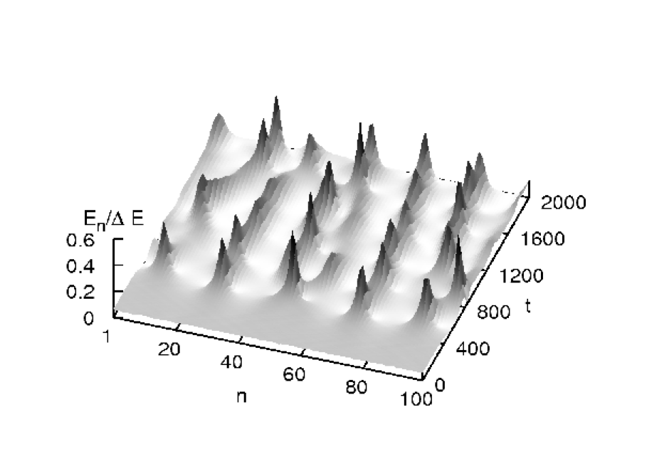
As the role of the deviation of the initial conditions from a completely homogeneous state for the instigation of the energy exchange process is concerned we observe that the attainment of an array of humps proceeds the faster the larger is the width $\Delta p$ and/or $\Delta q$. More precisely, due to the emergence of a modulational instability a pattern evolves in the course of time (of the order of $t\sim 5\times 10^{2}$) where for some lattice sites the amplitudes grow considerably whereas they remain relatively small in the adjacent regions. This feature is illustrated in Fig. 4, depicting the spatio-temporal evolution of the site-energy:

$$E_{n}=\frac{p_{n}^{2}}{2}\,+\,U(q_{n})\,+\,\frac{\kappa}{4}\left[\,\left(\,q_{n+1}-q_{n}\,\right)^{2}+\left(\,q_{n-1}-q_{n}\,\right)^{2}\,\right]\,.$$ (15)

The breather states possessing a relatively high energy occur spontaneously at an average distance of the inverse wave numbers $Q_{max}^{-1}$, corresponding to the maximal growth rate $\Gamma_{max}$ in (12). Upon moving, these breathers tend to collide inelastically with others. In fact, various breathers merge to form larger-amplitude breathers, proceeding preferably such that the larger-amplitude breathers grow at the expense of the smaller ones. As a result, a certain amount of the total energy becomes strongly concentrated within confined regions of the chain. This localization scenario is characteristic for nonlinear lattice systems Daumont , Bang -Tsironis .

For our simulations the set of coupled equations (3) has been numerically integrated by use of a fourth-order Runge-Kutta scheme. The accuracy of the calculation was checked by monitoring the conservation of the total energy with precision of at least $10^{-5}$. The investigated chain consists of $100$ coupled oscillators.

Figure 4: Spatio-temporal evolution of the energy distribution $E_{n}(t)$. Initially, the coordinates are uniformly distributed $(k=0)$ within the interval $|q_{n}(0)-{q_{0}}|\leq\Delta q$ with an average at ${q_{0}}=0.3$ and width $\Delta q=0.01$ and zero momenta—i.e., $p_{0}=\Delta p=0$. This yields a total energy $E_{total}=8.1\equiv 6.075\Delta E$. The parameter values are given by $a=1$, $\omega_{0}^{2}=2$, $N=100$, and $\kappa=0.3$.

To relate the energy localization with an escape over the barrier we note that in the beginning the average amount of energy contained in a single unit, $E_{0}={E_{total}}/{N}$, lies significantly below the barrier energy as expressed by the low ratio $E_{0}/\Delta E=0.06$. Thus, a single unit must acquire the energy content of at least $16$ nearby units before it is able to overcome the barrier.

Figure 5: Snapshots of the amplitudes $q_{n}(t)$ of a segment of the lattice covering ten oscillators, illustrating the formation of a localized structure with a subsequent barrier crossing event of the chain. Initial conditions are $q_{0}=0.45$, $\Delta q=0.01$, and $p_{0}=\Delta p=0$. Parameter values are $\omega_{0}^{2}=2$, $a=1$, $N=100$, and $\kappa=0.2$. Top panel: snapshot taken at time $t=473$: Emergence of localized structures. Bottom panel: snapshot taken at time $t=673$: Depicted is a segment of the lattice with one unit located beyond the barrier. The dashed lines in the ($q_{n}-n$)-plane designate the position of the potential’s minimum and maximum.

For further illustration we depict in Fig. 5 snapshots of $q_{n}(t)$ at two different instants of time. In the beginning the energy is virtually equally shared among all units (not shown). After a certain time has evolved, the local energy accumulation is enhanced in such a manner that at least one of the involved units possess enough energy to overcome the barrier. The question then is, does such an escaped unit continue its excursion beyond the barrier or can it even be pulled back into the bound chain formation ($q_{n}<q_{max}$) by the restoring binding forces exercised by its neighbors? On the other hand, the unit that has already escaped from the potential well might drag neighboring ones closer to or, in the extreme, even over the barrier. Thus, a concerted escape of the chain from the potential valley becomes plausible .

V Transition state

Whether a unit of growing amplitude can in fact escape from the potential well or is held back by the restoring forces of their neighbors depends on the corresponding amplitude ratio as well as on the coupling strength. The critical chain configuration—that is, the transition state separating bounded ($q_{n}<q_{max}$) from unbounded ($q_{n}>q_{max}$) lattice solutions—is determined by $\ddot{q}_{n}(t)=0$. The system of equations (3) then reduce to the stationary system of equations:

$$-\frac{\partial U}{\partial\tilde{q}_{n}}+\kappa[\tilde{q}_{n+1}+\tilde{q}_{n-1}-2\tilde{q}_{n}]=0\,.$$ (16)

Interpreting $n$ as a ’discrete’ time, with $1\leq n\leq N$, equation (16) describes the motion of a point particle in the inverted potential $-U(\tilde{q})$. This difference system can be cast in the form of a two-dimensional map by defining $x_{n}=\tilde{q}_{n}$ and $y_{n}=\tilde{q}_{n-1}$ Physicsreports , which gives

$$x_{n+1} = (\omega_{0}^{2}x_{n}-ax_{n}^{2})/\kappa+2x_{n}-y_{n}$$

$$y_{n+1} = x_{n}\,.$$ (17)

The fixed points of this map are found as

$$x_{0}=y_{0}=0\,,\qquad\qquad x_{1}=y_{1}=\frac{\omega_{0}^{2}}{a}\,.$$ (18)

A linear stability analysis reveals that $(x_{0},y_{0})$ represents an unstable hyperbolic equilibrium while at $(x_{1},y_{1})$ a stable center is located. The map is non-integrable. The stable and unstable manifolds of the hyperbolic point intersect each other, yielding homoclinic crossings as illustrated in Fig. 6.

Figure 6: First intersections of the stable $W_{s}$ (thin gray line) and the unstable $W_{u}$ manifold (thick dark line) of the hyperbolic point of the map in Eq. (17) at the map origin $(0,0)$. The parameter values are $\omega_{0}^{2}=2$, $a=1$, and $\kappa=1$. The homoclinic point labeled $(\tilde{q}_{n_{c}}^{h};\tilde{q}_{n_{c}+1}^{h})$ and its map iterate $(\tilde{q}_{n_{c}+1}^{h};\tilde{q}_{n_{c}+2}^{h})$ correspond on the consecutive lattice sites $n=n_{c},n_{c}+1,n_{c}+2$ to a decaying pattern whose amplitudes with $\tilde{q}_{n}^{h}>\tilde{q}_{n+1}^{h}$ are represented by the arrows of varying length in the schematic representation in the upper left corner. Map iterations of the homoclinic point $(\tilde{q}_{n_{c}+1}^{h};\tilde{q}_{n_{c}+2}^{h})$ result in further homoclinic points approaching asymptotically the hyperbolic point at the map origin.

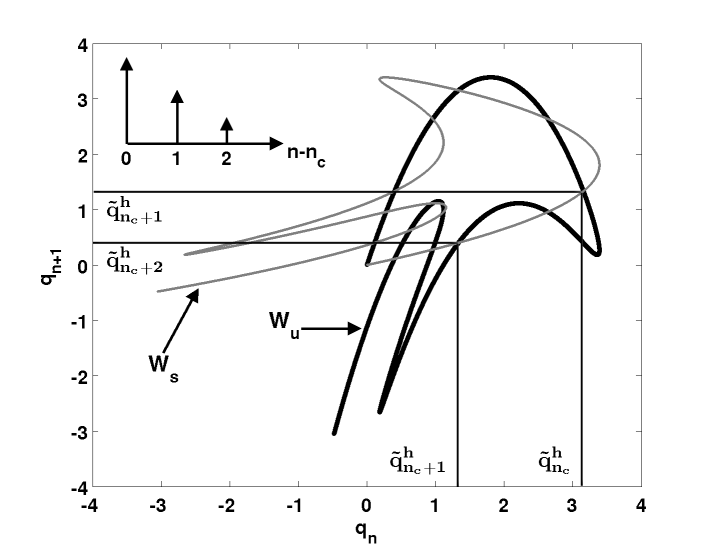
The corresponding homoclinic orbit of the map, consisting of the points of intersections between $W_{s}$ and $W_{u}$, is on the lattice chain equivalent to a stationary localized hump solution $\{\tilde{q}_{n}^{h}\}$, centered at site $n=n_{c}$, which resembles the form of a (pointed) hairpin (for details concerning the relation between homoclinic orbits and localized lattice solutions see Physicsreports and PRE96 ). In Fig. 7 profiles of this hairpin-like critical localized mode (c.l.m.), or critical nucleus, with displacements $\{\tilde{q}_{n}^{h}\}$ are depicted for several coupling strengths. We observe that the stronger the coupling is, the larger the maximal amplitude of the humps is, $\tilde{q}_{n_{c}}^{h}=\tilde{q}_{max}^{h}$, and the wider the spatial extension of the latter is. We underline that on a sufficiently extended lattice this c.l.m. represents a narrow chain formation with its width being much smaller than the total chain length.

Figure 7: Amplitude profile of the critical chain configuration, being symmetrically centered at site $n_{c}$, for different coupling strengths $\kappa=0.1$ (circles), $\kappa=0.3$ (diamonds), and $\kappa=1.0$ (triangles). For better illustration only we depict the central part of the lattice chain with sizable elongations. The parameter values are $\omega_{0}^{2}=2$ and $a=1$.

Equation (16) can be derived from an energy functional with vanishing kinetic energy, reading

$$E[\{\tilde{q}_{n}\}]=\sum_{n}\,\left(U(\tilde{q}_{n})+\frac{\kappa}{2}[\tilde{q}_{n}-\tilde{q}_{n-1}]^{2}\right)$$ (19)

with $\partial E/\partial\tilde{q}_{n}=0$. Apparently, with increasing coupling strength $\kappa$ a larger activation energy

$$E_{act}=E[\{\tilde{q}_{n}^{h}\}]$$ (20)

is required to bring the chain into its critical localized mode configuration.

The activation energies for different coupling strengths are depicted in Fig. 8.

Figure 8: Activation energy $E_{act}$ as a function of the coupling strength $\kappa$. Solid line: fitted data with slope $s=3.54\pm 0.01$. The remaining parameter values are $\omega_{0}^{2}=2$ and $a=1$.

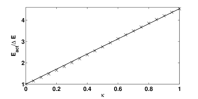
For small coupling the maximal amplitude $\tilde{q}_{max}^{h}$ is beyond but still close to $q_{max}=\omega_{0}^{2}/a$ [the position of the maximum of the potential $U(q)$] while the remaining units practically reside at the minimum of the potential $U(q)$. For larger couplings the maximal amplitude $\tilde{q}_{max}^{h}$ lies at larger distances beyond $q_{max}$. Most importantly, for escape we have that $\partial U(\tilde{q})/\partial\tilde{q}|_{\tilde{q}=\tilde{q}_{max}^{h}}<0$.

It can be shown that the critical localized mode, being associated with an unstable saddle point in configuration space, is indeed dynamically unstable. Setting $q_{n}(t)=\tilde{q}_{n}^{h}+w_{n}(t)$ with $|w_{n}|\ll 1$ the linearized equations of motion are derived as

$$\ddot{w}_{n}(t) = -\frac{\partial^{2}U({q}_{n})}{\partial q^{2}_{n}}\rvert_{q_{n}={\tilde{q}}_{n}^{h}}w_{n}(t)$$ (21)

$$+ \kappa[w_{n+1}(t)+w_{n-1}(t)-2w_{n}(t)]\,.$$

With the ansatz $w_{n}(t)=\phi_{n}\exp(\sqrt{\lambda}t)$ for the solution of (21) one arrives at an eigenvalue problem

$$\lambda\phi_{n}=-V_{n}\phi_{n}+\kappa[\phi_{n+1}+\phi_{n-1}-2\phi_{n}]\,,$$ (22)

with

$$V_{n}=\frac{\partial^{2}U({q}_{n})}{\partial q^{2}_{n}}\rvert_{q_{n}={\tilde{q}}_{n}^{h}}=\omega_{0}^{2}-2a\tilde{q}_{n}^{h}\,.$$ (23)

The second-order difference equation (22) is of the discrete stationary Schrödinger type, with a non-periodic potential $-V_{n}$, breaking the translational invariance so that localized solutions exist (so called stop-gap states). The evolution of the two-component vector $(\phi_{n+1},\phi_{n})^{T}$ is determined by the following Poincaré map:

$$\cal{M}: \begin{pmatrix}\phi_{n+1}\\ \phi_{n}\end{pmatrix}=\begin{bmatrix}E_{n}&-1\\ 1&0\end{bmatrix}\begin{pmatrix}\phi_{n}\\ \phi_{n-1}\end{pmatrix}\,,$$ (24)

with on-site energy $E_{n}=(\lambda+V_{n})/\kappa+2$. The nodeless even-parity ground state of Eq. (22), with its energy under the lower edge of the energy band of the passing band states, corresponds to an orbit of the linear map $\cal{M}$ being homoclinic to the hyperbolic equilibrium point at the origin $(0,0)$ of the map plane. For the presence of a hyperbolic equilibrium the following inequality has to be satisfied:

$$\operatorname{Trace}({\cal{M}})=E_{n}=\frac{\lambda+V_{n}}{\kappa}+2>2\,,$$ (25)

implying that $\lambda$ must fulfill the constraint

$$\lambda>\max_{n}(-V_{n})=2a\max_{n}\tilde{q}_{n}^{h}-\omega_{0}^{2}\,>0.$$ (26)

With the maximal amplitude of the c.l.m. lying beyond the barrier—viz., $\max_{n}\tilde{q}_{n}^{h}>\omega_{0}^{2}/a$—one finds

$$\lambda>\omega_{0}^{2}>0\,.$$ (27)

Therefore, the ground state belongs to a positive eigenvalue from which we deduce that perturbations of the corresponding solution in the time domain grow exponentially. Hence, if the kinetic energy overcomes the critical nucleus, the subsequent escape of its neighbors is initiated, which progress on the chain to the left and to the right of the hair pin as a propagating kink and anti-kink, respectively (see Refs. Sebastian ; LanBut ; MarHan1 ; MarHan2 ). In phase space the units move parallel to the unstable manifold of the hyperbolic equilibrium [which is related to the saddle point at the maximum of the potential $U(q)$], realizing in this way an efficient lowering of the total potential energy. Because the kinetic energy of this outward motion is consequently increasing, a return backwards over the barrier into the original well is hereby prevented. Fig. 9 illustrates the kink-antikink motion

Figure 9: The escape time $T_{esc}^{(n)}$ of the individual chain units versus position for collective escape and periodic boundary conditions for a chain consisting of $100$ units for one realization of initial conditions. The parameter values are $a=1$, $\omega_{0}^{2}=2$, $N=100$, and $\kappa=0.3$. The initial conditions are given by $q_{0}=0.45$, $\Delta q=0.1$, and $p_{0}=\Delta p=0$.

showing the escape time $T_{esc}^{(n)}$ of the units versus the position on the lattice. The escape time of a unit is defined as the moment at which it passes through the value $q_{esc}=5\,q_{max}$ beyond the barrier. We remark that $q_{esc}$ is chosen such that $U(q_{esc})$ is sufficiently lowered so that the return of an escaped unit over the barrier into the potential well is practically excluded. Consecutively, all oscillators manage to eventually climb over the barrier one after another in a relatively short time interval. (The position of the first escape event varies in general for random samples of initial conditions.)

VI Comparison with thermally activated escape

We next compare the microcanonical escape process with the corresponding thermally assisted escape process at a temperature $T$ RMP ; JSPHa ; Sebastian ; Lee ; Kraikivsky ; LanBut ; MarHan1 ; MarHan2 . The associated Langevin system reads

$$\frac{d^{2}q_{n}}{dt^{2}}\,+\,\frac{dU}{dq_{n}}-\kappa\,\left[\,q_{n+1}+q_{n-1}-2q_{n}\,\right]+\nu\frac{dq_{n}}{dt}+\xi_{n}(t)=0\,\,,$$ (28)

with a friction parameter $\nu$ and where $\xi_{n}(t)$ denotes a Gaussian distributed thermal, white noise of vanishing mean $<\xi_{n}(t)>=0$, obeying the well-known fluctuation-dissipation relation $<\xi_{n}(t)\xi_{n^{\prime}}(t^{\prime})>=2\nu k_{B}T\delta_{n,n^{\prime}}\delta(t-t^{\prime})$ with $k_{B}$ denoting the Boltzmann constant. We define the escape time of a chain as the mean value of the escape times of its units (see again above).

Escape times

Our results are summarized in Fig. 10

Figure 10: Mean escape time $T_{esc}$ vs. the ratio $E_{0}/\Delta E$ of energy per unit $E_{0}$ and the barrier energy $\Delta E$ for the noise-free case with initial $k=0$ mode (solid line) with $\Delta q=0.01$ and $p_{0}=\Delta p=0$ (for $q_{0}$, see text), the case with strongly randomized initial conditions (diamonds) where $-0.251\leq q_{n}(0)\leq 0.534$, $-0.251\leq p_{n}(0)\leq 0.534$, and the noise-assisted escape (dashed line), respectively. The parameter values are $\omega_{0}^{2}=2$, $a=1$, $\kappa=0.3$, and the friction strength is $\nu=0.1$. The inset depicts the same data, but now plotted versus the effective Arrhenius factor $\Delta E/E_{0}$.

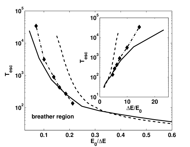
depicting the mean escape time as a function of $E_{0}/\Delta E$. The averages were performed over $500$ realizations of random initial conditions or the noise in the microcanonical and Langevin systems, respectively. For the deterministic and conservative system (3) the excitation energy $E_{0}$ is given by the (average) initial energy content of one unit $E_{0}=E_{total}/N$. For the simulations we varied $q_{0}$ while keeping $\Delta q=0.01$ and $p_{0}=\Delta p=0$ and obtained thus different values of $E_{total}$. In the case of the Langevin system (28) for sufficiently low $T$ the energy $E_{0}$ is taken as the thermal energy $k_{B}T$. This ratio thus corresponds to the inverse Arrhenius factor RMP ; indeed, at sufficient low temperature (large ratio $\Delta E/E_{0}$) the logarithmic escape time follows an almost linear behavior versus the Arrhenius factor, as expected for a noise-driven escape at weak noise strength RMP .

The Langevin equations were numerically integrated using a two-order Heun stochastic solver scheme Langevin_Numerics . In both cases there occurs a rather distinct decay of $T_{esc}$ with growing ratio $E_{0}/\Delta E$ in the low energy region. This effect weakens gradually upon further increasing $E_{0}$. Remarkably, for low $E_{0}$ (indicated as the breather region in the plot) the escape proceeds distinctly faster for the noise-free case as compared with a situation of a chain that is coupled to a heat bath at temperature $T$. This implies a large enhancement of the rate of escape as compared to the thermal rate. Near $E_{0}/\Delta E\geq 0.36$, there occurs a crossover, with the mean escape time of the deterministic system at even higher ratios closely following that of the thermal Langevin dynamics. At these values the escape times become comparable with the relaxation time which is determined by the inverse of the friction strength. Apparently in the region of lower $k_{B}T$ nonlinear excitations are damped out in the Langevin system at longer time scales. Hence they will not accelerate the escapes in the case with fluctuations and damping.

To sharpen our finding that the escape proceeds typically faster in the noiseless situation as compared to the case with a coupling to a heat bath, we investigated also the escape process of non-flat chain patterns starting out from strongly randomized initial conditions. For these initial conditions the coordinates and momenta are chosen at random from fairly broad ranges $-0.251\leq q_{n}(0)\leq 0.534$ and $-0.251\leq p_{n}(0)\leq 0.534$. For various energy values the averages were performed over $100$ realizations of initial conditions belonging to iso-energetic configurations with ratio $E_{0}/\Delta E$ each.

The findings for the mean escape time as a function of the mean initial energy content of the units relative to the barrier height $E_{0}/\Delta E$ are included in Fig. 10 with the diamond symbols. Most importantly, even for random initial conditions the mean escape time assumes smaller values in the microcanonical situation as compared to the Langevin dynamics. This underpins our general statement that noiseless escape indeed proceeds faster than thermally activated escape.

We note that the breathers present robust chain configurations that are formed rather fast as compared to the escape time. In contrast, the forever impinging stochastic forces seemingly impede a fast growth of the critical nucleus and may even cause a possible destruction of the critical chain formation, leading to re-crossings of the transition region, which only hampers a speedy escape. This inhibition for escape is most effective at small ratios of $E_{0}/\Delta E$, being induced either by high barrier heights, or low temperatures (implying a small $E_{0}$). A deterministic scenario thus presents a more favorable route towards accelerated escape in situations with very weak noise or very large barrier heights. Having performed also simulations for more general situations (i) with nonharmonic, nonlinear chain interactions, (ii) in higher dimensions, and (iii) with differing on-site potentials, we find preparation that the phenomenon of an enhanced, noise-free escape remains robust in regimes of a large effective Arrhenius factor with the latter given by the ratio of the barrier height $\Delta E$ and the initial energy per unit, $E_{0}$.

VII Optimal coupling and resonance structure in the escape process

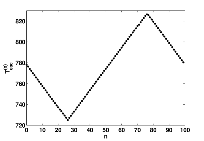
Furthermore, we study the impact of the coupling strength $\kappa$ on the escape process. The results concerning the mean escape time are illustrated with Fig. 11.

Figure 11: Resonant behavior in the mean escape time $T_{esc}$ as a function of the coupling strength $\kappa$ with the remaining parameter values as in Fig. 4. The initial conditions are for the coordinates $q_{0}=0.45$ and $\Delta q=0.1$ and for the momenta $p_{0}=\Delta p=0$. The averages were performed over $500$ realizations of random initial conditions.

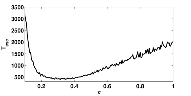
Strikingly, the mean escape time exhibits a resonance structure; viz., there exists a coupling strength ($\kappa_{res}=0.31$) for which the escape proceeds faster than for all other couplings strengths. Upon lowering $\kappa<\kappa_{res}$ we notice a substantial rise of the escape time while for $\kappa>\kappa_{res}$ the graph exhibits only a moderately growing slope with growing coupling strength $\kappa$. In this sense $\kappa_{res}=0.31$ from Fig. 11  represents indeed the optimal coupling strength for which escape is achieved within a minimal amount of time. Finally, outside the range $\kappa\in[0.05\,,\,1.5]$ not even the escape of a single unit has been observed. The reason is that the time scale for a pronounced formation of energy concentration, being vital for escape (due to breather coalescence and energy accumulation in the critical localized mode), exceeds the simulation time (taken here as $t=5000$).

A physical explanation for the appearance of a resonance-like structure can be given in terms of the different degrees of instability of the underlying motion facilitating the destruction of the initial flat mode by modulational perturbations. We recollect that with the variation of the perturbation strength the growth rate changes (cf. Sec. III) from a more flat to a strongly curved single-peaked structure. To illustrate the impact of the growth rate on the degree of localization of emerging patterns we present in Fig. 12

Figure 12: Spatially localized structure at $t=500$ for three different coupling strengths. Initial conditions and parameter values as in Fig. 4 except for the coupling strengths (a) $\kappa=0.05$, (b) $\kappa=0.31$, and (c) $\kappa=1.00$.

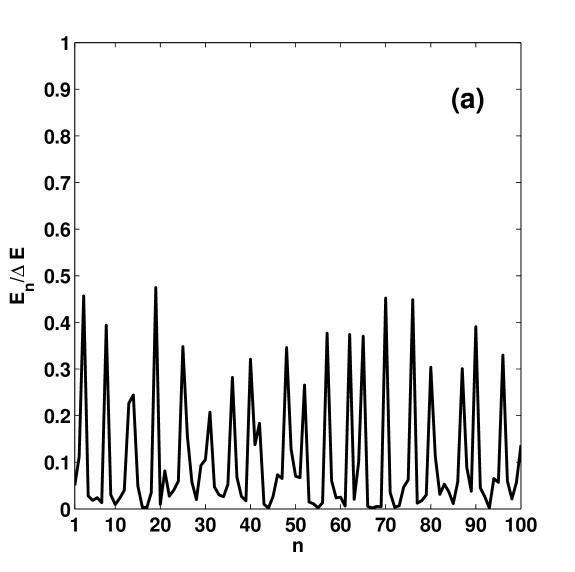
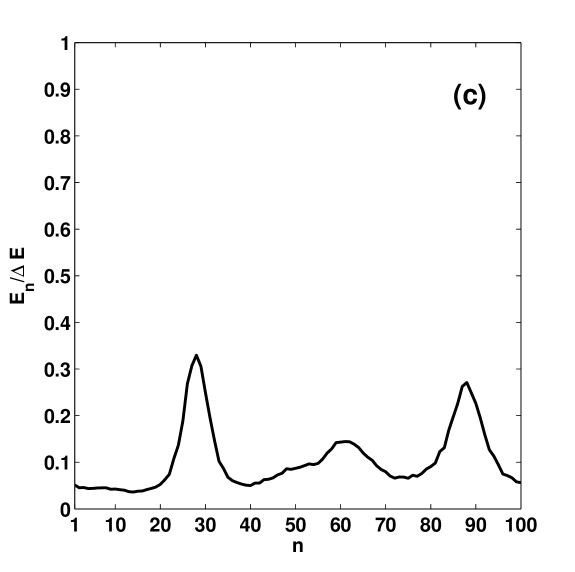
the energy distribution defined in Eq. (15) at an early instant of time—namely, after the formation of the spatially localized structure due to spontaneous modulational instability has taken place. For comparison, patterns for three coupling strengths are shown. In all cases a number of isolated localized humps are formed. The number of humps, $N_{humps}$, can be attributed to the wave number at maximal growth rate as follows: $\lambda_{pattern}N_{humps}=N$ and $\lambda_{pattern}=2\pi/Q_{max}$. Most importantly, the number of humps (besides their height and width) regulates how the total energy is shared among them. Clearly, for $\kappa=0.31$ [Fig. 12 (b)] the energy is more strongly localized (fewer humps and of higher height) than in the case of $\kappa=0.09$ [Fig. 12 (a)]. In comparison for $\kappa=1$ [Fig. 12 (c)] the number of humps is further diminished, but they are of lower height than most of the humps for $\kappa=0.31$. In fact, for $\kappa=0.31$ the energy contained in the unit at site $n=35$ is close to the one of the barrier. Thus, a localized pattern appropriate for escape is provided already by the mechanism of modulational instability. In particular, no further (major) energy accumulation, which would delay the escape process considerably, is hence required.

To gain further insight into the efficiency of energy localization it is illustrative to suppose that the whole lattice can be divided into a periodic array of (non-interacting) segments where each of them supports a single localized hump. The energy of one segment is determined by

$$E_{s}=\frac{E_{total}}{N_{humps}}=\frac{E_{total}}{N/\lambda_{pattern}}\,.$$ (29)

Defining $e_{s}=E_{s}/\Delta E$ as the ratio of the energy per segment to the net barrier energy we obtain

$$e_{s}=\frac{2\pi E_{total}}{Q_{max}N\Delta E}\,.$$ (30)

Appropriate conditions for escape are provided when the energy contained in each segment, $e_{s}$, is close to the activation energy, $e_{act}$, measured in units of the barrier energy—i.e., $e_{act}=E_{act}/\Delta E$. The efficiency of energy localization is then determined by the following ratio

$$\chi=\frac{e_{s}}{e_{act}}\,.$$ (31)

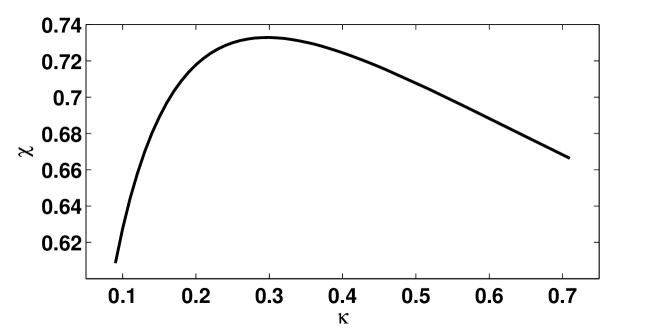
For a given value of the coupling strength $\kappa$ the activation energy is known; cf. Fig. 8. Fixing the initial energy and using Eq. (10) we infer the value of $Q_{max}$ and finally using Eqs. (30) and (31) we obtain $\chi$. In Fig. 13 the ratio $\chi$ is plotted as a function of the coupling strength $\kappa$. The plot exhibits a maximum at $\kappa=0.3$, which corroborates the finding of the resonance found for the escape versus coupling strength as depicted in Fig. 11. Moreover, the curvature of the graphs of Figs. 11 and 13 are similar.

Figure 13: The ratio $\chi$ defined in Eq. (31) as a function of the coupling strength $\kappa$. The parameter values are $\omega_{0}^{2}=2$ and $a=1$. The initial conditions are given by $q_{0}=0.45$ and $p_{0}=0$.

VIII Influence of chain length on the escape time

We also study the influence of ”size”—i.e., the number of oscillators, $N$, on the escape process. A general constraint on the escape process arising from varying the chain length is formulated. We discuss the escape time statistics for chains with constant energy density and for chains with fixed total energy, but varying number of oscillators, respectively. Our studies apply to a homogeneous initial state ($k=0$ mode).

First of all, the initial homogeneous state must become unstable with respect to a modulational instability. With relation (11) a constraint is established on the allowed wave numbers, giving rise to the modulational instability. They form a discrete set, and we can derive a lower bound for the number of oscillators, $N_{min}$, needed for the onset of the modulational instability:

$$N_{min}>\frac{\pi}{\arcsin\left(\sqrt{\frac{\gamma u_{0}^{2}}{2{\kappa}}}\right)}.$$ (32)

In the case of $u_{0}^{2}>2{\kappa}/\gamma$ the initial homogeneous state is always unstable, independent of the number of oscillators, $N$. However, for an initial state in the weakly nonlinear regime, which means $u_{0}^{2}<2{\kappa}/\gamma$, the inequality (32) yields a condition for the minimal number of units on the chain that are necessary for modulational instability. On the other hand, once the conditions are provided that the chain be able to adopt the transition state, the addition of further lattice sites beyond a certain number leaves the activation energy unaltered. This is due to the fact that the transition state is represented by the c.l.m. which is strongly localized in space with exponential decaying tails.

Case with constant energy density

Let us first consider chains with constant energy density $\rho=E_{total}/N=const$. One would at first glance expect a faster escape with increasing number of oscillators and thus with increasing total energy. This is, however, not necessarily the case. For an explanation it is suitable to consider the limit of very long chains, $N\rightarrow 1000$.

Figure 14: First, mean, and last escape time $T_{esc}$ as a function of the chain length, $N$. The parameter values are $\omega_{0}^{2}=2$, $a=1$, and $\kappa=0.2$. The initial conditions are given by $q_{0}=0.50$, $\Delta q=0.01$, and $p_{0}=\Delta p=0$.

In Fig. 14 the average time for which the first and last escape incidents of a unit take place is depicted versus varying chain length $N$. The averages were performed again over $500$ realizations of random initial conditions. In addition, we as well depict the mean escape time of the chain. We set the initial coordinates around a mean value of $q_{0}=0.50$ and spread at $\Delta q=0.01$, yielding $\rho=0.156\Delta E$. Apparently the longer the chain is, the more humps (breathers) that are formed due to the modulational instability. This offers the possibility that a larger number of interacting breathers contribute to an enhanced energy localization in a confined region of the chain which in turn boosts the formation of the critical localized mode. Hence, the time it takes for the first unit to escape shrinks with increasing chain length, while the last escape time increases due to the enlarged number of escaping units. Also, the mean escape time becomes insensitive to variations of the chain length for sufficiently large length $N\geq 500$, and thus it tends to saturate.

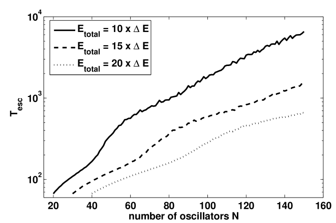
Fixed total energy

We next consider the situation when a fixed amount of total energy—i.e., $E_{total}=const$—is provided to the system and the number of units on the lattice is varied. To obtain a certain value of $E_{total}$ upon altering the number of units, $N$, we adopted $q_{0}$ appropriately while keeping $\Delta q=0.01$ and $p_{0}=\Delta p=0$ fixed. The maximal energy content per unit is restricted to the range $E_{0}<0.5\Delta E$. The results for the mean escape time are depicted in Fig. 15. Generally, we observe an increase of $T_{esc}$ with growing $N$. Interestingly enough, the slope passes through intermediate stages of sub-exponential, hyper-exponential and eventually approaches an exponential behavior.

Figure 15: Mean escape time $T_{ecs}$ as a function of the number of oscillators, $N$, for different values of $E_{total}$. For the choice of $q_{0}$, see text. Furthermore $\Delta q=0.01$ and $p_{0}=\Delta p=0$. The parameter values are $\omega_{0}^{2}=2$, $a=1$, $\kappa=0.2$, and $E_{total}$ as depicted in the legend.

IX Summary

In this paper we have explored the conservative and deterministic dynamics of a one-dimensional chain consisting of linearly coupled anharmonic oscillators that are placed into a cubic on-site potential. Attention has been paid to the collective barrier crossing of the whole chain. Initially the system is placed into a metastable state for which all units are trapped near the bottom of the potential. An overcoming of the barrier of the whole chain is prevented at short initial times because of a too high net barrier height. Nevertheless, as we convincingly demonstrated, the spontaneous formation of localized modes upon evolving time serves to enrich energetically a segment on the chain to such a degree that it adopts the transition state energy in assuming the form of a hairpin. We have shown that the associated critical localized lattice state is dynamically unstable and eventually a barrier crossing proceeds as the propagation of a kink-antikink-like pair along the chain. Strikingly, there exists a resonant-like coupling strength $\kappa$ for which the escape time (rate) becomes minimal (maximal), cf. Fig. 11.

In view of potential applications we note that this deterministic collective escape process provides nonlinear systems with the unique possibility to self-promote their activation dynamics. Particularly, the ability to operate efficiently—i.e., exhibiting an enhanced collective coherent escape—although not optimally initialized (meaning that one starts out with a far too low energy density compared to the barrier height) underpins the beneficial use of this physical scenario. Remarkably, while at weak thermal noise the rate of thermal escape is exponentially suppressed, a deterministic nonlinear breather dynamics yields a robust critical nucleus configuration, which in turn causes an enhancement of the noise-free escape rate. Thus, the freezing out of noise may prove advantageous for transport in metastable landscapes, whenever the deterministic escape dynamics can be launched in a single shot via an initial energy supply.

Acknowledgments

This research has been supported by SFB-555 (L.S.-G. and S.F.) and, as well, by the joint Volkswagen Foundation Projects No. I/80424 (P.H.) and No. I/80425 (L.S.-G.).

References

- (1) P. Hänggi, P. Talkner and M. Borkovec, Rev. Mod. Phys. 62, 251 (1990).
- (2) P. Hänggi, J. Stat. Phys. 42, 105 (1986); J. Stat. Phys. 44, 1003 (1986).
- (3) J. S. Langer, Ann. Phys. (N.Y.) 54, 258 (1969).
- (4) W. Sung and P. J. Park, Phys. Rev. Lett.77, 783 (1996).
- (5) P. J. Park and W. Sung, Phys. Rev. E 57, 730 (1998); J. Chem. Phys. 108, 3013 (1998); ibid 111, 5259 (1999).
- (6) I. E. Dikshtein, N. I. Polzikova, D. V. Kuznetsov, and L. Schimansky-Geier, J. Appl. Phys. 90, 5425 (2001); I. E. Dikshtein, D. V. Kuznetsov and L. Schimansky-Geier, Phys. Rev. E 65, 061101 (2002).
- (7) K. L. Sebastian and A. K. R. Paul, Phys. Rev. E 62, 927 (2000).
- (8) S. Lee and W. Sung, Phys. Rev. E 63, 021115 (2001) ; K. Lee and W. Sung, Phys. Rev. E 64, 041801 (2001).
- (9) P. Kraikivsky, R. Lipowsky and J. Kiefeld, Europhys. Lett. 66, 763 (2004).
- (10) M. T. Dowtown, M. J. Zuckermann, E. M. Craig, M. Plischke and H. Linke, Phys. Rev. E 73, 011909 (2006).
- (11) P. Hänggi, F. Marchesoni and F. Nori, Ann. Physik (Leizig) 14, 51 (2005); R. D. Astumian and P. Hänggi, Physics Today 55 (11), 33 (2002); P. Reimann and P. Hänggi, Appl. Phys. A 75, 169 (2002).
- (12) D. Hennig, L. Schimansky-Geier and P. Hänggi, Europhys. Lett. 78, 20002 (2007).
- (13) M. I. Rabinovich, P. Varona, A. I. Selverston and H. D. I. Abarbanel, Rev. Mod. Phys. 78, 1213 (2006).
- (14) M. Sato, B. E. Hubbard and A. J. Sievers, Rev. Mod. Phys. 78, 137 (2006).
- (15) S. Flach and C. R. Willis, Phys. Rep. 295, 181 (1998).
- (16) S. Takeno and G. P. Tsironis, Phys. Lett. A 343, 274 (2005).
- (17) N. Lazarides, M. Eleftheriou and G. P. Tsironis, Phys. Rev. Lett. 97, 157406 (2006); M. V. Ivanchenko, O. I. Kanakov, K. G. Mishagin and S. Flach, Phys. Rev. Lett. 97, 025505 (2006); S. Flach, M. V. Ivanchenko and O. I. Kanakov, Phys. Rev. E 73, 036618 (2006); J. Cuevas, P. G. Kevrekidis, D. J. Frantzeskakis and A. R. Bishop, Phys. Rev. B 74, 064304 (2006); S. Flach and A. Gorbach, Int. J. Bifurcation and Chaos 16, 1645 (2006); P. Maniadis and S. Flach, Europhys. Lett. 74, 452 (2006); S. Aubry, Physica D 216, 1 (2006).
- (18) M. Remoissenet, Waves called Solitons (Springer-Verlag, Berlin, 1978).
- (19) R. S. MacKay and S. Aubry, Nonlinearity 7, 1623 (1994).
- (20) S. Aubry, Physica D 103, 201 (1997). (1998).
- (21) P. Marqui, J. M. Bilbault and M. Remoissenet, Phys. Rev. E 51, 6127 (1995).
- (22) H. S. Eisenberg, Y. Silberberg, R. Morandotti, A. R. Boyd and J. S. Aitchison, Phys. Rev. Lett. 81, 3383 (1998).
- (23) P. Binder, D. Abraimov, A. V. Ustinov, S. Flach and Y. Zolotaryuk, Phys. Rev. Lett. 84, 745 (2000).
- (24) Yu. S. Kivshar and M. Peyrard M., Phys. Rev. A 46, 3198 (1992); T. Dauxois, S. Ruffo and A. Torcini, Phys. Rev. E 56, R6229 (1997); T. Cretegny, T. Dauxois, S. Ruffo, and A. Torcini, Physica D 121, 109 (1998).
- (25) K. W. Sandusky and J. B. Page, Phys. Rev. B 50, 866 (1994).
- (26) T. Dauxois and M. Peyard, Phys. Rev. Lett. 70, 3935 (1993).
- (27) M. Peyrard, Physica D 119, 184 (1998).
- (28) Yu. S. Kivshar, Phys. Rev. E 48, 4132 (1993).
- (29) I. Daumont, T. Dauxois and M. Peyrard, Nonlinearity 10, 617 (1997).
- (30) O. Bang and M. Peyrard, Phys. Rev. E 53, 4143 (1996).
- (31) J. L. Marn and S. Aubry, Nonlinearity 9, 1501 (1996).
- (32) T. Dauxois, S. Ruffo, and A. Torcini, Phys. Rev. E 56, R6229 (1997).
- (33) T. Cretegny, T. Dauxois, S. Ruffo and A. Torcini, Physica D 121, 109 (1998).
- (34) Yu. A. Kosevich and S. Lepri, Phys. Rev. B 61, 299 (2000).
- (35) K. Ullmann, A. J. Lichtenberg and G. Corso, Phys. Rev. E 61, 2471 (2000).
- (36) V. V. Mirnov, A. J. Lichtenberg and H. Guclu, Physica D 157, 251 (2001).
- (37) M. Eleftheriou and G. P. Tsironis, Physica Scripta 71, 318 (2005).
- (38) D. Hennig and G. P. Tsironis, Phys. Rep. 307, 333 (1999).
- (39) D. Hennig, K.Ø. Rasmussen, H. Gabriel, and A. Bülow, Phys. Rev. E 54, 5788 (1996).
- (40) P. V. Petukhov P. V. and V. L. Pokrovskii, Sov. Phys. JETP 36, 336 (1973) [Zh. Eksp. Teor.Fiz. 63, 634 (1972).
- (41) S. Fugmann, D. Hennig, L. Schimansky-Geier and P. Hänggi, in preparation.
- (42) P. Hänggi, F. Marchesoni and P. Sodano, Phys. Rev. Lett. 60, 2563 (1998).
- (43) P. Hänggi and F. Marchesoni, Phys. Rev. Lett 77, 787 (1996).
- (44) Card T.C., Introduction to Stochastic Differential Equations, Chapt. 7, Monographs in Pure and Appl. Mathematics, Vol. 114, (M. Dekker, Inc., New York, 1988).