A Magnetohydrodynamic Boost for Relativistic Jets

Abstract

We performed relativistic magnetohydrodynamic simulations of the hydrodynamic boosting mechanism for relativistic jets explored by Aloy & Rezzolla (2006) using the RAISHIN code. Simulation results show that the presence of a magnetic field changes the properties of the shock interface between the tenuous, overpressured jet ($V^{z}_{j}$) flowing tangentially to a dense external medium. Magnetic fields can lead to more efficient acceleration of the jet, in comparison to the pure-hydrodynamic case. A “poloidal” magnetic field ($B^{z}$), tangent to the interface and parallel to the jet flow, produces both a stronger outward moving shock and a stronger inward moving rarefaction wave. This leads to a large velocity component normal to the interface in addition to acceleration tangent to the interface, and the jet is thus accelerated to larger Lorentz factors than those obtained in the pure-hydrodynamic case. Likewise, a strong “toroidal” magnetic field ($B^{y}$), tangent to the interface but perpendicular to the jet flow, also leads to stronger acceleration tangent to the shock interface relative to the pure-hydrodynamic case. Overall, the acceleration efficiency in the “poloidal” case is less than that of the “toroidal” case but both geometries still result in higher Lorentz factors than the pure-hydrodynamic case. Thus, the presence and relative orientation of a magnetic field in relativistic jets can significant modify the hydrodynamic boost mechanism studied by Aloy & Rezzolla (2006).

1 Introduction

Relativistic jets have been observed in active galactic nuclei (AGN) and quasars (e.g., Urry & Pavovani 1995; Ferrari 1998), in black hole binaries (microquasars) (e.g., Mirabel & Rodiriguez 1999), and are also thought to be responsible for the jetted emission from gamma-ray bursts (GRBs)(e.g., Zhang & Mészáros 2004; Piran 2005; Mészáros 2006). Proper motions observed in jets from microquasars and AGNs imply jet speeds from $\sim 0.9c$ up to $\sim 0.999c$, and Lorentz factors in excess of $\Gamma\sim$ 100 have been inferred for GRBs. The acceleration mechanism(s) capable of boosting jets to such highly-relativistic speeds has not yet been fully established.

The most promising mechanisms for producing relativistic jets involve magnetohydrodynamic centrifugal acceleration and/or magnetic pressure driven acceleration from the accretion disk around compact objects (e.g., Blandford & Payne 1982; Fukue 1990), or direct extraction of rotational energy from a rotating black hole (e.g., Penrose 1969; Blandford & Znajek 1977). Recent General Relativistic Magneto-Hydrodynamic (GRMHD) simulations of jet formation in the vicinity of strong gravitational field sources, such as black holes or neutron stars, show that jets can be produced and accelerated by the presence of magnetic fields which are significantly amplified by the rotation of the accretion disk and/or the frame-dragging of a rotating black hole (e.g., Koide et al. 1999, 2000; Nishikawa et al. 2005; Mizuno et al. 2006b; De Villiers et al. 2005; Hawley & Krolik 2006; McKinney & Gammie 2004; McKinney 2006). The presence of strong magnetic fields is likely in areas close to the formation and acceleration region of relativistic jets. In the context of GRBs, standard scenarios invoke a fireball that is accelerated by thermal pressure during the initial free expansion phase (e.g., Mészáros et al. 1993; Piran et al. 1993). Magnetic dissipation may occur during the expansion, and a fraction of the dissipated energy may be used to further accelerate the fireball (e.g., Drenkhahn & Spruit 2002). Whether one considers the fate of the collapsing core of a very massive star (Woosley 1993), or the merger of a neutron star binary system (Paczynski 1986), the differentially rotating disks that feed the newly born black hole are likely to amplify any present seed field through magnetic braking and the magnetorotational instability (MRI) proposed by Balbus $\&$ Hawley (1991, 1998). Numerical solutions of the coupled Einstein-Maxwell-MHD equations (e.g., Stephens et al. 2006, and references therein) confirm the expected growth of seed fields, even to the point at which the fields become strong enough to be dynamically important.

Recently, Aloy & Rezzolla (2006) investigated a potentially powerful acceleration mechanism in the context of purely hydrodynamical flows, posing a simple Riemann problem. If the jet is hotter and at much higher pressure than a denser colder external medium, and moves with a large velocity tangent to the interface, the relative motion of the two fluids produces a hydrodynamical structure in the direction perpendicular to the flow (normal to the interface), composed of a “forward shock” moving away from the jet axis, and a “reverse shock” (or a rarefaction wave) moving toward the jet axis. Aloy & Rezzolla (2006) label this pattern either ${}_{\leftarrow}SCS_{\rightarrow}$, or ${}_{\leftarrow}RCS_{\rightarrow}$), where ${}_{\leftarrow}S$ refers to the reverse shock, (${}_{\leftarrow}R$ to the reverse rarefaction wave), $S_{\rightarrow}$ to the forward shock, and $C$ to the contact discontinuity between the two fluids. In the case ${}_{\leftarrow}RCS_{\rightarrow}$, the rarefaction wave propagates into the jet and the low pressure wave leads to strong acceleration of the jet fluid into the ultrarelativistic regime in a narrow region near the contact discontinuity. This hydrodynamical boosting mechanism is very simple and powerful, but is likely to be modified by the effects of magnetic fields present in the initial flow, or generated within the shocked outflow.

Here, we investigate the effect of magnetic fields on the boost mechanism proposed by Aloy & Rezzolla (2006). We find that the presence of magnetic fields in the jet can provide even more efficient acceleration of the jet than possible in the pure-hydrodynamic case. The highly significant role magnetic fields may play in accretion flows (e.g., Miller et al. 2006) and in core-collapse supernovae (e.g., Woosley $\&$ Janka 2005) is perhaps echoed in the collimated relativistic outflows from some compact stellar remnants.

2 Numerical Method

In order to study the magnetohydrodynamic boost mechanism for relativistic jets, we use a 1-dimensional special relativistic MHD (RMHD) version of the 3-dimensional GRMHD code “RAISHIN” in Cartesian coordinates (Mizuno et al. 2006a). A detailed description of the code and its verification can be found in Mizuno et al. (2006a). In the simulations presented here we use the piecewise parabolic method for reconstruction, the Harten, Lax, & van Leer (HLL) approximate Riemann solver (Harten et al. 1983), a flux constrained transport scheme to keep the magnetiic fields divergence free (Tot́h 2000), and Noble’s 2D primitive variable inversion method (Noble et al. 2006).

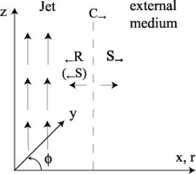
Figure 1: Schematic picture of our simulations.

We consider the Riemann problem consisting of two uniform initial states (a left- and a right state) with different and discontinuous hydrodynamic properties specified by the rest-mass density $\rho$, the gas pressure $p$, the specific internal energy $u$, the specific enthalpy $h\equiv 1+u/c^{2}+p/\rho c^{2}$, and with velocity component $v^{t}=v^{z}$ (the jet-direction) tangent to the initial discontinuity. We consider the right state (the medium external to the jet) to be a “colder” fluid with a large rest-mass density and essentially at rest. Specifically, we select the following initial conditions: $\rho_{R}=10^{-2}\rho_{0}$, $p_{R}=1.0\rho_{0}c^{2}$, $v^{n}_{R}=v^{x}_{R}=0.0$, and $v^{t}_{R}=v^{z}_{R}=0.0$, where $\rho_{0}$ is an arbitrary normalization constant (our simulations are scale-fee) and $c$ is the speed of light in vacuum, $c=1$. The left state (jet region) is assumed to have lower density, higher temperature and higher pressure than the colder, denser right state, and to have a relativistic velocity tangent to the discontinuity surface. Specifically, $\rho_{L}=10^{-4}\rho_{0}$, $p_{L}=10.0\rho_{0}c^{2}$, $v^{n}_{L}=v^{n}_{L}=0.0$, and $v^{t}_{L}=v^{z}_{L}=0.99c$ ($\gamma_{L}\simeq 7$) (in Table 1 these conditions are collectively labeled as case HDA). The fluid satisfies an adiabatic $\Gamma-law$ equation of state with $\Gamma=4/3$. The relevant sound speeds are $a_{j}=0.57735c$ in the jet flow, and $a_{e}=0.57663c$ in the external medium, where the sound speed is given by $a=\sqrt{\Gamma p/\rho h}$. We note that if the adiabatic index were $\Gamma=5/3$, the sound speeds would be $a_{j,e}\sim 0.82c$. These velocities exceed the maximum physically allowed sound speed $a=c/\sqrt{3}$. Therefore we choose the adiabatic index to be $\Gamma=4/3$ in our simulations. Figure 1 shows a schematic depiction of the geometry of our simulations.

To investigate the effect of magnetic fields, we consider the following left state field geometries: “poloidal”, $B^{z}=6.0\sqrt{\rho_{0}c^{2}}$ ($B^{{}^{\prime}}_{z}=6.0\sqrt{\rho_{0}c^{2}}$), in the MHDA case, and “toroidal” (not truly toroidal but we use this designation for simplicity), $B^{y}=42.0\sqrt{\rho_{0}c^{2}}$ ($B^{{}^{\prime}}_{y}=6.0\sqrt{\rho_{0}c^{2}}$), in the MHDB case (see Table1), where $B^{{}^{\prime}}_{i}$ is the magnetic field measured in the jet fluid frame ($B^{{}^{\prime}}_{y}=B^{y}/\gamma$, $B^{{}^{\prime}}_{z}=B^{z}$). Although the strength of the magnetic field measured in the laboratory frame ($B^{i}$) in the left state is larger in the MHDB case than the MHDA case, the magnetic pressure ($p_{mag}$) is the same as that of the MHDA case ($p_{mag}=(B^{{}^{\prime}})^{2}/2$). The relevant Alfvén speed in the left state is $v_{Aj}=0.68825c$, whereas the Alfvén speed $v_{A}$ is given by $v_{A}=\sqrt{[(B^{{}^{\prime}})^{2}/c^{2}]/[\rho h+(B^{{}^{\prime}})^{2}/c^{2}]}$.

For comparison, the HDB case listed in Table 1 is a high gas pressure, pure-hydrodynamic case ($p_{L}=28.0\rho_{0}c^{2}$). In this case the gas pressure $p_{L}$ in left state is equal to the total pressure ($p_{tot}$) in the MHD cases ($p_{tot}=p_{gas}+p_{mag}$) in the left state.

We employ free boundary conditions in all-directions. The simulations are performed in the region $-0.2\leq x\leq 0.2$ with 6400 computational zones ($\Delta x=6.25\times 10^{-5}$) until simulation time $t=0.1$. We emphasize that our simulations are scale-fee. If we specify a system of size $L=10^{7}$ cm ($\Delta L\simeq 6.25\times 10^{2}$ cm), a simulation time of $t=0.2$ corresponds to about $0.06$ msec. The units of magnetic field strength and pressure depend on the normalization of the density. If we take, for example, the density unit to be $\rho_{0}=10^{-20}\,\rm{g\,cm}^{-3}$, the magnetic field strength unit is about $3$ G and the pressure unit is $P\simeq 10\,\rm{dyn\,cm}^{-2}$.

3 Results

3.1 Effects of the magnetic field in 1-D simulations

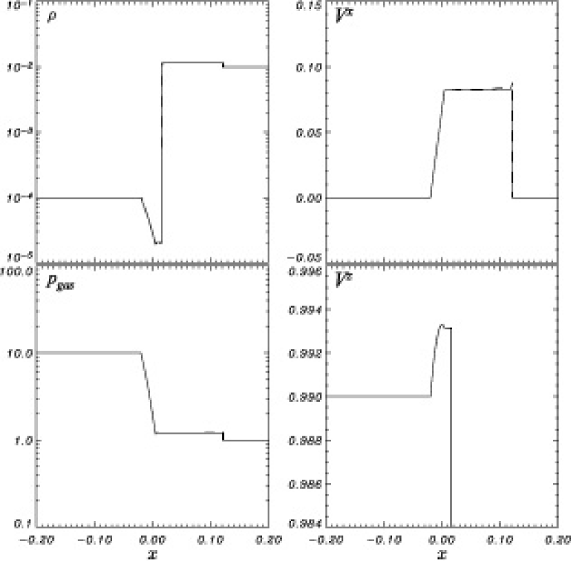
Figure 2: Profiles of (left-upper panel) density, (left-lower panel) gas pressure, (right-upper panel) normal velocity ($v^{x}$), and (right-lower panel) tangential velocity ($v^{z}$) in the HDA case at time $t=0.2$. The solid lines are the exact solution and the dashed lines are the simulation results.

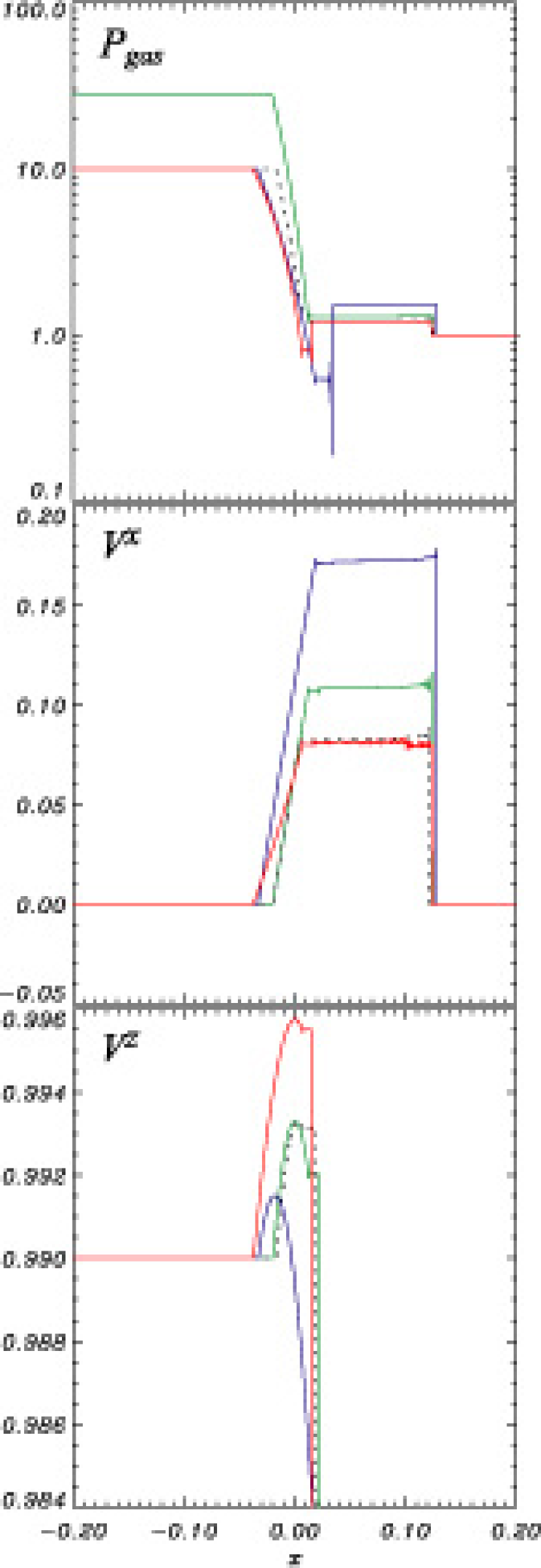
Figure 3: Profiles of gas pressure (upper panel), normal velocity ($v^{x}$) (middle panel), and tangential velocity ($v^{z}$) (lower panel) in the HDB (green), MHDA (blue), MHDB (red), and HDA (dotted-line) cases at time $t=0.2$.

Figure 2 shows the radial profiles of density, gas pressure, velocity normal to the interface ($v^{x}$) - hereafter normal velocity - and velocity tangent to the interface ($v^{z}$)- hereafter tangential velocity - for case HDA. The solution displays a right-moving shock, a right-moving contact discontinuity and a left-moving rarefaction wave (${}_{\leftarrow}RCS_{\rightarrow}$). This hydrodynamical profile is similar to that found by Rezzolla et al. (2003) and Aloy & Rezzolla (2006). The simulation results (dashed lines) are in good agreement with the exact solution (solid lines, calculated with the code of Giacomazzo & Rezzolla 2006) except for the spike in the normal velocity $v^{x}$. Otherwise the normal velocity and propagation of the shock propagating to the right (the forward shock) is $v^{x}\sim 0.082c$ where this value is determined from the exact solution. The small spike evident in Fig. 2 is a numerical artifact and is seen in all simulation results (e.g., in the middle panel of Fig. 3) at the right moving shock ($S_{\rightarrow}$). This numerical spike is reduced by higher resolution calculations (see Appendix A). In the left-moving rarefaction (${}_{\leftarrow}R$) region, the tangential velocity increases as a result of the hydrodynamical boosting mechanism described by Aloy & Rezzolla (2006). In the case shown in Figure 2 the jet is accelerated to $\gamma\sim 12$ from an initial Lorentz factor of $\gamma_{L}\simeq 7$.

Figure 3 displays the resulting profiles of gas pressure, normal velocity ($v^{x}$) and tangential velocity ($v^{z}$) of the magnetohydrodynamic cases MHDA (blue), MHDB (red), and the high pressure, pure-hydrodynamic case HDB (green). In the magnetohydrodynamic cases, the magnetization parameter $\sigma\equiv(B^{{}^{\prime}})^{2}/\rho h$ and the plasma beta parameter $\beta\equiv p_{gas}/p_{mag}$ (on the left side) are 0.556 and 0.45, respectively. The resulting structure consists of a right-propagating fast shock, a right-propagating contact discontinuity, and a left-propagating fast rarefaction wave (${}_{\leftarrow}R_{F}CS_{F\rightarrow}$).

In the MHDA case ($B^{z}=6.0$ ($B^{{}^{\prime}}_{z}=6.0$)) shown as blue curves, the right-moving fast shock ($S_{F\rightarrow}$) and the left-moving fast rarefaction wave (${}_{\leftarrow}R_{F}$) are stronger than the related structures in the HDA case. Consequently, the normal velocity ($v^{x}\sim 0.172c$) is larger than that for the HDA case ($v^{x}\sim 0.082c$). The tangential velocity ($v^{z}\sim 0.9915c$) is lower than that of the HDA case ($v^{z}\sim 0.9933c$). These velocity values are determined from the exact solution. Although the acceleration in the z-direction is weaker, the jet experiences a larger total acceleration than in the HDA case due to the larger normal velocity, and the jet Lorentz factor reaches $\gamma\sim 15$. Thus the “poloidal” magnetic field in the jet region strongly affects sideways expansion, shock profile and total acceleration.

In the MHDB case ($B^{y}=42.0$ ($B^{{}^{\prime}}_{y}=6.0$)) shown as red curves, the right-moving fast shock ($S_{F\rightarrow}$) is slightly weaker than in the HDA case, and the resulting normal velocity ($v^{x}\sim 0.080c$) is slightly less than in the HDA case ($v^{x}\sim 0.082c$). The left-propagating fast rarefaction wave (${}_{\leftarrow}R_{F}$) is stronger than what we found for the HDA case. Therefore the tangential velocity ($v^{z}\sim 0.9958c$) is higher than in the HDA case ($v^{z}\sim 0.9933c$). These velocity values are determined from the exact solution. Altough the “toroidal” magnetic field in the jet region does not greatly affect the sideways expansion and shock profile, the resulting total acceleration to $\gamma\sim 19$ is larger than in the HDA case.

To investigate the effect of the total pressure, we performed a pure-hydrodynamic simulation with high gas pressure (case HDB), shown as green curves, equal to the total (gas plus magnetic) pressure ($p_{tot}=p_{gas}+p_{mag}$) in the MHD cases. The resulting structure for this case is the same as that of HDA case (${}_{\leftarrow}RCS_{\rightarrow}$). The right-moving shock ($S_{\rightarrow}$) and the left-moving rarefaction wave (${}_{\leftarrow}R$) are slightly stronger than those in the HDA case because of the initial high gas pressure in left state. Consequently, the normal velocity $v^{x}$ in the HDB case is larger ($v^{x}\sim 0.108c$) than in the HDA case ($v^{x}\sim 0.0822c$). In the region of the left-propagating rarefaction wave (${}_{\leftarrow}R$), the tangential velocity is the same as that in the HDA case, the jet accelerates only with a marginally greater efficiency than in the HDA case, and the resulting Lorentz factor thus reaches only $\gamma\sim 15$.

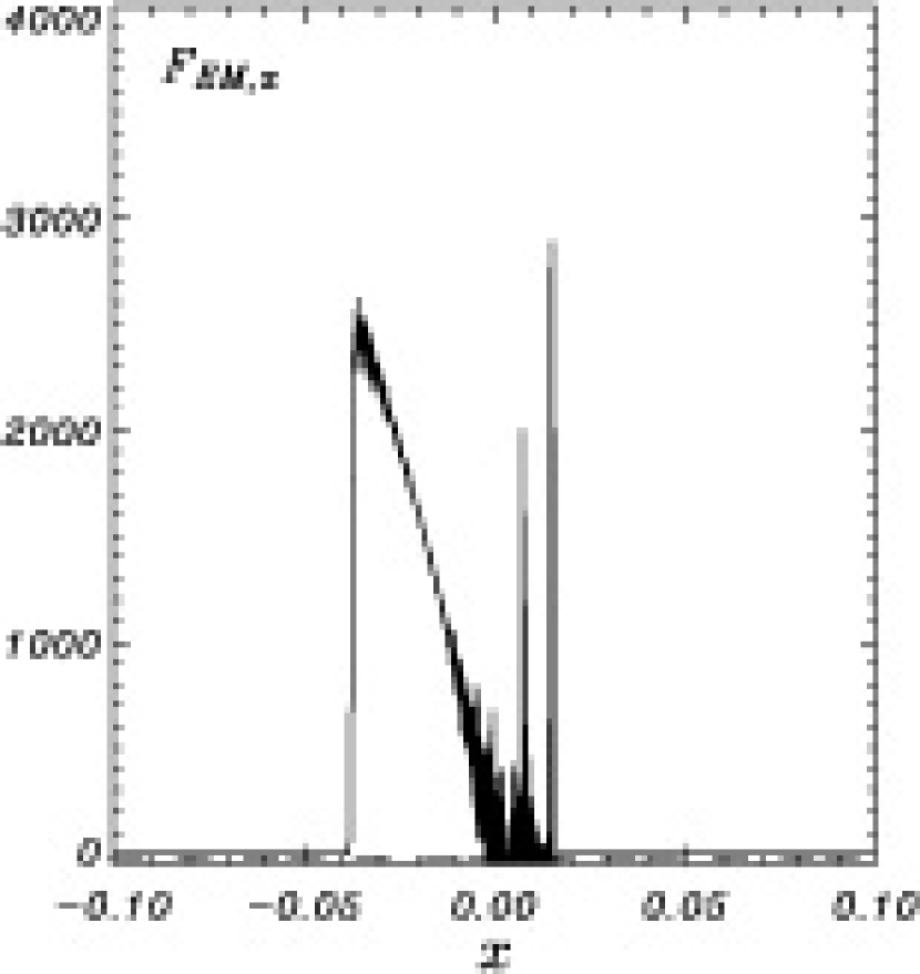
Figure 4: Profile of tangential component of Lorentz force ($F_{EM,z}=(\mathbf{J}\times\mathbf{B})_{z}$) of the MHDA ($B^{{}^{\prime}}_{z}=6.0$)(dashed-line) and the MHDB ($B^{{}^{\prime}}_{y}=6.0$)(solid-line) cases at time $t=0.2$.

Although the total pressure is the same in the hydro HDB case and MHD cases, the existence and direction of the magnetic field changes the shock profiles and acceleration. We summarize the acceleration properties of the different cases in Table 2 where velocity values are determined from the exact solutions. When the gas pressure becomes large in the left state, the normal velocity increases and the jet is more efficiently accelerated. This is because the larger discontinuity in the gas pressure produces a stronger forward shock as well as stronger rarefaction. In MHD, the magnetic pressure is measured in the jet fluid frame and depends on the angle between the flow and magnetic field. The magnetosonic speeds also depend on the angle between the flow and the magnetic field, even for the same magnetic pressure. The direction of the magnetic field is thus a very important geometric parameter for relativistic magnetohydrodynamics. When a “poloidal” magnetic field ($B^{z}$) is present in the jet region, larger sideways expansion is produced, and the jet can achieve higher speed due to the contribution from the normal velocity. By contrast, when a “toroidal” magnetic field ($B^{y}$) is present in the jet region, although the shock profile is only changed slightly, the jet is more accelerated in the tangential direction due to the additional contribution of the tangential component of the Lorentz force ($\mathbf{F}_{EM,z}=(\mathbf{J}\times\mathbf{B})_{z}$) shown in Figure 4 (in the MHDA case there is no additional force). It should be noted that the region with high Lorentz force is approximately coincident with the acceleration region $-0.025$ to $0.0$ and the force still exists at time $t=0.2$. The region with the highest Lorentz force is at the inner edge of the acceleration region. From an efficiency point of view, a “toroidal” magnetic field with the same strength in the jet fluid frame and the same magnetic pressure as those of a “poloidal” field provides the most efficient acceleration. A “poloidal” magnetic field provides acceleration comparable to that resulting from high gas pressure, e.g., the HDB case.

3.2 Dependence of the MHD boost mechanism on magnetic field strength

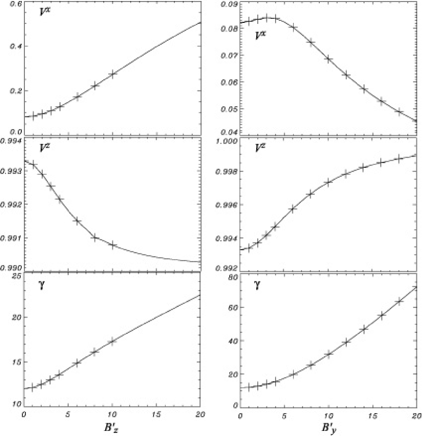
Figure 5: Dependence of maximum normal velocity ($v^{x}$) (upper panel), maximum tangential velocity ($v^{z}$) (middle panels) and maximum Lorentz factor $\gamma=[1-(v^{x})^{2}-(v^{z})^{2}]^{-1/2}$ (lower panels) on the strength of $z$-component of magnetic field $B^{{}^{\prime}}_{z}$ (left panels) and $y$-component of magnetic field $B^{{}^{\prime}}_{y}$ (right panels). The solid line indicates values obtained using the code of Giacomazzo & Rezzolla (2006) and the crosses indicate the values obtained from our simulations at the time $t=0.2$.

To investigate the acceleration efficiency of the magnetic field, we compare jet speeds for the MHDA and MHDB cases and the results are shown in Figure 5. The left panels in Figure 5 show the dependence of the maximum tangential and normal velocities and resulting Lorentz factors on the strength of the poloidal ($B^{{}^{\prime}}_{z}$) component of the magnetic field in the fluid frame. The solid line indicates values obtained using the code of Giacomazzo & Rezzolla (2006) and the crosses indicate values obtained from our simulations at time $t=0.2$. For numerical reasons our code does not yield a solution for $B^{{}^{\prime}}_{z}>10$ ($B^{z}>10$) (the simulation results are indicated by the crosses). When the poloidal magnetic field increases, the code of Giacomazzo & Rezzolla (2006) indicates that the maximum normal velocity increases and the maximum tangential velocity deceases. The break near $B^{{}^{\prime}}_{z}\simeq 4$ occurs near the transition (in the left state) from gas pressure dominated to magnetic pressure dominated. The Lorentz factor results shown in Figure 5 (left bottom panel) indicate that a sufficiently strong poloidal magnetic field in the jet region will allow a jet to achieve $\gamma\sim 22$, even if the jet is only “mildly” relativistic initially, i.e., $\gamma_{L}\sim 7$. We note that in the hydrodynamic cases investigated by Aloy & Rezzolla (2006) the Lorentz factor decreases as the normal velocity increases (see their Fig. 4) where we find that the Lorentz factor increases as the normal velocity increases. Our result is different from that of Aloy & Rezzolla (2006) because their initial conditions were different. In particular, they varied the initial normal velocity in the jet region while holding the initial Lorentz factor constant.

The right panels in Figure 5 show the dependencies of the maximum tangential and normal velocities and the Lorentz factor on the strength of the toroidal ($B^{{}^{\prime}}_{y}$) component of the magnetic field as measured in the jet fluid frame. Again, the solid line indicates values obtained with the code of Giacomazzo & Rezzolla (2006) and the crosses indicate values obtained from our simulations at time $t=0.2$. When the toroidal magnetic field becomes large in the jet region, the maximum normal velocity increases initially, then decreases when $B^{{}^{\prime}}_{y}>4$, and the maximum tangential velocity increases. This dependence is opposite to that of the poloidal magnetic field. The acceleration in the tangential direction occurs due to the additional contribution of the Lorentz force shown in Figure 4. When the toroidal magnetic field becomes large in the jet region, the Lorentz force in the tangential direction increases and contributes to a large acceleration of the jet in the tangential direction. The transition from gas pressure dominated to magnetic pressure dominated left states occurs near $B^{{}^{\prime}}_{y}\simeq 4$. This change from gas to magnetic pressure dominated is reflected in the normal velocity profile. The acceleration is much larger than that found in the comparable poloidal magnetic field case. While at $B^{{}^{\prime}}_{y}\simeq 20$ the maximum Lorentz factor reaches $\gamma\sim 72$, at $B^{{}^{\prime}}_{z}\simeq 20$ the maximum Lorentz factor is only $\gamma\sim 22$.

3.3 Multidimensional simulations

To investigate the effects induced by more than one degree of freedom, we perform two dimensional RMHD simulations of the MHDA case ($B^{{}^{\prime}}_{z}=6.0$). The computational domain corresponds to a local part of the jet flow. In the simulations, a “pre-existing” jet flow is established across the computational domain. The initial condition is the same as that of the 1D MHDA case (e.g., $v^{z}=0.99c$ and $B^{{}^{\prime}}_{z}=6.0$). In order to investigate a possible influence of the chosen coordinate system, we perform the calculations in Cartesian and cylindrical coordinates. The discontinuities between the jet and the external medium are set at $x$ or $r=1.0$ in the initial state (see Fig. 1). The computational domain is $0.5\leq x,r\leq 1.5$ and $0\leq z\leq 5.0$ with $(N_{x,r}\times N_{z})=(2000\times 250)$, where $N_{x,r}$ and $N_{z}$ are the number of computational zones in the $x$ or $r$ direction and in the $z$ direction. We use a large number of computational zones in the $x$ or $r$ direction in order to satisfactorily resolve the shock profile. We impose periodic boundary conditions in the z-direction and free boundary conditions in the $x$ or $r$ direction. The computational domain is far from the jet center in order to obtain high resolution near the jet surface. In this case it is necessary to use free boundary conditions at the inner boundary in $x$ or $r$. Here we are far from the jet axis and waves and fluid must be free to move towards the axis through this boundary and not experience a reflection.

The initial condition for these 2D simulations is a simple extension of the 1D MHDA case into the z-direction and represents the temporal development of a planar (Cartesian coordinates) or cylindrical interface that is infinite in extent in the z-direction. Effectively we consider a local part of a jet flow. Here we consider only the poloidal magnetic field case as a uniformly overpressured cylindrical jet containing a uniform poloidal magnetic field as valid physically. The “toroidal” magnetic field case in 1D cannot be compared to a proper cylindrical toroidal magnetic field in which hoop stresses and radial gradients will play a role.

Figure 6 shows 2D images of the Lorentz factor for the 2D MHDA simulation in Cartesian and in cylindrical coordinates at time $t=0.6$. The left-moving rarefaction waves do not reach the inner boundary ($x$ or $r$ direction) so the choice of inner outflow boundary condition does not influence the results. In both cases, a thin surface is accelerated by the MHD boost mechanism to reach a maximum Lorentz factor $\gamma\simeq 15$ from an initial Lorentz factor $\gamma_{L}\simeq 7$. The jet in cylindrical coordinates is slightly more accelerated than the jet in Cartesian coordinates. The presence of velocity shear between the jet and external medium can excite Kelvin-Helmholtz (KH) instabilities (e.g., Ferrari et al. 1978; Hardee 1979, 1987, 2000; Birkinshaw 1984), and such instability might affect the relativistic boost mechanism. However, we do not see any growth of the KH instability during the simulation. This is because the simulation duration is too short for KH instabilities to grow. However, in longer duration RMHD cylindrical jet simulations KH instabilities can grow (Hardee 2007; Mizuno et al. 2007) and this might effect significantly the later stages of jet evolution.

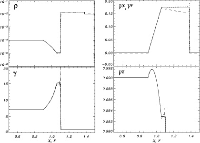
Figure 7: Profiles of (left-upper panel) density, (left-lower panel) Lorentz factor, (right-upper panel) normal velocity ($v^{x},v^{r}$), and (right-lower panel) tangential velocity ($v^{z}$) of the 2D MHDA case in Cartesian coordinates (dotted lines) and the 2D MHDA case in cylindrical coordinates (dashed lines) at time $t=0.6$. The solid lines are the exact solution of the 1D MHDA case at time $t=0.6$.

In order to investigate simulation results quantitatively, we have taken one-dimensional cuts through the computational box perpendicular to the z-axis. Figure 7 shows the resulting profiles of gas pressure, Lorentz factor ($\gamma$), normal velocity ($v^{x}$ or $v^{r}$) and tangential velocity ($v^{z}$) of the 2D MHDA cases in Cartesian (dotted lines) and in cylindrical coordinates (dashed lines). The exact solution of the 1D MHDA case is shown as solid lines. The result consists of a right-moving fast shock, right-moving contact discontinuity, and a left-moving fast rarefaction wave (${}_{\leftarrow}R_{F}CS_{F\rightarrow}$). The profiles from the 2D MHDA simulation in Cartesian coordinates match well those of the 1D MHDA case. In the 2D MHDA simulation with cylindrical coordinates, the right-moving fast shock ($S_{F\rightarrow}$) is weaker and the left-moving fast rarefaction wave (${}_{\leftarrow}R_{F}$) is slightly stronger than those of the 2D MHDA simulation with Cartesian coordinates. Selecting cylindrical coordinates, causes the normal velocity to decrease gradually in the expansion. The tangential velocity in cylindrical coordinates ($v^{z}\sim 0.991530c$) is slightly faster than in Cartesian coordinates ($v^{z}\sim 0.991500c$). Thus the jet Lorentz factor reaches $\gamma\sim 16$ in cylindrical coordinates and $\gamma\sim 15$ in Cartesian coordinates. This result suggests that different coordinate systems affect sideways expansion, shock profile, and acceleration slightly.

4 Summary and Discussion

We performed relativistic magnetohydrodynamic simulations of an acceleration boosting mechanism for fast astrophysical jet flows that results from highly overpressured, tenuous flows with an initially modest relativistic speed relative to a colder, denser external medium at rest. We employed the RAISHIN code (Mizuno et al. 2006a), to study the relativistic boost mechanism proposed by Aloy & Rezzolla (2006), who showed that hydrodynamic accelerations to $\gamma>1000$ are possible in the situation described above. For numerical reasons, we reduced the pressure discontinuity between the hotter higher pressure jet and colder lower pressure external medium and also reduced the initial jet velocity (see Apendix A3). Our results still show the same behavior (${}_{\leftarrow}RCS_{\rightarrow}$) found in Rezzolla et al. (2003) and Aloy & Rezzolla (2006). The same hydrodynamical structures emerge in our simulation, confirming the basic properties of the boost mechanism proposed in their work. Subsequently we extended their investigation to study the effects of magnetic fields that are parallel (poloidal) and perpendicular (toroidal) to the flow direction but parallel to the interface.

Our simulations show that the presence of a magnetic field in the jet can significantly change the properties of the outward moving shock and inward moving rarefaction wave, and can in fact result in even more efficient acceleration of the jet than in a pure-hydrodynamic case. In particular, the presence of a toroidal magnetic field perpendicular to jet flow produces a stronger inward moving rarefaction wave. This leads to acceleration from $\gamma\sim 7$ to $\gamma\gtrsim 15$ when the magnetic pressure is comparable to the gas pressure. A comparable pure-hydrodynamic case yields acceleration to $\gamma\lesssim 12$. Our results would indicate acceleration to $\gamma\sim 100$ for a case with magnetic pressure 40 times the gas pressure. Thus, the magnetic field can in principle play an important role in this relativistic boost mechanism.

We found that a jet with a flow aligned poloidal field was slightly more accelerated in cylindrical coordinates than one in Cartesian coordinates but in general our 1D and 2D results for the poloidal field appear comparable. The current simple 2D MHD simulation in cylindrical coordinates is directly applicable to a 3D cylindrical geometry where the magentic field and jet flow are aligned and tangent to the jet-external medium interface. However, recent GRMHD simulations of jet formation predict that the jet has a rotational velocity and considerable radial structure (e.g., Nishikawa et al. 2005; Mizuno et al. 2006b; De Villiers et al. 2005; Hawley & Krolik 2006; McKinney & Gammie 2004; McKinney 2006). The effect of such radial structure on this boost mechanism is yet to be determined.

Our present results for the 1D “toroidal” field are not likely to apply in a 3D cylindrical geometry where a toroidal field exerts a hoop stress that does not exist in the 1D configuration. It seems likely that this hoop stress would so modify the sideways expansion of an overpressured cylindrical jet as to render our present toroidal field results not applicable unless the magnetic field in 3D is tangled or the thin boost region is relatively insensitive to radial gradients. In order to properly investigate full 3D effects, it will be necessary to perform full 3D RMHD simulations including toroidal and helical magnetic fields.

The initial conditions in our present 2D simulations are a simple extension of the 1D poloidal MHD case, models a local part of an overpressured jet flow in a colder denser ambient and provides a first step toward multi dimensional simulations. To address the question whether or not such strong, magnetically enhanced boosts really do take place in astrophysical sources (AGNs, quasars, microquasars, gamma-ray bursts) will require additional numerical simulations to show that this process can work for jets injected into a reasonable astrophysical environment. The operation of the MHD boost is likely to be strongly affected by the properties of the external medium, expected jet overpressures, and spatial development of the jet flow and external medium downstream from the jet source. For example, it is conceivable that magnetic pressure effects are more dominant relative to thermal pressure effects in AGN jets where a magnetically dominated “Poynting” flux jet is confined by a colder, denser external medium. A hot GRB fireball can expand and accelerate under its thermal pressure to reach large Lorentz factors as long as baryon-loading is small (Mészáros et al. 1993; Piran et al. 1993). Although this simple model can account for the large ($>100$) Lorentz factors inferred for GRBs, it does not reflect more realistic settings of complex GRB progenitor/central engine models. In the collapsar model for long-duration GRBs (Woosley 1993), the tenuous jet is believed to propagate in a surrounding dense stellar envelope (Zhang et al. 2003), so that the hydrodynamic configuration considered by Aloy & Rezzolla (2006) and in this paper is naturally satisfied. A strong poloidal magnetic field is likely present at the central engine. In some GRB models, the flow is even dominated by a Poynting flux (Lyutikov 2006). In this case the magnetohydrodynamic boost mechanism discussed here would then play an important role in jet acceleration. The final Lorentz factor should depend on the detailed parameters invoked in this mechanism as well as the unknown baryon loading process during the propagation of the jet in the envelope. In the case of short GRBs that may be of compact star merger origin (e.g., Paczýnski 1986; Nakar 2007), there is no dense stellar envelope surrounding the jet. The jet region is nonetheless more tenuous than the surrounding medium due to the centrifugal barrier in the jet, so that the acceleration mechanism discussed here still applies (e.g., see Aloy et al. 2005 for the pure hydrodynamic case). Due to a likely smaller baryon loading in the merger environment, the jet may achieve an even higher Lorentz factor than for the case of long GRBs, as suggested by some observations (e.g. their harder spectrum and shorter spectral lags). The magnetohydrodynamic acceleration mechanism discussed here also naturally yields a GRB jet with substantial angular structure. In particular, since acceleration is favored in the rarefaction region near the contact discontinuity, this mechanism naturally gives rise to the kind of ring-shaped jet that has been discussed in some empirical GRB models (e.g. Eichler & Levinson 2006).

Appendix A Resolution Tests

A.1 One-dimensional shock tube tests with transverse velocity

Recently it has been reported that it is numerically challenging to resolve 1D shock tube test problems with transverse velocities using the same number of computational zones used in the absence of transverse velocities (Mignone & Bodo 2005; Zhang & MacFadyen 2006; Mizuta et al. 2006). We have performed a resolution study using from 800 to 12,800 uniform zones spanning $L_{x}=1.0$, where $L_{x}$ is the simulation size in the x direction, and we have used the initial conditions from Mignone & Bodo (2005) and Mizuta et al. (2006) with adiabatic index $\Gamma=5/3$ as follows:

Left state $(0<x<0.5)$: $\rho_{L}=1.0$, $p_{L}=1.0\times 10^{3}$, $v^{x}_{L}=0$, $v^{z}_{L}=0.9~{}c$.

Right state $(0.5<x<1.0)$: $\rho_{R}=1.0$, $p_{R}=1.0\times 10^{-2}$, $v^{x}_{R}=0$, $v^{z}_{R}=0$.

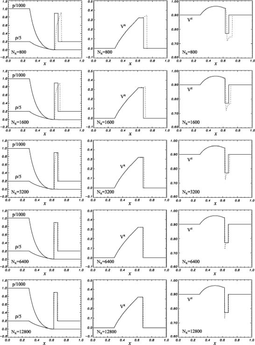
Figure 8: Profiles of the shock tube test problem with a transverse velocity at time $t=0.4$. The solid lines are the exact solution and the dotted lines are the simulation results. Different simulation resolutions are presented; the number of computational zones ($N_{x}$) is 800, 1600, 3200, 6400, and 12,800 from top to bottom. The density, gas pressure, normal velocity ($v^{x}$) and tangential velocity ($v^{z}$) are shown.

The results of numerical and analytical solutions to this test problem are shown in Figure 8. The left-going rarefaction (${}_{\leftarrow}R$) is resolved with good accuracy even at lower resolution. On the contrary, both right-going shock and contact discontinuities ($CS_{\rightarrow}$) are not resolved in both position and value in lower resolution calculations. In calculations with higher resolution (typically $N_{x}\geq 6400$ over $L_{x}=1.0$) the shock front position is calculated correctly. However, there still remains some undershoot in $v^{z}$ at the contact discontinuity.

A.2 One dimensional hydrodynamic relativistic boost model

We also performed a resolution study of the HDA case. The initial condition is described in Table 1. The simulations have been performed using from 800 to 12,800 uniform zones spanning $L_{x}=0.4$ equivalent to using 2000 to 32,000 uniform zones spanning $L_{x}=1.0$.

The results of numerical and analytical solutions are shown in Figure 9. The left-going rarefaction (${}_{\leftarrow}R$) is resolved to good accuracy at even the lowest resolution. On the other hand, the right-going shock ($S_{\rightarrow}$) is not sufficiently resolved in both position and value in lower resolution calculations. Higher resolution calculations ($N_{x}\geq 6400$) determine the shock front position with good accuracy. However, there still remains some overshoot in $v^{x}$ behind the right-going shock.

We conclude from this study that the use of 6400 computational zones spanning $L_{x}=0.4$ used for our 1D simulations provides excellent quantitative accuracy. The use of 2000 computational zones spanning $L_{x}=1.0$, equivalent to 800 zones spanning $L_{x}=0.4$, provides sufficient quantitative accuracy for the comparison between 1D and 2D results.

A.3 One dimensional hydrodynamic relativistic boost model (Aloy & Rezzolla model)

We have performed a resolution study of the one dimensional hydrodynamic relativistic boost model proposed by Aloy & Rezzolla (2006). The simulations have been performed using from 800 to 12,800 uniform zones spanning $L_{x}=0.4$. Here we have used the initial density and pressure conditions in the left and right states with adiabatic index $\Gamma=5/3$ from Aloy & Rezzolla (2006) but with a reduced tangential velocity as follows:

Left state $(-0.2<x<0.0)$: $\rho_{L}=1.0\times 10^{-4}$, $p_{L}=1.0\times 10^{-3}$, $v^{x}_{L}=0$, $v^{z}_{L}=0.99~{}c$.

Right state $(0.0<x<0.2)$: $\rho_{R}=1.0\times 10^{-2}$, $p_{R}=1.0\times 10^{-6}$, $v^{x}_{R}=0$, $v^{z}_{R}=0$.

The results of numerical and analytical solutions are shown in Figure 10. The left-going rarefaction (${}_{\leftarrow}R$), right-going contact discontinuity and shock ($CS_{\rightarrow}$) are not sufficiently resolved in both position and value in lower resolution calculations. Higher resolution calculations ($N_{x}>6400$) determine the position and value of the left-going rarefaction wave with good accuracy. However, even in the highest resolution calculation ($N_{x}=12,800$) still the right-going contact discontinuity and shock are not resolved. We conclude from this study that in order to resolve the Aloy & Rezzolla model with good accuracy we would have to perform simulations with much higher resolution and employ the Adaptive Mesh Refinement method like that used by Zhang & MacFadyen (2006) to obtain locally higher resolution at the area where shocks and contact discontinuities exist to save CPU time and memory.

Table 1: Model and Parameters

Case		$\rho$	$p$	$v^{x}$	$v^{y}$	$v^{z}$	$B^{x}(B^{{}^{\prime}}_{x})$	$B^{y}(B^{{}^{\prime}}_{y})$	$B^{z}(B^{{}^{\prime}}_{z})$
HDA	left state	$10^{-4}$	10.0	0.0	0.0	0.99	0.0(0.0)	0.0(0.0)	0.0(0.0)
	right state	$10^{-2}$	1.0	0.0	0.0	0.0	0.0(0.0)	0.0(0.0)	0.0(0.0)
HDB	left state	$10^{-4}$	28.0	0.0	0.0	0.99	0.0(0.0)	0.0(0.0)	0.0(0.0)
	right state	$10^{-2}$	1.0	0.0	0.0	0.0	0.0(0.0)	0.0(0.0)	0.0(0.0)
MHDA	left state	$10^{-4}$	10.0	0.0	0.0	0.99	0.0(0.0)	0.0(0.0)	6.0(6.0)
	right state	$10^{-2}$	1.0	0.0	0.0	0.0	0.0(0.0)	0.0(0.0)	0.0(0.0)
MHDB	left state	$10^{-4}$	10.0	0.0	0.0	0.99	0.0(0.0)	42.0(6.0)	0.0(0.0)
	right state	$10^{-2}$	1.0	0.0	0.0	0.0	0.0(0.0)	0.0(0.0)	0.0(0.0)

Note. — HDA is a hydrodynamic case. MHDA and MHDB are magnetohydrodynamic cases with $B^{z}_{L}=6.0$ ($B^{{}^{\prime}}_{z,L}=6.0$) and $B^{y}_{L}=42.0$ ($B^{{}^{\prime}}_{y,L}=6.0$) respectively. HDB is a hydrodynamic case with gas pressure $p_{gas,L}$ equal to $p_{tot,L}=p_{gas,L}+p_{mag,L}$ in the MHD cases.

Table 2: Maximum velocities and Lorentz factor

Case	$v^{x}$	$v^{z}$	$\gamma$
HDA	0.082211	0.993292	11.9820
HDB (high gas pressure)	0.107550	0.993293	15.2890
MHDA (poloidal field)	0.171533	0.991502	14.8255
MHDB (toroidal field)	0.080350	0.995750	19.9020

Note. — Velocity values determied from exact solutions.

Figure 6: 2D images of the Lorentz factor showing the (a) initial condition, (b) results of the 2D MHDA case in Cartesian coordinates and (c) results of the 2D MHDA case in cylindrical coordinates at time $t=0.6$. The color scales show the Lorentz factor. Arrows depict the poloidal velocities normalized to light speed.

Figure 9: Profiles of the HDA case at time $t=0.2$. The solid lines are the exact solution and the dotted lines are the simulation results. Different simulation resolutions are presented; the number of computational zones ($N_{x}$) is 800, 1600, 3200, 6400, and 12,800 from top to bottom. The density, gas pressure, normal velocity ($v^{x}$) and tangential velocity ($v^{z}$) are shown.

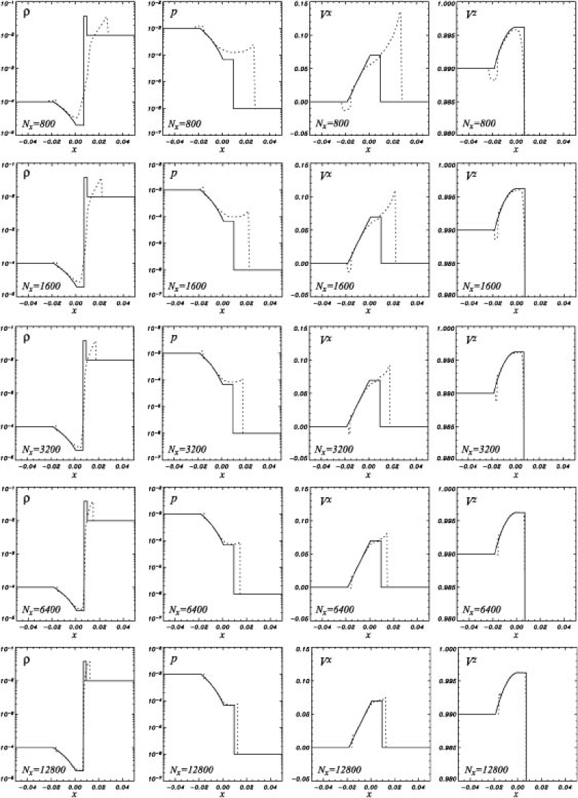
Figure 10: Profiles of hydrodynamic relativistic boost model proposed by Aloy & Rezzolla (2006) at time $t=0.2$. The solid lines are the exact solution and the dotted lines are the simulation results. Different simulation resolutions are presented; the number of computational zones ($N_{x}$) is 800, 1600, 3200, 6400, and 12,800 from top to bottom. The density, gas pressure, normal velocity ($v^{x}$) and tangential velocity ($v^{z}$) are shown.

References

- Aloy et al. (2005) Aloy, M. A., Janka, H.-T. & Müller, E. 2005, A&A, 436, 273
- Aloy & Rezzolla (2006) Aloy, M. A. & Rezzolla, L. 2006, ApJ, 640, L115
- Balbus&Hawley (1991) Balbus, S. A., and Hawley, J. F. 1991, ApJ 376, 214
- Balbus&Hawley (1998) Balbus, S. A., and Hawley, J. F. 1998, Rev. Mod. Phys. 70, 1
- Birkinshaw (1991) Birkinshaw, M. 1991, MNRAS, 252, 505
- Blandford & Znajek (1977) Blandford, R. D. & Znajek, R. L. 1977, MNRAS, 179, 433
- Blandford & Payne (1982) Blandford, R. D. & Payne, D. G. 1982, MNRAS, 199, 883
- De Villiers et al. (2005) De Villiers, J.-P., Hawley, J. F., Krolik, J. H., & Hirose, S. 2005, ApJ, 620, 878
- Drenkhahn & Spruit (2002) Drenkhahn, G., & Spruit, H. C. A&A, 391, 1141
- Eichler & Levinson (2006) Eichler, D. & Levinson, A. 2006, ApJ, 649, L5
- Ferrari (1998) Ferrari, A. 1998, ARA&A, 36, 539
- Ferrari et al. (1978) Ferrari, A., Trussoni, E., & Zaninetti, L. 1978, A&A, 64, 43
- Fukue (1990) Fukue, J. 1990, PASJ, 42, 793
- Giacomazzo & Rezzolla (2006) Giacomazzo, B. & Rezzolla, L. 2006, J. Fluid Mech., 562, 223
- Hardee (1979) Hardee, P. E. 1979, ApJ, 234, 47
- Hardee (1987) —–. 1987, ApJ, 318, 78
- Hardee (2007) —–. 2007, ApJ, 664, 26
- Harten et al. (1983) Harten, A., Lax, P. D., & van Leer, B. J. 1983, SIAM Rev., 25, 35
- Hawley & Krolik (2006) Hawley & Krolik 2006, ApJ, 614, 103
- Koide et al. (1999) Koide, S., Shibata, K., Kudoh, T. 1999, ApJ, 522, 727
- Koide et al. (2000) Koide, S., Meier, D. L., Shibata, K., & Kudoh, T. 2000, ApJ, 536, 668
- Lyutikov (2006) Lyutikov, M. 2006, New J. Phys., 8, 119
- McKinney (2006) McKinney, J. C. 2006, MNRAS, 368, 1561
- McKinney & Gammie (2004) McKinney, J. C. & Gammie, C. F. 2004, ApJ, 611, 977
- Mészáros (2006) Mészáros, P. 2006, Rep. Prog. Phys., 69, 2259
- Mészáros et al (2003) Mészáros, P., Laguna, P. & Rees, M. J. 1993, ApJ, 415, 181
- Mignone & Bodo (2005) Mignone, A., & Bodo, G. 2005, MNRAS, 364, 126
- Miller et al. (2006) Miller, J. M., et al. 2006, Nature 441, 953
- Mirabel & Rodríguez (1999) Mirabel, I. F. & Rodríguez, L. F. 1999, ARA&A, 37, 409
- Mizuno et al. (2006a) Mizuno, Y., Nishikawa, K.-I., Koide, S., Hardee, P., & Fishman, G. J. 2006a, ApJS, submitted (astro-ph/0609004)
- Mizuno et al. (2006b) —–. 2006b, PoS, MQW6,045
- Mizuno et al. (2007) Mizuno, Y., Hardee, P., & Nishikawa, K.-I., 2007, ApJ, 662, 835
- Mizuta et al. (2006) Mizuta, A., Yamasaki, T., Nagataki, S., & Mineshige, S. 2006, ApJ, 651, 960
- Nakar (2007) Nakar, E. 2007, Phys. Rep., 442, 166
- Nishikawa et al. (2005) Nishikawa, K.-I., Richardson, G., Koide, S., Shibata, K., Kudoh, T., Hardee, P., & Fishman, G. J. 2005, ApJ, 625, 60
- Noble et al. (2006) Noble, S. C., Gammie, C. F., McKinney, J. C., & Del Zanna, L. 2006, ApJ, 641, 626
- Paczynski (1986) Paczýnski, B. 1986, ApJ, 308, L43
- Penrose (1969) Penrose, R. 1969, Nuovo Cimento, 1, 252
- Piran (2005) Piran, T. 2005, Reviews of Modern Physics, 76, 1143
- Piran (1993) Piran, T., Shemi, A. & Narayan, R. 1993, MNRAS, 263, 861
- Rezzolla et al. (2003) Rezzolla, L., Zanotti, O., & Pons, J. A. 2003, J. Fluid Mech., 479, 199
- Stephens et al. (2006) Stephens, B. C., Duez, M. D., Liu, Y. T., et al. (2007), Class. Quantum Grav., 24, 207
- Tóth (2000) Tóth, G. 2000, J. Comput. Phys., 161, 605
- Urry & Padovani (1995) Urry, C. M. & Padovani, P. 1995, PASP, 107, 803
- Woosley (1993) Woosley, S. E. 1993, ApJ, 405, 273
- Woosley and janka (2005) Woosley, S. E., and Janka, H.-T. 2006, Nature Physics, 1, 147
- Zhang & Mészáros (2004) Zhang, B. & Mészáros, P. 2004, Int. J. Mod. Phys., A19, 2385
- Zhang & MacFadyen (2006) Zhang, W., & MadFadyen, A. I. 2006,ApJS, 164, 255
- Zhang et al. (2003) Zhang, W., Woosley, S. E. & MacFadyen, A. I. 2003, ApJ, 586, 356