Feynman integrals and difference equations

Abstract:

We report on the calculation of multi-loop Feynman integrals for single-scale problems by means of difference equations in Mellin space. The solution to these difference equations in terms of harmonic sums can be constructed algorithmically over difference fields, the so-called $\Pi\Sigma^{*}$-fields. We test the implementaion of the Mathematica package Sigma on examples from recent higher order perturbative calculations in Quantum Chromodynamics.

1 Introduction

In quantum field theory the perturbative calculation of a given scattering amplitude or cross section requires the evaluation of Feynman diagrams. Especially at higher orders this is a difficult task and over the last years, a large variety of methods has been devised to deal with the problem of calculating Feynman integrals, see e.g. [1] and references therein. The necessary integration over the propagators of the virtual or unobserved particles are typically carried out in momentum space and divergent integrals are regularized dimensionally by shifting from 4 to $D=4-2\epsilon$ dimensions of space-time. For a given Feynman integral the main task is then the derivation of an analytical expression in terms of known functions with well-defined properties, which at the same time permits a Laurent expansion in the small parameter $\epsilon=(D-4)/2$.

In these proceedings we want to focus on particular progress in this direction through the systematic and efficient approach to solve difference equations. To that end, we start by briefly stating the physics case and present the necessary mathematical definitions. Then we provide explicit examples from recent higher order perturbative calculations in Quantum Chromodynamics (QCD) and finish with a summary and an outlook.

1.1 Setting the stage

For a given scattering process the Feynman integrals are classified by the number $n$ of external legs ($n$-point functions), by the number of independent loops $l$ and by the topology of the associated graph. Initially, the Feynman integrals will appear as tensor integrals $I^{\mu_{1},\mu_{2},\dots}$ where $\mu_{i}$ denote Lorentz indices. Subsequently tensor integrals can be mapped to scalar integrals by numerous methods, thus we are dealing with expressions

$$I(D;\nu_{1},\dots,\nu_{n})\,=\,\int\,d^{D}p_{1}\,\dots\,d^{D}p_{l}\,{1\over(p_{1}^{2}-m_{1}^{2})^{\nu_{1}}\,\dots\,(p_{n}^{2}-m_{n}^{2})^{\nu_{n}}}\,,$$ (1)

where the momenta $p_{i}$, $i=l+1,\dots,n$, are related by energy-momentum conservation $p_{i}=f(p_{1},\dots,p_{l})$, and $m_{i}$ denote the masses of the associated particles. The powers of the propagators are $\nu_{i}$ and $D$ is the (complex) space-time dimension. In the most general case Feynman integrals such as in Eq. (1) may depend on multiple scales, for instance the masses $m_{i}$ but also the non-vanishing scalar products of external momenta.

In the following, we will focus on perturbative calculations to higher orders in massless QCD for single-particle inclusive observables. These depend on a single scaling variable $x$ only, with $x\in[0,1]$. Prominent examples are structure functions in deep-inelastic scattering (DIS), fragmentation functions in electron-positron ($e^{+}e^{-}$) annihilation or the total cross sections for the Drell-Yan process or Higgs production at hadron colliders. All these quantities can be solved directly and systematically in Mellin $N$-space, an approach that has been used in the past within the framework of the operator product expansion (and exploiting the optical theorem) in DIS [2, 3]. More recently, also innovative extensions to other kinematics have been considered [4]. For a generic observable ${\cal O}(x)$, we can write

$${\cal O}(N) \!=\! \int_{0}^{1}dx\,x^{N-1}{\cal O}(x)$$ (2)

$$\!=\! \int_{0}^{1}dx\,x^{N-1}\int{\rm dPS}^{(m)}\bigl{|}M(\{\mbox{in}\}\to\{\mbox{out}\})\bigr{|}^{2}\delta(x-f)$$

$$\!=\! \int{\rm dPS}^{(m)}\bigl{|}M(\{\mbox{in}\}\to\{\mbox{out}\})\bigr{|}^{2}{1\over f^{-N+1}}\,,$$

where the first line defines the Mellin transform. Subsequently, we express ${\cal O}(x)$ through the square of the scattering amplitude $M(\{\mbox{in}\}\to\{\mbox{out}\})$ for a given set of incoming and outgoing particles and ${\rm dPS}^{(m)}$ denotes the integration measure of the Lorentz invariant phase space. The invariant $f$ depends on internal and external momenta and introduces the Mellin-$N$ dependence. As an upshot, the observables are mapped to a discrete set of variables (positive integer Mellin $N$).

Once the steps in Eq. (2) are accomplished, the scalar integrals can be reduced algebraically to so-called master integrals. The reduction algorithms are based on integration-by-parts, see e.g. [1],

$$0\,=\,\int\,d^{D}p_{1}\,\dots\,d^{D}p_{l}\,\left({p_{i}}_{\mu}{\partial\over\partial p_{j}^{\mu}}\right)\,{1\over(p_{1}^{2})^{\nu_{1}}\,\dots\,(p_{n}^{2})^{\nu_{n}}}\,{1\over f^{-N+1}}\,,$$ (3)

where $p_{i}$ and $p_{j}$ denote any of the loop momenta and the Mellin-$N$ dependence is implicit through the invariant $f$, cf. Eq. (2). Upon resolving the constraints from $f$ the reductions in Mellin space act on monomials like $(p_{i}^{2})^{-\nu_{i}+N}$ and give rise to systems of linear equations which can be solved in terms of a (small) set of master integrals. This step is automatized by using suitable (customized) computer algebra programs although in practice limitations arise at higher orders through the excessively large size of the systems of linear equations which need to be considered.

Due to the explicit dependence on the Mellin variable $N$ the master integrals themselves are functions of $N$. Their functional dependence on $N$ is completely determined by the difference equations they satisfy. These difference equations in $N$ are obtained as well from the solutions to the integration-by-parts reductions and they are the central topic of the present proceedings.

With the help of Eq. (2) and the solutions to the integration-by-parts reductions, we are thus in a position to express a given Feynman integral $I(N)$ in Mellin space in a recursive manner,

$$a_{0}(N)I(N)+a_{1}(N)I(N-1)+\dots+a_{k}(N)I(N-k)\,=\,X(N)\,,$$ (4)

which defines a difference equation of order $k$ with the parametric dependence on $\epsilon$ being implicit in Eq. (4). The functions $a_{i}(N)$ are polynomials in $N$ (and $\epsilon$), sometimes they factorize linearly in terms of the type $N+m+n\epsilon$ with integer $m,n$. $X(N)$ denotes the inhomogeneous part which collects the simpler integrals and in a Laurent series in $\epsilon$ it is typically composed of harmonic sums $S_{\vec{m}}$ (${\vec{m}}=m_{1},\dots,m_{k}$) of weight $w=|m_{1}|+\dots+|m_{k}|$ and, possibly, in combination with values of the $\zeta$-function and powers of $N$.

From a practical view-point in quantum field theory, an approach like Eq. (4) allows for easy checking at fixed values of the Mellin moment $N$. The analytical solution to Eq. (4) requires concepts and algorithms of symbolic summation (discussed e.g. in [5]) and has been possible in all cases we have encountered in QCD calculations [6, 7, 8, 9]. However, the recurrence relations can also be embedded in a mathematical framework, to which we will turn in the following.

2 Solving recurrence relations in difference fields

The Mellin space approach to Feynman integrals at higher orders which we have briefly sketched above leads us to the following key problem:

Given sequences $a_{0}(k),\dots,a_{m}(k)$ and $f_{1}(k),\dots,f_{d}(k)$, find all constants $c_{1},\dots,c_{d}$, free of $k$, and all $g(k)$ such that the parameterized linear difference equation

$$a_{m}(k)g(k+m)+a_{m-1}(k)g(k+m-1)+\dots+a_{0}(k)g(k)=c_{1}f_{1}(k)+\dots+c_{d}f_{d}(k)$$ (5)

holds.

Note that this problem covers various prominent subproblems. Specializing to $d=1$, this is nothing else than recurrence solving, i.e. we are back to Eq. (4). Taking $m=1$ with $a_{0}=-1$ and $a_{1}=1$ we get parameterized telescoping; in particular, given a bivariate sequence $f(n,k)$, one can set $f_{i}(k):=f(n+i-1,k)$ which corresponds in the hypergeometric case to Zeilberger’s creative telescoping [10]. Finally, choosing $d=m=1$ with $a_{0}=-1$, $a_{1}=1$, we arrive at telescoping; for more details and applications of these summation principles see [11].

The algorithmic solution of Eqs. (4) or (5) requires algorithms for symbolic summation which are typically implemented in computer algebra systems like Maple, Mathematica or Form [12], the latter being most advantageous if large expressions are involved. Specific implementations that deal with symbolic summation are e.g. Summer [13] or the recent summation package Sigma [14], which can handle problem (5), and therefore telescoping, creative telescoping and recurrence solving, if the $a_{0},\dots,a_{m}$ and $f_{1},\dots,f_{d}$ are given by expressions in terms of indefinite nested sums and products. More precisely, Sigma translates such sum–product expressions into difference fields, the so-called $\Pi\Sigma^{*}$-fields, and solves the given problem (5) there.

2.1 The construction of difference fields

Given an equation of the form (5), one can represent the coefficients $a_{i}$ and the inhomogeneous parts $f_{i}$ in the so-called $\Pi\Sigma^{*}$-fields [15].

Definition. Let $\mathbb{F}$ be a field with characteristic $0$ and let $\sigma$ be a field automorphism of $\mathbb{F}$. Then $(\mathbb{F},\sigma)$ is called a difference field; the constant field of $\mathbb{F}$ is defined by ${\rm const}_{\sigma}{\mathbb{F}}=\{f\in\mathbb{F}|\sigma(f)=f\}$. A difference field $(\mathbb{F},\sigma)$ with constant field $\mathbb{K}$ is called a $\Pi\Sigma^{*}$-field if $\mathbb{F}=\mathbb{K}(t_{1},\dots,t_{e})$ where for all $1\leq i\leq e$ each $\mathbb{F}_{i}=\mathbb{K}(t_{1},\dots,t_{i})$ is a transcendental field extension of $\mathbb{F}_{i-1}=\mathbb{K}(t_{1},\dots,t_{i-1})$ and $\sigma$ has the property that $\sigma(t_{i})=a\,t_{i}$ or $\sigma(t_{i})=t_{i}+a$ for some $a\in\mathbb{F}_{i-1}$.

Remark. In order to transform, e.g., nested sums in such $\Pi\Sigma^{*}$-fields, one exploits the following important fact. Suppose we are given a sum $T(n)=\sum_{k=1}^{n}F(k-1)$ where we have represented $F(n)$ in a $\Pi\Sigma^{*}$-field $({\mathbb{F}},{\sigma})$ with $f\in\mathbb{F}$. Then, one can either express $T(n)$ in $\mathbb{F}$ by solving the telescoping problem: Find $g\in\mathbb{F}$ with

$$\sigma(g)-g=f.$$ (6)

Namely, if we find such a $g$, we can rephrase $T(n)$ by $t:=g+c$ for some $c\in{\rm const}_{\sigma}{\mathbb{F}}$, in particular, the shift behavior $S(n+1)=S(n)+f(n)$ is reflected by $\sigma(t)=t+f$.
Otherwise, if we fail to find such a $g$, we adjoin the sum in form of the transcendental field extension $\mathbb{F}(t)$ where the field automorphism is extended from $\mathbb{F}$ to $\mathbb{F}(t)$ by the shift behavior $\sigma(t)=t+f$. Then by Karr’s remarkable result [15] it follows that the constant field is not enlarged, i.e., ${\rm const}_{\sigma}{\mathbb{F}(t)}={\rm const}_{\sigma}{\mathbb{F}}$. In other words, $({\mathbb{F}(t)},{\sigma})$ is again a $\Pi\Sigma^{*}$-field.

In a nutshell, one either can represent a given sum in the already constructed field $\mathbb{F}$ by solving the telescoping problem (6), or otherwise, one can adjoin the sum in form of a transcendental extension; for products we refer to [16]. Finally, we emphasize that this construction process is completely algorithmically, see Sec. 2.2 and therefore the translation mechanism can be carried out automatically, e.g. in the Mathematica package Sigma.

2.2 Solving linear difference equations in the ground field

Suppose we are given Eq. (5) and we have rephrased the $a_{0},\dots,a_{m}$ and $f_{1},\dots,f_{d}$ in a $\Pi\Sigma^{*}$-field $\mathbb{F}=\mathbb{K}(t_{1},\dots,t_{e})$; in short we call such a difference field also the coefficient field of Eq. (5). Then problem (5) can be rephrased as follows:
Find all $c_{1},\dots,c_{d}\in\mathbb{K}$ and $g\in\mathbb{F}$ such that

$$a_{m}\sigma(g)+a_{m-1}\sigma^{m-1}(g)+\dots+a_{0}g=c_{1}f_{1}+\dots+c_{d}f_{d}.$$ (7)

Remark. Eq. (7) can be solved in $\mathbb{F}$ by solving several such problems in the subfield $\mathbb{G}:=\mathbb{K}(t_{1},\dots,t_{e-1})$. Namely, we arrive at the following reduction [17]; we set $t:=t_{e}$, i.e., $\mathbb{F}=\mathbb{G}(t)$:

Reduction I (denominator bounding). Compute a nonzero polynomial $d\in\mathbb{G}[t]$ such that for all $c_{i}\in\mathbb{K}$ and $g\in\mathbb{G}(t)$ with Eq. (7) we have $dg\in\mathbb{G}[t]$. Then it follows that

$$\frac{a_{0}}{d}g^{\prime}+\dots+\frac{a_{m}}{\sigma^{m}(d)}\sigma^{m}(g^{\prime})=c_{1}f_{1}+\dots+c_{d}f_{d}$$ (8)

for $g^{\prime}\in\mathbb{G}[t]$ if and only if Eq. (7) with $g=g^{\prime}/d$.

Reduction II (degree bounding). Given such a denominator bound, it suffices to look only for $c_{i}\in\mathbb{K}$ and polynomial solutions $g\in\mathbb{G}[t]$ with Eq. (7). Next, we compute a degree bound $b\in\mathbb{N}_{0}$ for these polynomial solutions

Reduction III (polynomial degree reduction). Given such a degree bound one looks for $c_{i}\in\mathbb{K}$ and $g_{i}\in\mathbb{G}$ such that Eq. (7) holds for $g=\sum_{i=0}^{b}g_{i}t^{i}$. This can be achieved as follows. First derive the possible leading coefficients $g_{b}$ by solving a specific parameterized linear difference equation given in $\mathbb{G}$, then plug its solutions into Eq. (7) and recursively look for the remaining solutions $g=\sum_{i=0}^{b-1}g_{i}t^{i}$. Thus one can derive the solutions of Eq. (7) given in $\mathbb{G}(t)$ by solving several such parameterized linear difference equations given in the ground field $\mathbb{G}$.

Together with results from [15, 18, 19, 20] it has been shown in [17] that this reduction leads to a complete algorithm for problem (7) with $m=1$; as result we obtain a streamlined and simplified version of Karr’s algorithm [15] whose main interest is to solve the telescoping problem (6). Moreover, it is shown that this reduction also delivers a method that eventually produces all solutions for recurrences of higher order $m\geq 2$.

2.3 d’Alembertian solution

Now suppose that we have rephrased Eq. (5) in the form (7) for a particular coefficient field $\mathbb{F}$. Then $\mathbb{F}$ is usually too small to find all the required solutions. Therefore, the following more general approach is helpful:
Find all solutions of the form

$$h(n)\sum_{k_{1}=0}^{n}b_{1}(k_{1})\sum_{k_{2}=0}^{k_{2}}b_{2}(k_{2})\dots\sum_{k_{s}=0}^{k_{s-1}}b_{s}(k_{s})$$ (9)

where the $b_{i}(k_{i})$ and $h(n)$ are represented in $\mathbb{F}$ or they are defined as products over elements from $\mathbb{F}$. Such type of solutions are called d’Alembertian solutions [21], which are a subclass of Liouvillian solutions [22].

Remark. The d’Alembertian solutions are obtained by factorizing the linear difference equation as much as possible into first order linear right factors over the given difference field/ring. Then each factor corresponds basically to one indefinite summation quantifier; see [21, 23]. We remark that finding such a linear right hand factor is equivalent to finding a product solution of the recurrence in its coefficient domain. For the rational case, i.e., $a_{i}(k),f_{i}(k)\in\mathbb{K}(k)$, this problem has been solved in [24]. A general version for the $\Pi\Sigma^{*}$-field situation, which uses the methods described in Sec. 2.2 as subroutines, has been developed in the summation package Sigma; see also [23, 14].

We stress the following important aspect: one usually needs simplified representations of the solutions (9) for further treatment. If the solutions are given in form of harmonic sums, one can derive compact representations by using the algebraic relations of harmonic sums (see e.g. [25]), or alternatively, use Sigma for this task. Ongoing research (see e.g. [26]) is dedicated to the computation of sum representations of the type (9) with optimal nested depth.

It is worth pointing out, that within the formalism of $\Pi\Sigma^{*}$-fields, a number of extensions/generalizations can be treated (e.g. in Sigma). These include algebraic objects like $(-1)^{n}$. Note that such elements cannot be represented in fields, but only in rings with zero-divisors, like $(1+(-1)^{n})(1-(-1)^{n})=0$; for more details see [23]. One can also consider radical objects like $\sqrt{n}$ or free/generic sequences $X_{n}$, for which the corresponding algorithms are presented in [27] and in [28, 29], respectively.

Summarizing, given an equation of the form (5), the mathematical framework of $\Pi\Sigma^{*}$-fields puts us in a position to solve the corresponding recurrence relations in terms of indefinite nested sums and products over the given coefficient field $\mathbb{F}$. This class covers harmonic sums $S_{\vec{m}}$ and is therefore sufficient for solutions of difference equations for single scale Feynman integrals in the Mellin space approach.

3 Examples of Feynman integrals

Here we present two examples from QCD calculations to two- and three loops for DIS structure functions for single hadron inclusive $e^{+}e^{-}$-annihilation [6, 7, 8, 9]. The relevant diagrams are displayed in Fig. 1 and the respective difference equations for the Feynman integrals $I(N)$ are of second and third order. They could be solved by matching to an ansatz of the type

$$I(N) = \sum\,a(j,{\vec{m}})\,\epsilon^{j}\,S_{\vec{m}}(N)+\sum\,b(j,{\vec{m}},k)\,\epsilon^{j}\,\zeta_{k}\,S_{\vec{m}}(N)\,,$$ (10)

were the unknown coefficients $a$ and $b$ were then determined with the Summer package [13] by inserting Eq. (10) in the recursion relation (4). This approach, of course, rests entirely on the fact that the solution for the Feynman integrals $I(N)$ as a Laurent series in $\epsilon$ is within the space spanned by harmonic sums $\displaystyle S_{\vec{m}}(N)$ and Riemann $\zeta$-values $\zeta_{i}$. For all Feynman integrals $I(N)$ which were determined by higher order difference equations we found this condition to be fulfilled.

An alternative path to the solution, based on the mathematical framework developed in Sec. 2.2 above, is provided by the Sigma package. This we want to discuss next.

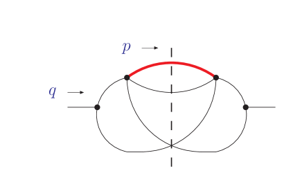
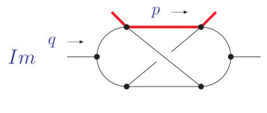
Figure 1: Examples of Feynman integrals from $e^{+}e^{-}$-annihilation (left) and deep-inelastic scattering (right). All propagators have unit power.

3.1 $e^{+}e^{-}$-annihilation

The example which stems from single hadron inclusive $e^{+}e^{-}$-annihilation is a phase space integral for a decay process $1\to 4$ in one-particle inclusive kinematics, see Fig. 1 on the left. The scalar diagram describes the decay of a particle with initial momentum $q$ according to $q\to p_{1}+p_{2}+p_{3}+p$ and the dashed vertical line denotes the final-state cut for the production of particles. Our example is the master integral ${\mbox{R}}_{2}(N)$ from the so-called real-real-emission and it depends on the dimensionless variable $x_{E}$ which is the scaled momentum fraction

$$x_{E}={2p\cdot q\over q\cdot q}\,,\quad\quad\quad 0\leq x_{E}\leq 1\,.$$ (11)

The solution of the integration-by-parts identities leads to a difference equation of second order [9], which reflects the underlying symmetries of the Feynman diagram. We find

$$(N+1-2\*\epsilon)\*(N+2-6\*\epsilon)\*{\mbox{R}}_{2}(N)-(N-1)\*(N-4\*\epsilon)\*{\mbox{R}}_{2}(N-2)\,=\,$$ (12)

$$\qquad\qquad\qquad\qquad 2\*{{(1-\epsilon)\*(1-3\*\epsilon)\*(2-3\*\epsilon)\*(2\*N+1-6\*\epsilon)}\over{(N-3\*\epsilon)\*(N+1-3\*\epsilon)}}\,\*{\mbox{R}}_{1}(N-2)\>\>,$$

where ${\mbox{R}}_{1}$ denotes the inhomogeneous part. For a complete solution, we also have to provide the initial conditions ${\mbox{R}}_{2}(0)$ and ${\mbox{R}}_{2}(1)$. The explicit expressions are rather lengthy, in particular the higher powers in the Laurent series in $\epsilon$ and we refer the reader to [9] for details.

We have provided Sigma with the difference equation (12) and the expression for ${\mbox{R}}_{1}$ in terms of harmonic sums. Subsequently Sigma was able to solve for ${\mbox{R}}_{2}(N)$ and we have found complete agreement with the published result after insertion of the initial conditions ${\mbox{R}}_{2}(0)$ and ${\mbox{R}}_{2}(1)$.

3.2 Deep-inelastic scattering

During the computation of the three-loop QCD corrections to the DIS structure functions $F_{2}$ and $F_{L}$ we have encountered the Feynman integral shown in Fig. 1 (right). The scalar diagram in the DIS case has external momenta $p$ and $q$ and is of the non-planar topology ${\mbox{NO}}_{22}$ with unit powers of the propagators. Due to the framework of the operator product expansion and the optical theorem applied in DIS, we are specifically interested in the imaginary part of ${\mbox{NO}}_{22}$. In momentum space it depends on the scaling variable $x_{B}$,

$$x_{B}={-q\cdot q\over 2p\cdot q}\,,\quad\quad\quad 0\leq x_{B}\leq 1\,.$$ (13)

In Mellin space the associated difference equation is of third order and very difficult [8]. It has been obtained by means of a systematic solution of the integration-by-parts identities and is given by

$$-{\mbox{NO}}_{22}(N)\*N\*(N-2)\*(3\*N-5)\*(N^{2}-1)$$

$$+{\mbox{NO}}_{22}(N-1)\*N\*(3\*N^{4}-20\*N^{3}+45\*N^{2}-40\*N+12)$$

$$+{\mbox{NO}}_{22}(N-2)\*N\*(3\*N^{4}-17\*N^{3}+35\*N^{2}-31\*N+10)$$

$$-{\mbox{NO}}_{22}(N-3)\*(N-1)\*(N-2)^{2}\*(3\*N-2)\*(N-3)\,=\,2\*{\mbox{X}}(N)\,,$$ (14)

where we have put $\epsilon=0$, since the integral ${\mbox{NO}}_{22}$ does not contain any divergences. It is completely finite and to the accuracy needed in the three-loop calculation [8] positive powers in $\epsilon$ were not necessary.

For the solution of Eq. (3.2), we have to provide the inhomogeneous part X (which is also finite),

$${\mbox{X}}(N) = 32\*{\zeta_{3}}+56\*{S_{-3}(N-3)\over N-3}-8\*{S_{-3}(N-2)\over N-2}+20\*S_{-3}(N)+108\*{S_{-2}(N-3)\over N-3}+56\*{S_{-2}(N-3)\over(N-3)^{2}}$$

$$-36\*{S_{-2}(N-2)\over N-2}-8\*{S_{-2}(N-2)\over(N-2)^{2}}+12\*S_{-2}(N)+12\*{S_{2}(N-2)\over N-2}+16\*{S_{2}(N-2)\over(N-2)^{2}}$$

$$-12\*{S_{2}(N-1)\over N-1}+8\*{S_{2}(N-1)\over(N-1)^{2}}-12\*S_{2}(N)-16\*{S_{3}(N-2)\over N-2}-8\*{S_{3}(N-1)\over N-1}-4\*S_{3}(N)$$

$$+84\*{{\zeta_{3}}\over N-3}+24\*{1\over N-2}-4\*{{\zeta_{3}}\over N-2}+92\*{1\over(N-2)^{2}}+56\*{1\over(N-2)^{3}}-48\*{1\over N-1}+4\*{{\zeta_{3}}\over N-1}$$

$$-100\*{1\over(N-1)^{2}}-36\*{1\over(N-1)^{3}}+48\*{1\over N}+76\*{1\over N^{2}}+20\*{1\over N^{3}}+(-1)^{N}\*\biggl{(}-24\*{\zeta_{3}}-72\*N\*{\zeta_{3}}$$

$$-56\*{S_{-3}(N-3)\over N-3}-24\*{S_{-3}(N-2)\over N-2}+8\*{S_{-3}(N-1)\over N-1}-16\*S_{-3}(N)-48\*S_{-3}(N)\*N$$

$$-108\*{S_{-2}(N-3)\over N-3}-56\*{S_{-2}(N-3)\over(N-3)^{2}}-24\*{S_{-2}(N-2)\over N-2}+8\*{S_{-2}(N-2)\over(N-2)^{2}}+12\*{S_{-2}(N-1)\over N-1}$$

$$-8\*{S_{-2}(N-1)\over(N-1)^{2}}-16\*S_{-2}(N)-48\*S_{-2}(N)\*N-84\*{{\zeta_{3}}\over N-3}-24\*{1\over N-2}-36\*{{\zeta_{3}}\over N-2}$$

$$-92\*{1\over(N-2)^{2}}-56\*{1\over(N-2)^{3}}+12\*{{\zeta_{3}}\over N-1}+12\*{1\over(N-1)^{2}}+20\*{1\over(N-1)^{3}}-12\*{1\over N^{2}}-20\*{1\over N^{3}}\biggr{)}\,,$$

along with the initial conditions ${\mbox{NO}}_{22}(0)$, ${\mbox{NO}}_{22}(1)$ and ${\mbox{NO}}_{22}(2)$. Here, $\zeta_{i}$ denotes the Riemann $\zeta$-function at value $i$.

We have again used Sigma for solving the difference equation (3.2), given the expression for X from Eq. (3.2) and Sigma has provided us with the correct analytical answer for ${\mbox{NO}}_{22}$ once also the initial conditions ${\mbox{NO}}_{22}(0)$, ${\mbox{NO}}_{22}(1)$ and ${\mbox{NO}}_{22}(2)$ had been supplied. The solution is given by the following very compact expression,

$$\displaystyle{\mbox{NO}}_{22}(N) = \frac{2\left(6{\zeta_{3}}+(-1)^{N}\left(6{\zeta_{3}}-5N^{2}{\zeta_{5}}\right)\right)}{N^{2}(N+1)}$$

$$-\frac{8\left(1+(-1)^{N}\right)S_{-5}(N)}{N+1}-\frac{4\left(1+(-1)^{N}\right)S_{5}(N)}{N+1}+S_{2}(N)\left(\frac{4S_{3}(N)}{N+1}-\frac{4{\zeta_{3}}}{N+1}\right)$$

$$+S_{-3}(N)\left(\frac{8\left(1+(-1)^{N}\right)}{N^{2}(N+1)}-\frac{4\left(2+(-1)^{N}\right)S_{-2}(N)}{N+1}-\frac{4S_{2}(N)}{N+1}\right)$$

$$+S_{-2}(N)\left(\frac{-12{\zeta_{3}}N^{3}+(-1)^{N}\left(8-8N^{3}{\zeta_{3}}\right)+8}{N^{3}(N+1)}-\frac{\left(4+8(-1)^{N}\right)S_{3}(N)}{N+1}\right)$$

$$+\frac{8S_{-3,-2}(N)}{N+1}+\frac{\left(4-4(-1)^{N}\right)S_{-3,2}(N)}{N+1}+\frac{\left(4+12(-1)^{N}\right)S_{-2,3}(N)}{N+1}-\frac{8S_{2,3}(N)}{N+1}\,,$$

where we have eliminated a number of nested sums in favor of products of harmonic sums through their product algebra, leaving only four independent sums of depth two.

4 Summary

In these proceedings, we have presented a short introduction to the problem of calculating Feynman integrals at multiple loops. For single-scale problems we have sketched how to formulate the problem in Mellin space, how to obtain algebraic reductions for the loop integrals and, finally, how these reductions lead to difference equations in Mellin space. While the underlying physics problem usually places certain restrictions on the difference equations, which allow for their solutions to be expressed in terms of harmonic sums, and hence to be constructed with a corresponding ansatz, it is advantageous to reconsider the problem in a more general mathematical framework.

We have reported on progress in this direction by exploiting algebraic properties of difference fields, the so-called $\Pi\Sigma^{*}$-fields. The algorithmic construction of analytical solutions to the recursion relations for Feynman integrals over difference fields as, for instance, implemented in the Mathematica package Sigma provides great calculational advantages. To that end, we have tested the package Sigma on two examples of Feynman integrals which had appeared in recent perturbative higher-order QCD computations for $e^{+}e^{-}$-annihilation and deep-inelastic scattering. With the improved mathematical machinery both examples have been re-evaluated with the package Sigma and we have found agreement.

In the future more generalizations or extensions are conceivable. From the need to consider physics problems and Feynman integrals depending on multiple scales one arrives at generalized sums [30], which in turn are connected to multiple and harmonic polylogarithms [31, 32]. A related problem is the expansion of (generalized) hypergeometric functions around integer or rational values in a small parameter  These problems lead to recursion relations similar to Eqs. (4) or (5) although with functional or parametric dependences on more variables. Some algorithms and implementations exist [33, 34, 35, 36] and it will be interesting to pursue this line of research further within the framework of $\Pi\Sigma^{*}$-fields.

Acknowledgements:  This research draws upon (partly still unpublished) results obtained by S.M. together with A. Mitov, A. Vogt and J. Vermaseren and S.M. would like to thank them for very pleasant collaborations. The work of S.M. has been supported by the Helmholtz Gemeinschaft under contract VH-NG-105 and in part by the Deutsche Forschungsgemeinschaft in Sonderforschungsbereich/Transregio 9. C.S. was supported by the SFB grant F1305 of the Austrian Science Foundation FWF.

References

- [1] V.A. Smirnov, Springer Tracts Mod. Phys. 211 (2004) 1.
- [2] D.I. Kazakov and A.V. Kotikov, Nucl. Phys. B307 (1988) 721.
- [3] S. Moch and J.A.M. Vermaseren, Nucl. Phys. B573 (2000) 853, hep-ph/9912355.
- [4] A. Mitov, Phys. Lett. B643 (2006) 366, hep-ph/0511340.
- [5] S. Moch, Nucl. Instrum. Meth. A559 (2006) 285, math-ph/0509058.
- [6] S. Moch, J.A.M. Vermaseren and A. Vogt, Nucl. Phys. B688 (2004) 101, hep-ph/0403192.
- [7] A. Vogt, S. Moch and J.A.M. Vermaseren, Nucl. Phys. B691 (2004) 129, hep-ph/0404111.
- [8] J.A.M. Vermaseren, A. Vogt and S. Moch, Nucl. Phys. B724 (2005) 3, hep-ph/0504242.
- [9] A. Mitov and S. Moch, Nucl. Phys. B751 (2006) 18, hep-ph/0604160.
- [10] D. Zeilberger, J. Symbolic Comput. 11 (1991) 195.
- [11] S.K. I. Bierenbaum, J. Blümlein and C. Schneider, (2007), arXiv:0707.4659 [math-ph].
- [12] J.A.M. Vermaseren, (2000), math-ph/0010025.
- [13] J.A.M. Vermaseren, Int. J. Mod. Phys. A14 (1999) 2037, hep-ph/9806280.
- [14] C. Schneider, Sém. Lothar. Combin. 56 (2007) 1, Article B56b.
- [15] M. Karr, J. ACM 28 (1981) 305.
- [16] C. Schneider, Ann. Comb. 9 (2005) 75.
- [17] C. Schneider, J. Differ. Equations Appl. 11 (2005) 799.
- [18] M. Bronstein, J. Symbolic Comput. 29 (2000) 841.
- [19] C. Schneider, Proc. SYNASC’04, edited by D.P. et al., pp. 269–282, Mirton Publishing, 2004.
- [20] C. Schneider, Appl. Algebra Engrg. Comm. Comput. 16 (2005) 1.
- [21] S. Abramov and M. Petkovšek, Proc. ISSAC’94, edited by J. von zur Gathen, pp. 169–174, ACM Press, 1994.
- [22] P. Hendriks and M. Singer, J. Symbolic Comput. 27 (1999) 239.
- [23] C. Schneider, RISC-Linz, J. Kepler University preprint 01-17 (2001), PhD Thesis.
- [24] M. Petkovšek, J. Symbolic Comput. 14 (1992) 243.
- [25] J. Blümlein, Comput. Phys. Commun. 159 (2004) 19, hep-ph/0311046.
- [26] C. Schneider, Proc. ISSAC’05, edited by M. Kauers, pp. 285–292, ACM, 2005.
- [27] M. Kauers and C. Schneider, Proc. ISSAC’07, edited by C.W. Brown, pp. 219–226, 2007.
- [28] M. Kauers and C. Schneider, Discrete Math. 306 (2006) 2021.
- [29] M. Kauers and C. Schneider, Proc. ISSAC’06., edited by J. Dumas, pp. 177–183, ACM Press, 2006.
- [30] S. Moch, P. Uwer and S. Weinzierl, J. Math. Phys. 43 (2002) 3363, hep-ph/0110083.
- [31] A.B. Goncharov, Math. Res. Lett. 5 (1998) 497, (available at http://www.math.uiuc.edu/K-theory/0297).
- [32] E. Remiddi and J.A.M. Vermaseren, Int. J. Mod. Phys. A15 (2000) 725, hep-ph/9905237.
- [33] S. Weinzierl, Comput. Phys. Commun. 145 (2002) 357, math-ph/0201011.
- [34] S. Weinzierl, J. Math. Phys. 45 (2004) 2656, hep-ph/0402131.
- [35] S. Moch and P. Uwer, Comput. Phys. Commun. 174 (2006) 759, math-ph/0508008.
- [36] T. Huber and D. Maitre, (2007), arXiv:0708.2443 [hep-ph].