Two ferromagnetic phases in spin-Fermion systems

Abstract

We consider spin-Fermion systems which obtain their magnetic properties from a system of localized magnetic moments being coupled to conducting electrons. The dynamical degrees of freedom are spin-$s$ operators of localized spins and spin-$1/2$ Fermi operators of itinerant electrons. We develop modified spin-wave theory and obtain that system has two ferromagnetic phases. At the characteristic temperature $T^{*}$, the magnetization of itinerant electrons becomes zero, and high temperature ferromagnetic phase ($T^{*}<T<T_{C}$) is a phase where only localized electrons give contribution to the magnetization of the system. An anomalous increasing of magnetization below $T^{*}$ is obtained in good agrement with experimental measurements of the ferromagnetic phase of $UGe_{2}$.

This Brief Report is inspired from the experimental measurements of the ferromagnetic phase of $UGe_{2}$ which reveal the presence of an additional phase line that lies entirely within the ferromagnetic phase. The characteristic temperature of this transition $T^{*}$, which is below the Curie temperature $T_{C}$, decreases with pressure and disappears at a pressure close to the pressure at which new phase of coexistence of superconductivity and ferromagnetism emerges2fmp1 ; 2fmp2 ; 2fmp3 .Strong anomaly in resistivity is observed at $T^{*}$ 2fmp4 . The additional phase transition demonstrates itself and through the change in the $T$ dependence of the ordered ferromagnetic moment2fmp2 ; 2fmp5 ; 2fmp6 ; 2fmp7 . The magnetization shows an anomalous enhancement below $T^{*}$. An anomaly is found in the heat capacity at the characteristic temperature $T^{*}$ 2fmp8 . Theoretically, it was assumed that the interplay of charge-density wave and spin-density wave fluctuations is the origin of anomalous properties2fmp8a . Alternatively, it was proposed that the unusual phase diagram is result of novel tuning of the Fermi surface topology by the magnetization2fmp8b .

Our objective is spin-Fermion systems, which obtain their magnetic properties from a system of localized magnetic moments and itinerant electrons. It is obtained that the true magnons in these systems, which are the transversal fluctuations corresponding to the total magnetization, are complicate mixture of the transversal fluctuations of the spins of localized and itinerant electrons. The magnons interact with different spins in a different way, and magnons’ fluctuations suppress the ordered moments of the localized and itinerant electrons at different temperatures. As a result, the ferromagnetic phase is divided onto two phases: low temperature phase $0<T<T^{*}$, where all electrons contribute the ordered ferromagnetic moment, and high temperature phase $T^{*}<T<T_{C}$, where only localized spins form magnetic moment. To describe the two phases, a modified spin-wave theory is developed. We have reproduced theoretically the anomalous temperature dependence of the ordered moment, known from the experiments with $UGe_{2}$ 2fmp2 ; 2fmp5 ; 2fmp6 ; 2fmp7 .

The spin-fermion model is known as $s-d$ (or $s-f$). The model appears in the literature also as the ferromagnetic Kondo Lattice model (FKLM) or the double exchange model (DEM). The exact results for the spin-Fermion model are reported in 2fmp8c .

The dynamical degrees of freedom are spin-$s$ operators of localized spins and spin-$1/2$ Fermi operators of itinerant electrons. We consider a theory with Hamiltonian

$$h = H-\mu N=-t\sum\limits_{\langle ij\rangle}{\left({c_{i\sigma}^{+}c_{j\sigma}+h.c.}\right)}-\mu\sum\limits_{i}{n_{i}}$$ (1)

$$- J^{l}\sum\limits_{\langle ij\rangle}{{\bf S}_{i}\cdot{\bf S}_{j}}-J\sum\limits_{i}{{\bf S}_{i}}\cdot{\bf s}_{i}$$

where $s^{\nu}_{i}=\frac{1}{2}\sum\limits_{\sigma\sigma^{\prime}}c^{+}_{i\sigma}\tau^{\nu}_{\sigma\sigma^{\prime}}c^{\phantom{+}}_{i\sigma^{\prime}}$, with the Pauli matrices $(\tau^{x},\tau^{y},\tau^{z})$, is the spin of the conduction electrons, ${\bf S}_{i}$ is the spin of the localized electrons, $\mu$ is the chemical potential, and $n_{i}=c^{+}_{i\sigma}c_{i\sigma}$. The sums are over all sites of a three-dimensional cubic lattice, and $\langle i,j\rangle$ denotes the sum over the nearest neighbors. The Heisenberg term $(J^{l}>0)$ describes ferromagnetic Heisenberg exchange between nearest-neighbors localized electrons. The term which describes the spin-Fermion interaction $(J>0)$ is known as a Kondo interaction $(J=J_{K})$ in the ferromagnetic Kondo model or as a Hund’s term in the double exchange model ($J=J_{H}$ and $J^{l}<0$).

We represent the Fermi operators in terms of the Schwinger bosons ($\varphi_{i,\sigma},\varphi_{i,\sigma}^{+}$) and slave Fermions ($h_{i},h_{i}^{+},d_{i},d_{i}^{+}$). The Bose fields are doublets $(\sigma=1,2)$ without charge, while Fermions are spinless with charges 1 ($d_{i}$) and -1 ($h_{i}$).

$$c_{i\uparrow}=h_{i}^{+}\varphi_{i1}+\varphi_{i2}^{+}d_{i},\qquad c_{i\downarrow}=h_{i}^{+}\varphi_{i2}-\varphi_{i1}^{+}d_{i},$$

$$n_{i}=1-h^{+}_{i}h_{i}+d^{+}_{i}d_{i},\quad s^{\nu}_{i}=\frac{1}{2}\sum\limits_{\sigma\sigma^{\prime}}\varphi^{+}_{i\sigma}{\tau}^{\nu}_{\sigma\sigma^{\prime}}\varphi_{i\sigma^{\prime}},$$

$$\varphi_{i1}^{+}\varphi_{i1}+\varphi_{i2}^{+}\varphi_{i2}+d_{i}^{+}d_{i}+h_{i}^{+}h_{i}=1$$ (2)

Next, we make a change of variables, introducing Bose doublets $\zeta_{i\sigma}$ and $\zeta^{+}_{i\sigma}\,$2fmp9

$$\zeta_{i\sigma} = \varphi_{i\sigma}\left(1-h^{+}_{i}h_{i}-d^{+}_{i}d_{i}\right)^{-\frac{1}{2}},$$

$$\zeta^{+}_{i\sigma} = \varphi^{+}_{i\sigma}\left(1-h^{+}_{i}h_{i}-d^{+}_{i}d_{i}\right)^{-\frac{1}{2}},$$ (3)

where the new fields satisfy the constraint $\zeta^{+}_{i\sigma}\zeta_{i\sigma}\,=\,1$. In terms of the new fields the spin vectors of the itinerant electrons have the form

$$s^{\nu}_{i}=\frac{1}{2}\sum\limits_{\sigma\sigma^{\prime}}\zeta^{+}_{i\sigma}{\tau}^{\nu}_{\sigma\sigma^{\prime}}\zeta_{i\sigma^{\prime}}\left[1-h^{+}_{i}h_{i}-d^{+}_{i}d_{i}\right]$$ (4)

When, in the ground state, the lattice site is empty, the operator identity $h^{+}_{i}h_{i}=1$ is true. When the lattice site is doubly occupied, $d^{+}_{i}d_{i}=1$. Hence, when the lattice site is empty or doubly occupied the spin on this site is zero. When the lattice site is neither empty nor doubly occupied ($h^{+}_{i}h_{i}=d^{+}_{i}d_{i}=0$), the spin equals $\,\,{\bf s}_{i}=1/2{\bf n}_{i},\,\,$ where the unit vector $\,\,n^{\nu}_{i}=\sum\limits_{\sigma\sigma^{\prime}}\zeta^{+}_{i\sigma}{\tau}^{\nu}_{\sigma\sigma^{\prime}}\zeta_{i\sigma^{\prime}}\,\,\,({\bf n}_{i}^{2}=1)\,\,$ identifies the local orientation of the spin of the itinerant electron. Let us average the spin of electrons in the subspace of the Fermions $(d^{+}_{i},\,d_{i})$ and $(h^{+}_{i},\,h_{i})$ (to integrate the Fermions out in the path integral approach) and introduce the notation

$$m=\frac{1}{2}\left(1-<h^{+}_{i}h_{i}>-<d^{+}_{i}d_{i}>\right).$$ (5)

One obtains ${\bf s}_{i}=m{\bf n}_{i}$ where ${\bf s}_{i}^{2}=m^{2}$. Hence, the amplitude of the spin vector $m$ is an effective spin of the itinerant electrons accounting for the fact that some sites, in the ground state, are doubly occupied or empty.

It is more convenient to use the rescaled Bose fields

$$\xi_{i\sigma}=\sqrt{2m}\,\zeta_{i\sigma},\qquad\qquad\xi^{+}_{i\sigma}=\sqrt{2m}\,\zeta^{+}_{i\sigma}$$ (6)

which satisfy the constraint $\xi^{+}_{i\sigma}\xi_{i\sigma}=2m$. Let us introduce the vector,

$$M^{\nu}_{i}=\frac{1}{2}\sum\limits_{\sigma\sigma^{\prime}}\xi^{+}_{i\sigma}{\tau}^{\nu}_{\sigma\sigma^{\prime}}\xi_{i\sigma^{\prime}}\quad{\bf M}_{i}^{2}=m^{2}.$$ (7)

Then, the spin-vector of itinerant electrons can be written in the form

$${\bf s}_{i}=\frac{1}{2m}{\bf M}_{i}\left(1-h^{+}_{i}\,h_{i}\,-\,d^{+}_{i}\,d_{i}\right)$$ (8)

The contribution of itinerant electrons to the total magnetization is $<{\bf s}^{z}_{i}>$. Accounting for the definition of $m$ (see Eq.5), one obtains $<{\bf s}^{z}_{i}>=<{\bf M}^{z}_{i}>$.

The Hamiltonian is quadratic with respect to the Fermions $d_{i},d^{+}_{i}$ and $h_{i},h^{+}_{i}$, and one can average in the subspace of these Fermions (to integrate them out in the path integral approach). As a result, we obtain an effective theory of two spin-vectors ${\bf S}_{i}$ and ${\bf M}_{i}$ with Hamiltonian

$$h_{eff}=-J^{l}\sum\limits_{\langle ij\rangle}{{\bf S}_{i}\cdot{\bf S}_{j}}-J^{it}\sum\limits_{\langle ij\rangle}{{\bf M}_{i}\cdot{\bf M}_{j}}-J\sum\limits_{i}{{\bf S}_{i}}\cdot{\bf M}_{i}$$ (9)

The first term is the term which describes the exchange of localized spins in the Hamiltonian Eq.(1). The second term is obtained integrating out the Fermions. It is calculated in the one loop approximation and in the limit when the frequency and the wave vector are small. For the effective exchange constant $J^{it}$, at zero temperature, we obtained

$$J^{it}=$$

$$\frac{t}{6m^{2}}\frac{1}{N}\sum\limits_{k}\left(\sum\limits_{\nu=1}^{3}\cos k_{\nu}\right)\left[1-\theta(-\varepsilon^{h}_{k})+\theta(-\varepsilon^{d}_{k})\right]$$

$$- \frac{2t^{2}}{3m^{2}sJ}\frac{1}{N}\sum\limits_{k}\left(\sum\limits_{\nu=1}^{3}\sin^{2}k_{\nu}\right)\left[1-\theta(-\varepsilon^{h}_{k})-\theta(-\varepsilon^{d}_{k})\right]$$

where $N$ is the number of lattice’s sites, $\varepsilon^{h}_{k}$ and $\varepsilon^{d}_{k}$ are Fermions’ dispersions,

$$\varepsilon^{h}_{k} = 2t(\cos k_{x}+\cos k_{y}+\cos k_{z})+stJ/2+\mu$$ (11)

$$\varepsilon^{d}_{k} = -2t(\cos k_{x}+\cos k_{y}+\cos k_{z})+stJ/2-\mu,$$

and wave vector $k$ runs over the first Brillouin zone of a cubic lattice. The third term in Eq.(9) is obtained from the last term in the Hamiltonian Eq.(1) using the representation Eq.(8) for the spin of itinerant electrons and Eq.(5).

We are going to study the ferromagnetic phase of the two-spin system Eq.(9) with $J^{l}>0,\,\,J^{it}>0$, and $J>0$. To proceed we use the Holstein-Primakoff representation of the spin vectors ${\bf S}_{j}(a^{+}_{j},a_{j})$ and ${\bf M}_{j}(b^{+}_{j},\,b_{j})$, where $a^{+}_{j},\,a_{j}$ and $b^{+}_{j},\,b_{j}$ are Bose fields. In terms of these fields and keeping only the quadratic terms, the effective Hamiltonian Eq.(9) adopts the form

$$h_{eff} = s\,J^{l}\sum\limits_{\langle ij\rangle}(a_{i}^{+}a_{i}+a_{j}^{+}a_{j}-a_{j}^{+}a_{i}-a_{i}^{+}a_{j})$$

$$+ m\,J^{it}\sum\limits_{\langle ij\rangle}(b^{+}_{i}b_{i}+b^{+}_{j}b_{j}-b^{+}_{j}b_{i}-b^{+}_{i}b_{j})$$

$$- J\sum\limits_{i}(\sqrt{sm}\,[a_{i}^{+}b_{i}+b_{i}^{+}a_{i}]-sb_{i}^{+}b_{i}-ma_{i}^{+}a_{i})$$

In momentum space representation, the Hamiltonian reads

$$h_{eff}=\sum\limits_{k}\left(\varepsilon^{a}_{k}\,a_{k}^{+}a_{k}\,+\,\varepsilon^{b}_{k}\,b_{k}^{+}b_{k}\,-\,\gamma\,(a_{k}^{+}b_{k}+b_{k}^{+}a_{k})\,\right),$$ (13)

where the dispersions are given by equalities,

$$\varepsilon^{a}_{k}\,=\,2sJ^{l}\,\varepsilon_{k}\,+\,m\,J,\qquad\varepsilon^{b}_{k}\,=\,2mJ^{it}\,\varepsilon_{k}\,+\,s\,J,$$ (14)

$\varepsilon_{k}=3-\cos k_{x}-\cos k_{y}-\cos k_{z}$, and $\gamma\,=\,J\,\sqrt{s\,m}$.

To diagonalize the Hamiltonian, one introduces Bose fields $\alpha_{k},\,\alpha_{k}^{+},\,\beta_{k},\,\beta_{k}^{+}$,

$$a_{k}\,=\cos\theta_{k}\,\alpha_{k}\,+\,\sin\theta_{k}\,\beta_{k},\quad b_{k}\,=\,-\sin\theta_{k}\,\alpha_{k}\,+\,\cos\theta_{k}\,\beta_{k}$$ (15)

with coefficients of transformation,

$$\cos\theta_{k}\,=\,\sqrt{\frac{1}{2}\,\left(1+\frac{\varepsilon^{a}_{k}-\varepsilon^{b}_{k}}{\sqrt{(\varepsilon^{a}_{k}-\varepsilon^{b}_{k})^{2}+4\gamma^{2}}}\right)},$$ (16)

and $\sin\theta_{k}=(1-\cos^{2}\theta_{k})^{1/2}$. The transformed Hamiltonian

$$h_{eff}=\sum\limits_{k}\left(E^{\alpha}_{k}\,\alpha_{k}^{+}\alpha_{k}\,+\,E^{\beta}_{k}\,\beta_{k}^{+}\beta_{k}\right),$$ (17)

where

$$E^{\pm}_{k}\,=\,\frac{1}{2}\,\left[\varepsilon^{a}_{k}+\varepsilon^{b}_{k}\,\pm\,\sqrt{(\varepsilon^{a}_{k}-\varepsilon^{b}_{k})^{2}+4\gamma^{2}}\right]$$ (18)

, and $E^{\alpha}_{k}=E^{+}_{k},\,\,E^{\beta}_{k}=E^{-}_{k}$. With positive exchange constants $J^{l}>0,\,J^{it}>0$, and $J>0$, the bose fields’ dispersions are positive $\varepsilon^{a}_{k}>0,\,\,\varepsilon^{b}_{k}>0$ for all wave vectors $k$. As a result, $E^{\alpha}_{k}>0$ and $E^{\beta}_{k}\geq 0$ with $E^{\beta}_{0}=0$. Near the zero wave vector, $E^{\beta}_{k}\approx\rho k^{2}$ where the spin-stiffness constant is $\rho=(s^{2}J^{l}\,+\,m^{2}J^{it})/(s+m)$. Hence, $\beta_{k}$ is the long-range (magnon) excitation in the two-spin effective theory, while $\alpha_{k}$ is a gapped excitation with gap $E^{\alpha}_{0}\,=\,(s+m)J$.

The dimensionless magnetization per lattice site of the system $M$ is a sum of the magnetization of the localized electrons $M^{l}\,=\,<S^{z}_{i}>$ and the magnetization of the itinerant electrons $M^{it}\,=\,<s^{z}_{i}>\,=\,<M^{z}_{i}>$,  $(M\,=\,M^{l}\,+\,M^{it})$. By means of the Holstein-Primakoff representation the magnetizations adopts the form $M^{l}=s-1/N\sum\limits_{k}<a^{+}_{k}a_{k}>,\,\,M^{it}=m-1/N\sum\limits_{k}<b^{+}_{k}b_{k}>$. Finally, by means of the transformation Eq.(15) one can rewrite $M^{l}$ and $M^{it}$ in terms of the Bose functions of the excitations $\alpha_{k}$-$n^{\alpha}_{k}$ and $\beta_{k}$-$n^{\beta}_{k}$

$$M^{l}\,=\,s-\frac{1}{N}\sum\limits_{k}\left[\cos^{2}\theta_{k}\,n^{\alpha}_{k}\,+\,\sin^{2}\theta_{k}\,n^{\beta}_{k}\right],$$ (19)

$$M^{it}\,=\,m-\frac{1}{N}\sum\limits_{k}\left[\sin^{2}\theta_{k}\,n^{\alpha}_{k}\,+\,\cos^{2}\theta_{k}\,n^{\beta}_{k}\right].$$

The magnetization of the system is

$$M\,=\,s\,+\,m-\frac{1}{N}\sum\limits_{k}\left[n^{\alpha}_{k}\,+\,n^{\beta}_{k}\right].$$ (20)

The magnon excitation $\beta_{k}$ in the effective theory Eq.(9) is a complicate mixture of the transversal fluctuations of the spins of localized and itinerant electrons Eq.(15). As a result, the magnons’ fluctuations suppress in a different way the magnetic order of these electrons. Quantitatively, this depends on the coefficients $\cos\theta_{k}$ and $\sin\theta_{k}$ in Eqs.(19). If the spin-Fermion interaction is very strong, $J\gg J^{it}$ and $J\gg J^{l}$, one can calculate the coefficients approximately using approximate expressions for dispersions Eqs. (14): $\varepsilon^{a}_{k}\approx mJ,and\varepsilon^{a}_{k}\approx sJ$. As a result, one obtains $\cos^{2}\theta_{k}\approx m/(m+s)$. For large $J$, the gap of the $\alpha$ excitation is very big, $E^{\alpha}_{0}\,=\,(s+m)J$, and one can drop this excitation in the calculations. Then, the approximate expressions for magnetization satisfy $M^{l}/s\,=M^{it}/m$, which means that the strong spin-Fermion interaction aligns the magnetic orders of the itinerant and localized electrons so strong that they become zero at one and just the same temperature. The result is different if the spin-Fermion interaction is relatively small. The magnetization depends on the dimensionless temperature $T/J$ and dimensionless parameters $s,\,m,\,J^{l}/J$ and $J^{it}/J$. We consider a theory with spin of the localized electrons $s=1$ and calculate the parameters of the effective theory Eq.(9) in one Fermion-loop approximation for density of Fermions $n=0.4$ and microscopic parameter $J/t=12.4$. The result is $m=0.2$ and $J^{it}/J=0.1$. Finally, we set $J^{l}/J=0.5$. For these effective parameters, the functions $M(T/J)$, $M^{l}(T/J)$, and $M^{it}(T/J)$ are depicted in Fig.1 The green line is the magnetization of the localized electrons, the red line is the magnetization of the itinerant electrons, and the blue line is the total magnetization. The figure shows that the magnetic order of itinerant electrons (red line) is suppressed first, at temperature $T^{*}/J=0.5603$. Once suppressed, the magnetic order cannot be restored at temperatures above $T^{*}$ because of the increasing effect of magnon fluctuations. Hence, the magnetization of the itinerant electrons should be zero above $T^{*}$. As is evident from Fig.1, this is not the result within customary spin-wave theory.

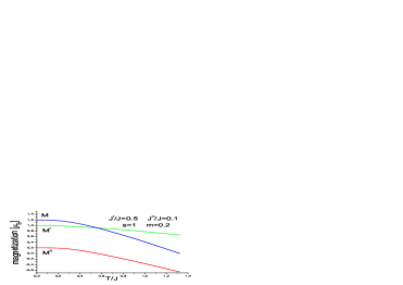
Figure 1: (color online) Temperature dependence of the ferromagnetic moments: $M$ (blue line)-the magnetization of the system, $M^{l}$ (green line)-contribution of the localized electrons, $M^{it}$ (red line)-contribution of the itinerant electrons for parameters $s=1,\,m=0.2,\,J^{l}/J=0.5$ and $J^{it}/J=0.1$:  spin-wave theory

To solve the problem, we use the idea on description of paramagnetic phase of two-dimensional ferromagnets ($T>0$) by means of modified spin-wave theory 2fmp10 ; 2fmp11 . In the simplest version, the spin-wave theory is modified by introducing a parameter which enforces the magnetization of the system to be equal to zero in paramagnetic phase.

In the present case, we have two-spin system and we introduce two parameters $\lambda^{l}$ and $\lambda^{it}$ to enforce the magnetic moments both of the localized and the itinerant electrons to be equal to zero in paramagnetic phase. To this end, we add two new terms to the effective Hamiltonian Eq.(Two ferromagnetic phases in spin-Fermion systems),

$$\hat{h}_{eff}\,=\,h_{eff}\,-\,\sum\limits_{i}\left[\lambda^{l}S^{z}_{i}\,+\,\lambda^{it}M_{i}^{z}\right].$$ (21)

In momentum space, the Hamiltonian adopts the form Eq.(13) with new dispersions $\hat{\varepsilon}^{a}_{k}=\varepsilon^{a}_{k}+\lambda^{l}$ and $\hat{\varepsilon}^{b}_{k}=\varepsilon^{b}_{k}+\lambda^{it}$, where the old dispersions are given by equalities (14). We utilize the same transformation Eq.(15) with coefficients $\cos\hat{\theta}_{k}$ and $\sin\hat{\theta}_{k}$ which depend on the new dispersions in the same way as the old ones depend on the old dispersions Eq.(16). In terms of the $\alpha_{k}$ and $\beta_{k}$ bosons, the Hamiltonian $\hat{h}_{eff}$ adopts the form Eq.(17) with dispersions $\hat{E}^{\alpha}_{k}$ and $\hat{E}^{\beta}_{k}$, which can be written in the form Eq.(18) replacing $\varepsilon^{a}_{k}$ and $\varepsilon^{b}_{k}$ with $\hat{\varepsilon}^{a}_{k}$ and $\hat{\varepsilon}^{b}_{k}$.

We have to do some assumptions for parameters $\lambda^{l}$ and $\lambda^{it}$ to ensure correct definition of the two-boson theory. For that purpose, it is convenient to represent the parameters $\lambda^{l}$ and $\lambda^{it}$ in the form $\lambda^{l}\,=\,mJ\mu^{l}\,-\,mJ,and\lambda^{it}\,=\,sJ\mu^{it}\,-\,sJ$. In terms of the parameters $\mu^{l}$ and $\mu^{it}$, the dispersion reads $\hat{\varepsilon}^{a}_{k}=2sJ^{l}\,\varepsilon_{k}+mJ\mu^{l},\,\,\,\hat{\varepsilon}^{b}_{k}=2mJ^{it}\varepsilon_{k}+sJ\mu^{it}$ The conventional spin-wave theory is reproduced when $\mu^{l}=\mu^{it}=1$($\lambda^{l}=\lambda^{it}=0$). We assume $\mu^{l}$ and $\mu^{it}$ to be positive ($\mu^{l}>0,\,\mu^{it}>0$). Then, $\hat{\varepsilon}^{a}_{k}>0$, $\hat{\varepsilon}^{b}_{k}>0$, and $\hat{E}^{\alpha}_{k}>0$ for all values of the wave-vector $k$. To explore the dispersion $\hat{E}^{\beta}_{k}=\frac{1}{2}\left[\hat{\varepsilon}^{a}_{k}+\hat{\varepsilon}^{b}_{k}-\sqrt{(\hat{\varepsilon}^{a}_{k}-\hat{\varepsilon}^{b}_{k})^{2}+4\gamma^{2}}\right]$, we use the identity $(\hat{\varepsilon}^{a}_{k}-\hat{\varepsilon}^{b}_{k})^{2}+4\gamma^{2}=(\hat{\varepsilon}^{a}_{k}+\hat{\varepsilon}^{b}_{k})^{2}-4(\hat{\varepsilon}^{a}_{k}\hat{\varepsilon}^{b}_{k}-\gamma^{2})$. It shows that $\hat{E}^{\beta}_{k}\geq 0$ if $\hat{\varepsilon}^{a}_{k}\hat{\varepsilon}^{b}_{k}-\gamma^{2}\geq 0$. Since $\hat{\varepsilon}^{a}_{k}\hat{\varepsilon}^{b}_{k}\geq\hat{\varepsilon}^{a}_{0}\hat{\varepsilon}^{b}_{0}=smJ^{2}\mu^{l}\mu^{it}$ for all values of the wave vector $k$, the $\beta_{k}$ dispersion is non-negative, $\hat{E}^{\beta}_{k}\geq 0$ if $\mu^{l}\mu^{it}\geq 1$. In the particular case, $\mu^{l}\mu^{it}=1$,   $\hat{E}^{\beta}_{0}=0$, and, near the zero wave vector, $\hat{E}^{\beta}_{k}\approx\hat{\rho}k^{2}$, with spin-stiffness constant equals $\hat{\rho}=(s^{2}J^{l}\mu^{it}+m^{2}J^{it}\mu^{l})/(s\mu^{it}+m\mu^{l})$. Hence, in this case, $\beta_{k}$ boson is the long-range excitation (magnon) in the system. In the case $\mu^{l}\mu^{it}>1$, both $\alpha_{k}$ boson and $\beta_{k}$ boson are gapped excitations.

We introduced the parameters $\lambda^{l}$ and $\lambda^{it}$ ($\mu^{l},\mu^{it}$) to enforce the magnetic order of localized and itinerant electrons to be equal to zero. We find out the parameters $\mu^{l}$ and $\mu^{it}$ solving the system of two equations $M^{l}=M^{it}=0$, where the ordered moments have the same representation as Eq.(19) but with coefficients $\cos\hat{\theta}_{k},\,\,\sin\hat{\theta}_{k}$, and dispersions $\hat{E}^{\alpha}_{k},\,\,\hat{E}^{\beta}_{k}$ in the expressions for the Bose functions. The numerical calculations show that for high enough temperature, $\mu^{it}>1$,   $1>\mu^{l}>0$, and $\mu^{it}\cdot\mu^{l}>1$. Hence, $\alpha_{k}$ and $\beta_{k}$ excitations are gapped. When the temperature decreases, $\mu^{it}$ decreases remaining larger than one, $\mu^{l}$ decreases too remaining positive, and the product $\mu^{l}\mu^{it}$ decreases remaining larger than one. At temperature $T_{C}/J=2.812$, one obtains $\mu^{it}=5.0427$, $\mu^{l}=0.1983$, and therefore $\mu^{l}\mu^{it}=1$. Hence, at $T_{C}$, long-range excitation (magnon) emerges in the spectrum which means that $T_{C}$ is the Curie temperature.

Below the Curie temperature, the spectrum contains magnon excitations, thereupon $\mu^{l}\mu^{it}=1$. It is convenient to represent the parameters in the following way:

$$\mu^{it}=\mu,\quad\quad\mu^{l}=1/\mu.$$ (22)

In ferromagnetic phase, magnon excitations are origin of the suppression of magnetization. Near the zero temperature, their contribution is small, and at zero, temperature $M^{it}=m$ and $M^{l}=s$. Increasing the temperature, magnon fluctuations suppress the magnetization. For the chosen parameters they first suppress the magnetization of the itinerant electrons at $T^{*}$ ($M^{l}(T^{*})>0$). Once suppressed, the magnetic moment of itinerant electrons cannot be restored increasing the temperature above $T^{*}$. To formulate this mathematically, we modify the spin-wave theory introducing the parameter $\mu$ Eq.(22). Below $T^{*}$,  $\mu=1$, or in terms of $\lambda$ parameters $\lambda^{l}=\lambda^{it}=0$, which reproduces the customary spin-wave theory. Increasing the temperature above $T^{*}$, the magnetic moment of the itinerant electron should be zero. This is why we impose the condition $M^{it}(T)=0$ if $T>T^{*}$. For temperatures above $T^{*}$, the parameter $\mu$ is a solution of this equation. We utilize the obtained function $\mu(T)$ to calculate the magnetization of the localized electrons $M^{l}$ as a function of the temperature. Above $T^{*}$, $M^{l}$ is equal to the magnetization of the system. The magnetic moments of the localized and itinerant electrons as well as the magnetization of the system as a function of the temperature are depicted in Fig.2 for parameters $s=1,\,m=0.2,\,J^{l}/J=0.5,andJ^{it}/J=0.1$.

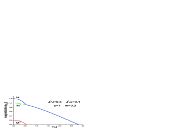
Figure 2: (color online)  Temperature dependence of the ferromagnetic moments: $M$ (blue line)-the magnetization of the system, $M^{l}$ (green line)-contribution of the localized electrons, $M^{it}$ (red line)-contribution of the itinerant electrons for parameters $s=1,\,m=0.2,\,J^{l}/J=0.5,\,J^{it}/J=0.1$: modified spin-wave theory.

The figure shows an anomalous increasing of the magnetization $M$ below $T^{*}$ which is in a very good agrement with the experiment (see Fig.1 2fmp6 ). The present theory enables us to gain insight into the nature of the two phases. In the low temperature phase $(0,T^{*})$, the localized and itinerant electrons contribute to the magnetization of the system, while in the high temperature phase $(T^{*},T_{C})$, only localized electrons form ferromagnetic moment. At first sight, it seems to be counterintuitive because the local moments build an effective magnetic field, which, due to spin-Fermion interaction, leads to finite itinerant electron spin polarization. This is true in the classical limit. In the quantum case, the spin-wave fluctuations suppress the magnetic orders of the itinerant and localized electrons at different temperatures $T^{*}$ and $T_{C}$ as a result of different interactions of the magnon with localized and itinerant electrons. the spin fermion interaction increases the alignment of the local moments, and magnetic order of itinerant electrons is very strong and $T^{*}$ approaches $T_{C}$.

It is well known that the onset of magnetism in the itinerant systems is accompanied with strong anomaly in resistivity 2fmp12 . This phenomena is experimentally observed at $T^{*}$ in the case of $UGe_{2}$ 2fmp4 . This is another support for the theoretical interpretation of $T^{*}$ as a temperature at which the itinerant electrons form ferromagnetic order.

To conclude, we note that to do more precise fitting with experimental values of the Curie temperature, one has to account for the magnon-magnon interaction. However, even the approximate calculations in the present Brief Report capture the main feature of the two-spin ferromagnetic systems and the existence of two phases.

The next step of our investigation is to understand the mechanism of decreasing the phase temperature $T^{*}$. This will help us to understand the origin of the superconductivity in these materials.

This work was financially supported by the Grant-in-Aid for Scientific Research No19340099 from the JSPS. The author is grateful to Prof. Miyake for the kind hospitality and useful discussions.

References

(1) S. S. Saxena, P. Agarwal, K. Ahilan, F. M. Grosche, R.K.W. Haselwimmer, M.J.Steiner,
E.Pugh, I.R.Walker, S. R. Julian, P. Monthoux, G. G. Lonzarich, A.
Huxley, I. Sheikin, D. Braithwaite, and J. Flouquet, Nature
(London) 406, 587 (2000).
(2) A. Huxley, I. Sheikin, E. Ressouche, N. Kernavanois, D. Braithwaite, R. Calemczuk,
and J. Flouquet, Phys. Rev. B 63, 144519 (2001).
(3) N. Tateiwa, T. Kobayashi, K. Hanazono, K. Amaya, Y. Haga, R. Settai,
and Y.Onuki, J. Phys. Condens. Matter 13, L17 (2001).
(4) G. Oomi, K. Nishimura, Y. Onuki, and S.W. Yun, Physica B186-188, 758 (1993).
(5) N. Tateiwa, K. Hanazono, T. C. Kobayashi, K. Amaya, T. Inoue, K. Kindo,
Y. Koike, N. Metoki, Y. Haga, R. Settai, and Y. Onuki, J. Phys. Soc. Jpn 70, 2876 (2001).
(6) C. Pfleiderer and A. D. Huxley, Phys. Rev. Lett., 89, 147005 (2002).
(7) G. Motoyama, S. Nakamura, H. Kadoya, T. Nishioka,
and N. K. Sato,Phys. Rev. B 65, 020510 (2001).
(8) N. Tateiwa, T. C. Kobayashi, K. Amaya, Y. Haga, R. Setta, and Y. Onuki,Phys. Rev. B 69, 180513(R) (2004).
(9) S. Watanabe and K. Miyake, J. Phys. Society of Japan 71, 2489 (2002).
(10) K. G. Sandeman, G. G. Lonzarich, and A. J. Schofield, Phys. Rev. Lett., 90, 167005 (2003).
(11) S. Q. Shen, International Journal of Physics B 12, 709 (1998).