Dynamical Tunneling in Molecules: Quantum Routes to Energy Flow

Abstract

Dynamical tunneling, introduced in the molecular context, is more than two decades old and refers to phenomena that are classically forbidden but allowed by quantum mechanics. The barriers for dynamical tunneling, however, can arise in the momentum or more generally in the full phase space of the system. On the other hand the phenomenon of intramolecular vibrational energy redistribution (IVR) has occupied a central place in the field of chemical physics for a much longer period of time. Despite significant progress in understanding IVR a priori prediction of the pathways and rates is still a difficult task. Although the two phenomena seem to be unrelated several studies indicate that dynamical tunneling, in terms of its mechanism and timescales, can have important implications for IVR. It is natural to associate dynamical tunneling with a purely quantum mechanism of IVR. Examples include the observation of local mode doublets, clustering of rotational energy levels, and extremely narrow vibrational features in high resolution molecular spectra. Many researchers have demonstrated the usefulness of a phase space perspective towards understanding the mechanism of IVR. Interestingly dynamical tunneling is also strongly influenced by the nature of the underlying classical phase space. Recent studies show that chaos and nonlinear resonances in the phase space can enhance or suppress dynamical tunneling by many orders of magnitude. Is it then possible that both the classical and quantum mechanisms of IVR, and the potential competition between them, can be understood within the phase space perspective? This review focuses on addressing the question by providing the current state of understanding of dynamical tunneling from the phase space perspective and the consequences for intramolecular vibrational energy flow in polyatomic molecules.

I Introduction

The field of chemical physics is full of phenomena that occur quantum mechanically, with observable consequences, despite being forbidden by classical mechanicsbmw94 . All such processes are labeled as tunneling with the standard elementary example being that of a particle surmounting a potential barrier despite insufficient energy. However the notion of tunneling is far more general in the sense that the barriers can arise in the phase spacelc79 ; dh81 ; hp84 ; Ozo84 . In other words the barriers are dynamical and arise due to the existence of one or several conserved quantities. Barriers due to exactly conserved quantities i.e., constants of the motion are usually easy to identify. A special case is that of a particle in a one dimensional double well potential wherein the barrier is purely due to the conserved energy. On the other hand it is possible, and frequently observed, that the dynamics of the system can result in one or more approximate constants of the motion which can manifest as barriers. The term approximate refers to the fact that the relevant quantities, although strictly nonconserved, are constant over timescales that are long compared to certain system timescales of interestkuzstubook . Such approximate dynamical barriers are not easy to identify and in combination with the other exact constants of the motion can give rise to fairly complex dynamics. As usual one anticipates that the dynamical barriers will act as bottlenecks for the classical dynamics whereas quantum dynamics will ‘break free’ due to tunneling through the dynamical barriers i.e., dynamical tunneling. However, as emphasized in this review, the situation is not necessarily that straightforward since the mere existence of a finite dynamical barrier does not guarantee that dynamical tunneling will occur. This is especially true in multidimensions since a variety of other dynamical effects can localize the quantum dynamics. In this sense the mechanism of dynamical tunneling is far more subtle as compared to the mechanism of tunneling through nondynamical barriers.

The distinction between energetic and dynamical barriers can be illustrated by considering the two-dimensional Hamiltonian

$$H(x,y,p_{x},p_{y}) = \frac{1}{2}(p_{x}^{2}+p_{y}^{2})+V(x,y)$$ (1)

$$V(x,y) = V_{0}(x^{2}-a^{2})^{2}+\frac{1}{2}\omega^{2}y^{2}+\gamma x^{2}y^{2}$$

which represents a one-dimensional double well (in the $x$ degree of freedom) coupled to a harmonic oscillator (in the $y$ degree of freedom). For energies $E$ below the barrier height $V_{b}=V_{0}a^{4}$, the $y=0$ Poincaré surface of section in Fig. 1 shows two disconnected regions in the phase space. This reflects the fact that the corresponding isoenergetic surfaces are also disconnected. Thus one speaks of an energetic barrier separating the left and the right wells. On the other hand Fig. 1 shows that for $E>V_{b}$ the Poincaré surface of section again exhibits two regular regions related to the motion in the left and right wells despite the absence of the energetic barrier. In other words the two regions are now part of the same singly connected energy surface but the left and the right regular regions are separated by dynamical barriers. The various nonlinear resonances and the chaotic region seen in Fig. 1 should be contrasted with the phase space of the one-dimensional double well alone which is integrable. Later in this review examples will be shown wherein there are only dynamical barriers and no static potential barriers. Note that in higher dimensions, see discussions towards the end of this secion, one does not even have the luxury of visualizing the global phase space, as in Fig. 1, let alone identifying the dynamical barriers!

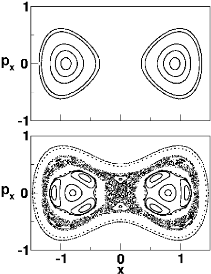
Figure 1: Poincaré surface of section for the example two-dimensional potential in Eq. (1). The parameter values are chosen to be $V_{0}=0.25$, $a=\omega=\gamma=1$ and the static barier height is therefore $V_{b}=0.25$. The surface of section are defined by $y=0$ and $p_{y}>0$. The top panel shows the phase space for $E=0.2$ (below the static barrier height) and one observes two disconnected regular regions separated by energetic barrier. The bottom panel corresponds to $E=0.4$ (above the static barrier height) and shows the left and right regular regions separated now only by dynamical barriers. Model system and parameters taken from ref. Schl06, .

In the case of multidimensional tunneling through potential barriers it is now well established that valuable insights can be gained from the phase space perspectivebm72 ; Mil74 ; Wil86 ; Hel99 ; sc06 It is not necessary that tunneling is associated with transfer of an atom or group of atoms from one site to another siteHel01 . One can have, for instance, vibrational excitations transferring from a particular mode of a molecule to a completely different modeHel99 ; Hel95 . Examples like Hydrogen atom transfer and electron transfer belong to the former class whereas the phenomenon of intramolecular vibrational energy redistribution (IVR) is associated with the latter classHel95 . In recent years dynamical tunneling has been realized in a number of physical systems. Examples include driven atomszdb98 ; bdz02 , microwavedghhrr00 or optical cavitiesns97 , Bose-Einstein condensateshetal01 ; sor01 , and in quantum dotsbafmli03 . Thinking of dynamical tunneling as a close cousinHel99 ; Hel01 of the “above barrier reflection” (cf. example shown in Fig. 1) a recent papergutk05 by Giese et al. suggests the importance of dynamical tunneling in order to understand the eigenstates of the dichlorotropolone molecule. This review is concerned with the molecular manifestations of dynamical tunneling and specifically on the relevance of dynamical tunneling to IVR and the corresponding signatures in molecular spectra. One of the aims is to reveal the detailed phase space description of dynamical tunneling. This, in turn, leads to the identification of the key structures in phase space and a universal mechanism for dynamical tunneling in all of the systems mentioned above.

In IVR studies, which is of paramount interest to chemical dynamics, one is interested in the fate of an initial nonstationary excitation in terms of timescales, pathways and destinationslsp94 ; gb98 ; Gru00 ; mq01 ; gw04 . Will the initial energy “hot-spot” redistribute throughout the molecule statistically? Alternatively, to borrow a term from a recent reviewGru03 , is the observed statisticality only “skin-deep”? The former viewpoint is at the heart of one of the most useful theories for reaction rates - the RRKM (Rice-Rampsperger-Kassel- Marcus) theorybaerhasebook . On the other hand, recent studiesgsh03 seem to be leaning more towards the latter viewpoint. As an aside it is worth mentioning that IVR in molecules is essentially the FPUfpu55 ; crz05 (Fermi-Pasta-Ulam) problem; only now one needs to worry about a multidimensional network of coupled nonlinear oscillators. In a broad sense, the hope is that a mechanistic understanding of IVR will yield important insights into mode-specific chemistry and the coherent control of reactions. Consequently, substantial experimentalGru00 ; nf96 ; kp00 and theoretical effortsRice81 ; Uzer91 ; Ezra98 have been directed towards understanding IVR in both time and frequency domains. Most of the studies, spanning many decades, have focused on the gas phase. More recently, researchers have studied IVR in the condensed phase and it appears that the gas phase studies provide a useful starting point. A detailed introduction to the literature on IVR is beyond the scope of the current article. A brief description is provided in the next section and the reader is refered to the literature below for a comprehensive account of the recent advances. The reviewnf96 by Nesbitt and Field gives an excellent introduction to the literature. The reviewGru04 by Gruebele highlights the recent advances and the possibility of controlling IVR. The topic of molecular energy flow in solutions has been recently reviewedaka03 by Aßmann, Kling and Abel.

Tunneling leads to quantum mixing between states localized in classically disconnected regions of the phase space. In this general setting barriers arise due to exactly or even approximately conserved quantities. Thus, for example, it is possible for two or more localized quantum states to mix with each other despite the absence of any energetic barriers separating them. This has significant consequences for IVR in isolated moleculesHel95 since energy can flow from an initially excited mode to other, qualitatively different, modes; classically one would predict very little to no energy flow. Hence it is appropriate to associate dynamical tunneling with a purely quantum mechanism for energy flow in molecules. In order to have detailed insights into IVR pathways and rates it is necessary to study both the classical and quantum routes. The division is artificial since both mechanisms coexist and compete with each other. However, from the standpoint of control of IVR deciding the importance of one route over the other can be useful. In molecular systems the dynamical barriers to IVR are related to the existence of the so called polyad numbersfe87 ; Kell90 . Usually the polyad numbers are quasiconserved quantities and act as bottlenecks for energy flow between different polyads. Dynamical tunneling, on the otherhand, could lead to interpolyad energy flow. Historically the time scales for IVR via dynamical tunneling have been thought to be of the order of hundreds of picoseconds. However recent advances in our understanding of dynamical tunneling suggest that the timescales could be much smaller in the mixed phase space regimes. This is mainly due to the observationsTom01 that chaos in the underlying phase space can enhance the tunneling by several orders of magnitude. Conversely, very early on it was thought that the extremely long timescales would allow for mode-specific chemistry. Presumably the chaotic enhancement would spoil the mode specificty and hence render the initially prepared state unstable. Thus it is important to understand the effect of chaos on dynamical tunneling in order to suppress the enhancement.

Obtaining detailed insights into the phenomenon of dynamical tunneling and the resulting consequences for IVR requires us to address several questions. How does one identify the barriers? Can one explicitly construct the dynamical barriers for a given system? What is the role of the various phase space structures like resonances, partial barriers due to broken separatrices and cantori, and chaos? Which, if any, of the phase space structures provide for a universal description and mechanism of dynamical tunneling? Finally the most important question: Do experiments encode the sensitivity of dynamical tunneling to the nature of the phase space? This review is concerned with addressing most of the questions posed above in a molecular context. Due to the nature of the issues involved considerable work has been done by the nonlinear physics community and in this work some of the recent developements will be highlighted since they can have significant impact on the molecular systems as well. Another reason for bringing together developements in different fields has to do with the observation that the literature on dynamical tunneling and its consequences are, curiuosly enough, disjoint with hardly any overlap between the molecular and the ‘non’ molecular areas.

At this stage it is important and appropriate, given the viewpoint adopted in this review, to highlight certain crucial issues pertaining to the nature of the classical phase space for systems with several ($N\geq 3$) degrees of freedom. A significant portion of the present review is concerned with the phase space viewpoint of dynamical tunneling in systems with $N\leq 2$. The last section of the review discusses recent work on a model with three degrees of freedom. The sparsity of work in $N\geq 3$ is not entirely surprising and parallels the situation that prevails in the classical-quantum correspondence studies of IVR in polyatomic molecules. Indeed it will become clear from this review that classical phase space structures are, to a large extent, responsible for both classical and quantum mechanisms of IVR. Thus, from a fundamental, and certainly from the molecular, standpoint it is highly desirable to understand the mechanism of classical phase space transport in systems with $N\geq 3$. In the early eighties the seminal workmmp84 by Mackay, Meiss, and Percival on transport in Hamiltonian systems with $N=2$ motivated researchers in the chemical physics community to investigate the role of various phase space structures in IVR dynamics. In particular these studiesDav85 ; dg86 ; gr87 ; ml89 ; sd88 helped in providing a deeper understanding of the dynamical origin of nonstatistical behaviour in molecules. However molecular systems typically have atleast $N=3$ and soon the need for a generalization to higher degrees of freedom was felt; this task was quite difficult since the concept of transport across broken separatrices and cantori do not have a straightforward generalization in higher degrees of freedom. In addition tools like the Poincaré surface of section cease to be useful for visualizing the global phase space structures. WigginsWigg90 provided one of the early generalizations based on the concept of normally hyperbolic invariant manifolds (NHIM) which led to illuminating studiesge91 ; almm90 in order to elucidate the dynamical nature of the intramolecular bottlenecks for $N\geq 3$. Although useful insights were gained from several studiesge91 ; almm90 ; grd86 ; mde87 ; tr88 ; lmt91 ; Leo91 the intramolecular bottlenecks could not be characterized at the same levels of detail as in the two degree of freedom cases. It is not feasible to review the various studies and their relation/consequences to the topic of this article. The reader is referred to the paperge91 by Gillilan and Ezra for an introduction and to the monographwigbook by Wiggins for an exposition to the theory of NHIMs. Following the initial studies, which were perhaps ahead of their time, far fewer efforts were made for almost a decade but there has been a renewal of interest in the problem over the last few years with the NHIMs playing a crucial role. Armed with the understanding that the notion of partial barriers, chaos, and resonances are very different in $N\geq 3$ fresh insights on transition state and RRKM theories, and hence IVR, are beginning to emergewwju01 ; ujpyw02 ; wbw04 ; sclu04 ; acp130 ; bhc05 ; wbw05 ; gkmr05 ; bhc06 ; sblkt06 ; sk06 ; slkt07 .

To put the issues raised above in perspective for the current review note that there are barriers in phase space through which dynamical tunneling occurs and at the same time there are barriers that can also lead to the localization of the quantum dynamics. The competition between dynamical tunneling and dynamical localization is already important for systems with $N=2$ and this will be briefly discussed in the later sections. Towards the end of the review some work on a three degrees of freedom model are presented. However, as mentioned above, the ideas are necessarily preliminary since to date one does not have a detailed understanding of either the classical barriers to transport nor the dynamical barriers which result in dynamical tunneling. Naturally, the competition between them is an open problem. We begin with a brief overview of IVR and the explicit connections to dynamical tunneling.

I.1 State space model of IVR

Consider a molecule with $N$ atoms which has $s\equiv 3N-6$ ($3N-5$ for linear molecules) vibrational modes. Dynamical studies, classical and/or quantum, require the $s$-dimensional Born-Oppenheimer potential energy surface $V(Q_{1},Q_{2},\ldots,Q_{s})$ in terms of some convenient generalized coordinates ${\bf Q}$ and their choice is a crucial issue. Obtaining the global $V({\bf Q})$ by solving the Schrödinger equation is a formidable task even for mid-sized molecules. Traditionally, therefore, a perturbative viewpoint is adopted which has enjoyed a considerable degree of success. For example, near the bottom of the well and for low levels of excitations the approximation of vibrations by uncoupled harmonic normal modes is sufficient and the molecular vibrational Hamiltonian can be expressed perturbatively asbrionfieldbook ; papalibook :

$$H=\sum_{i=1}^{s}\frac{\omega_{i}}{2}(P_{i}^{2}+Q_{i}^{2})+\sum_{ijk=1}^{s}\phi_{ijk}Q_{i}Q_{j}Q_{k}+\ldots$$ (2)

In the above $({\bf P},{\bf Q})$ are the dimensionless vibrational momenta and normal mode coordinates respectively. The deviations from the harmonic limit are captured by the anharmonic terms with strengths $\{\phi_{ijk}\}$. Such small anharmonicities account for the relatively weak overtone and combination transitions observed in experimental spectra. However with increasing energy the anharmonic terms become important and doubts arise regarding the appropriateness of a perturbative approach. The low energy normal modes get coupled and the very concept of a mode becomes ambiguous. There exists sufficient evidenceiffjkbs99 ; jf00 ; jb80 ; kt07 for the appearance of new ‘modes’, unrelated to the normal modes, with increasing vibrational excitations. Nevertheless detailed theoretical studies over the last couple of decades has shown that it is still possible to understand the vibrational dynamics via a suitably generalized perturbative approach - the canonical Van-Vleck perturbation theory (CVPT)Van51 ; js02 ; ms00 . The CVPT leads to an effective or spectroscopic Hamiltonian which can be written down as

$$\widehat{H}=\widehat{H}_{0}({\bf n})+V({\hat{\bf a}},{\hat{\bf a}^{\dagger}})$$ (3)

where $\hat{\bf n}\equiv\hat{\bf a}^{\dagger}\hat{\bf a},\hat{\bf a}$, and $\hat{\bf a}^{\dagger}$ are the harmonic number, destruction and creation operators. The zeroth-order part i.e., the Dunham expansionDun32

$$\widehat{H}_{0}({\bf n})=\sum_{j}\omega_{j}\hat{N}_{j}+\sum_{i\geq j}x_{ij}\hat{N}_{i}\hat{N}_{j}+\ldots$$ (4)

is diagonal in the number representation. In the above expression $\hat{N}_{j}\equiv\hat{n}_{j}+d_{j}/2$ with $n_{j}$ being the number of quanta in the j^th mode with degeneracy $d_{j}$. The off-diagonal terms i.e., anharmonic resonances have the form

$$V({\hat{\bf a}},{\hat{\bf a}^{\dagger}})=\sum_{\bf m}\prod_{j}\Phi_{\bf m}(a_{j}^{\dagger})^{m_{j}^{+}}(a_{j})^{m_{j}^{-}}\equiv\sum_{\bf m}V_{\bf m}(\hat{\bf a},\hat{\bf a}^{\dagger})$$ (5)

with ${\bf m}=\{m_{1}^{\pm},m_{2}^{\pm},\ldots\}$. These terms represent the couplings between the zeroth-order modes and are responsible for IVR starting from a general initial state $|\Psi\rangle=\sum_{j}c_{{\bf n}j}|{\bf n}\rangle$.

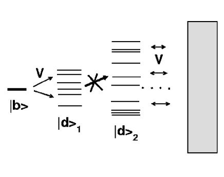
Figure 2: Schematic diagram illustrating the tier model of IVR. The bright state $|b\rangle$ is coupled to the various dark states sorted into tiers through perturbations $V$. As an example this sketch indicates fast IVR between $|b\rangle$ and states in $|d\rangle_{1}$ whereas further flow of energy to states $|d\rangle_{2}$ in the second tier is restricted due to the lack of couplings. Nevertheless it is possible that vibrational superexchange can couple the first and second tiers and energy can eventually flow into the final tier (grey) over long timescales.

A few key points regarding the effective Hamiltonians can be noted at this juncture. There are two routes to the effective Hamiltonians. In the CVPT method the parameters of the effective Hamiltonian are related to the original molecular parameters of $V({\bf Q})$. The other route, given the difficulties associated with determining a sufficiently accurate $V({\bf Q})$, is via high resolution spectroscopy. The parameters of Eq.(3) are determinedbrionfieldbook by fitting the experimental data on line positions and, to a lesser extent, intensities. The resulting effective Hamiltonian is only a model and hence the parameters of the effective Hamiltonian do not have any obvious relationship to the molecular parameters of $V({\bf Q})$. Although the two routes to Eq.(3) are very different, they complement one another and each has its own advantages and drawbacks. The reader is refered to the reviews by Sibert and Joyeux for a detailed discussion of the CVPT approach. The reviewiffjkbs99 by Ishikawa et al. on the experimental and theoretical studies of the HCP $\leftrightarrow$ CPH isomerization dynamics provides, amongst other things, a detailed comparison between the two routes.

Imagine preparing a specific initial state, say an eigenstate of $H_{0}$, denoted as $|{\bf b}\rangle$. Theoretically one is not restricted to $|{\bf b}\rangle$ and very general class of initial states can be considered. However, time domain experiments with short laser pulses excite specific vibrational overtone or combination states, called as the zeroth-order bright states (ZOBS), which approximately correspond to the eigenstates of $H_{0}$. The rest of the optically inaccessible states are called as dark states $\{|{\bf d}\rangle\}$. Here the zeroth-order eigenstates $|{\bf n}\rangle$ are partitioned as $\{|{\bf b}\rangle,|{\bf d}\rangle_{1},|{\bf d}\rangle_{2},\ldots\}$. The perturbations $V({\bf a},{\bf a}^{\dagger})$ couple the bright state with the dark states leading to energy flow and impose a hierarchical coupling structure between the ZOBS and the dark states. Thus one imagines, as shown in Fig. 2, the dark states to be arranged in tiers, determined by the order $p=\sum_{j}(m^{+}_{j}+m^{-}_{j})$ of the $V_{\bf m}$, with an increasing density of states across the tiers. This implies that the the local density of states around $E_{\bf b}^{0}$ is the important factor and experiments do point to a hierarchical IVR processlsp94 . For example, Callegari et al. have observed seven different time scales ranging from 100 femtoseconds to 2 nanoseconds for IVR out of the first CH stretch overtone of the benzene moleculecsmlsd97 . Gruebele and coworkers have impressively modeled the IVR in many large molecules based on the hierarchical tiers conceptgb98 . In a way the coupling $V({\bf a},{\bf a}^{\dagger})$ imposes a tier structure on the IVR; similar tiered IVR flow would have been observed if one had investigated the direct dynamics ensuing from the global $V({\bf Q})$. Thus the CVPT and its classical analog help in unraveling the tier structure. Nevertheless dominant classical and quantum energy flow routes still have to be identified for detailed mechanistic insights.

In the time domain the survival probability

$$P_{\bf b}(t)=|\langle{\bf b}(0)|{\bf b}(t)\rangle|^{2}=\sum_{\alpha,\beta}p_{{\bf b}\alpha}p_{{\bf b}\beta}e^{-i(E_{\alpha}-E_{\beta})t/\hbar}$$ (6)

gives important information on the IVR process. The eigenstates of the full Hamiltonian have been denoted by $|\alpha\rangle,|\beta\rangle,\ldots$ with $p_{{\bf b},\alpha}=|\langle\alpha|{\bf b}\rangle|^{2}$ being the spectral intensities. The long time average of $P_{\bf b}(t)$

$$\sigma_{\bf b}=\lim_{T\rightarrow\infty}\frac{1}{T}\int_{0}^{T}P_{\bf b}(t)dt=\sum_{\alpha}p_{{\bf b},\alpha}^{2}$$ (7)

is known as the inverse participation ratio (also called as the dilution factor in the spectroscopic community). Essentially $\sigma_{\bf b}^{-1}$ indicates the number of states that participate in the IVR dynamics out of $|{\bf b}\rangle$.

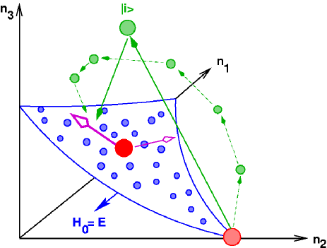
Figure 3: (Colour online) Schematic diagram illustrating the state space model of IVR. Zeroth order states on the energy shell (blue circles) and off the energy shell (green circles) are indicated. An interior state (large red circle) can couple to nearby states via several anharmonic resonances indicated by purple arrows. Edge states (shaded red circle) can couple via off-resonant virtual states $|i_{\alpha}\rangle$ to states on the energy shell. Examples of such one-step and multistep superexchange paths in the state space are shown.

Although the tier picture has proved to be useful in analysing IVR, recent studiesGru00 ; sw92 ; sw95 ; sww95 ; sww96 emphasize the far greater utility in visualising the IVR dynamics of $|{\bf b}(t)\rangle$ as a diffusion in the zeroth-order quantum number space or state space denoted by $(n_{1},n_{2},\ldots,n_{s})$. The state space picture, shown schematically in Fig. 3, highlights the local nature and the directionality of the energy flow due to the various anharmonic resonances. In the “one-dimensional” tier scheme shown in Fig. 2 the anisotropic nature of the IVR dynamics is hard to discern. Tiers in the state space are formed by zeroth-order states within a certain distance from the bright state and hence still organized by the order of the coupling resonances. In the long time limit most states that participate in the IVR dynamics are confined, due to the quasi-microcanonical nature of the laser excitation, to an energy shell $E^{0}_{b}\pm\delta E$ with $E^{0}_{b}$ being the bright state energy. The IVR dynamics occurs on a $D$-dimensional subspace, refered to as the IVR “manifold”, of the state space due to the local nature of the couplings between $|{\bf b}\rangle$ and ${|{\bf d}_{j}\rangle}$ with $H\approx E^{0}_{b}\approx E^{0}_{d_{j}}$. One of the key prediction of the state space model is that the survival probability exhibits a power law at intermediate timesgw04 ; wg99

$$P_{\bf b}(t)\sim\sigma_{\bf b}+(1-\sigma_{\bf b})\left[1+\frac{2t}{\tau D}\right]^{-D/2}$$ (8)

with $D\ll 3N-6$, the number of vibrational modes of the molecule. Thus the effective dimensionality $D$ of the IVR manifold in the state space can be fairly small and a large body of work in the recent years support the state space viewpointGru00 ; gw04 ; aka03 . The effective dimensionality itself is crucially dependent on the extent to which classical and quantum mechanisms of IVR manifest themselves at specific energies. One possible interpretation of $D$ is as follows. If $D\approx 3N-6$ then the dynamics in the state space can be thought of as a normal diffusive process and thus ergodic over the state space. In such a limit for large $N$ (molecules) the survival can be well approximated by an exponential behaviour. For $D\ll 3N-6$ the IVR dynamics is anisotropic and the dynamics is nonergodic with $D$ typically being nonintegral. Note that the terms “manifold” and “effective dimensionality” are being used a bit loosely since one does not have a very clear idea of the topology of the IVR manifold as of yet.

Leitner and Wolynes, building upon the earlier work of Logan and Wolyneslow90 , have provided criterialw96jcp for vibrational state mixing and energy flow from the state space perspective. Using a local random matrix approach to the Hamiltonian in Eq. (3) the rate of energy flow out of $|{\bf b}\rangle$ is given by

$$k(E)=\frac{2\pi}{\hbar}\sum_{Q}K_{Q}\langle|\psi_{Q}|^{2}\rangle D_{Q}(E)$$ (9)

with $Q$ being a distance in the state space. The term $\langle|\psi_{Q}|\rangle$ represents the average effective coupling of $|{\bf b}\rangle$ to the states, $K_{Q}$ of them with density $D_{Q}(E)$, a distance $Q$ away in state space. The extent of state mixing is characterized by the transition parameter

$$T(E)=\frac{2\pi}{3}\left(\sum_{Q}K_{Q}\langle|\psi_{Q}|\rangle D_{Q}(E)\right)^{2}$$ (10)

and the transition between localized and extended states is located at $T(E)=1$. The key term is the effective coupling $\psi_{Q}$ which involves both low and high order resonances. Applications to several systems shows that the predictions based on Eq. (9) and Eq. (10) are both qualitatively and quantitativelylw97 accurate.

I.2 Connections to dynamical tunneling

The perspective of IVR being a random walk on an effective $D$-dimensional manifold in the quantum number space is reasonableGru00 ; sw92 as long as direct anharmonic resonances exist which connect the bright state with the dark states. It is useful to emphasize again that the existence of direct anharmonic resonances in itself does not imply ergodicity over state space i.e., the random walk need not be normal. What happens if, for certain bright states, there are no direct resonances available? In other words, the coupling matrix elements $\langle{\bf d}_{j}|V|{\bf b}\rangle\approx 0$ for all $j$. What would be the mechanism of IVR, if any, in such cases? Examples of such states in fact correspond to overtone excitations which are typically prepared in experiments. The overtone states are also called as edge states from the state space viewpoint since most of the excitation is localized in one single mode of the molecule. Thus, for example, in a system with four degrees of freedom a state $|{\bf b}\rangle\equiv|n_{1},0,0,0\rangle$ would be called as an edge state whereas the state $|n_{1},0,n_{3},n_{4}\rangle$, corresponding to a combination state, is called as an interior state. The edge states, owing to their location in the state space, have fewer anharmonic resonances available for IVR as compared to the interior states. To some extent such a line of reasoning leads one to anticipate overtone excitations to have slower IVR when compared to the combination states. A concrete example comes from the theoretical work of Holme and Hutchinson wherein the dynamics of overtone excitations in a model system representing coupled CH-stretch and CCH-bend interacting with an intense laser field was studiedhh86 ; Hut89 . They found that classical dynamics predicted no significant energy flow from the high overtone excitations. However the corresponding quantum calculations did indicate significant IVR. Based on their studies Holme and Hutchinson concluded that overtone absorption proceeds via dynamical tunneling on timescales of the order of a few nanoseconds.

Experimental evidence for the dynamical tunneling route to IVR was provided in a series of elegant worksklmps91 ; gtls93 by the Princeton group. The frequency domain experiments involved the measurement of IVR lifetimes of the acetylinic CH-stretching states in (CX₃)₃YCC$\equiv$H molecules with X$=$H,D and Y$=$C,Si. The homogeneous line widths, which are related to the rate of IVR out of the initial nonstationary state, arise due to the vibrational couplings between the CH-stretch and the various other vibrational modes of the molecule. Surprisingly Kerstel et al. foundklmps91 extremely narrow linewidths of the order of 10^-1 - 10^-2 cm^-1 which translate to timescales of the order of thousands of vibrational periods of the CH-stretching vibration. Thus the initially prepared CH-stretch excitation remains localized for extremely long times. Such long IVR timescales were ascribed to the lack of strong/direct anharmonic resonances coupling the CH-stretch with the rest of the molecular vibrations. The lack of resonances, despite a substantial density of states, combined with IVR timescales of several nanoseconds implies that the mechanism of energy flow is inherently quantum. Another studyglls94 by Gambogi et al. examines the possibility of long range resonant vibrational energy exchange between equivalent CH-stretches in CH₃Si(C$\equiv$CH)₃. There have been several experimentsfcsk88 ; mn89 ; mmp92 ; gp92 ; uctc95 that indicate multiquantum zeroth-order state mixings due to extremely weak couplings of the order of 10^-1 - 10^-2 cm^-1 in highly vibrationally excited molecules.

Since the early work by Kerstel et al. other experimental studies have revealed the existence of the dynamical tunneling mechanism for IVR in large organic molecules. For instance in a recent workcpcesgls03 Callegari et al. performed experimental and theoretical studies on the IVR dynamics in pyrrole (C₄H₄NH) and 1,2,3-triazine (C₃H₃N₃). Specifically, they chose the initial bright states to be the edge state $2\nu_{14}$ CH-stretch for pyrrole and the interior state $\nu_{6}^{1}+2\nu_{7}^{2}$ corresponding to the CH stretching-ring breathing combination for triazine. In both cases very narrow IVR features, similar to the observations by Kerstel et al., were seen in the spectrum. This pointed towards an important role of the off-resonant states to the observed and calculated narrow IVR features. The analysis by Callegari et al. reveals that near the IVR threshold it is reasonable to expect such highly off-resonant coupling mechanisms to be operative. Another example for the possible existence of the off-resonant mechanism comes from the experimentprb04 by Portonov, Rosenwaks, and Bar wherein the IVR dynamics ensuing from $2\nu_{1}$, $3\nu_{1}$, and $4\nu_{1}$ CH-acetylinic stretch of 1-butyne are studied. It was found that the homogeneous linewidth of the $4\nu_{1}$ state, $\sim$ 0.5 cm^-1, is about a factor of two smaller than the widths of $2\nu_{1}$ and $3\nu_{1}$.

It is important to note that the involvement of such off-resonant states can occur at any stage of the IVR process from a tier perspective. In other words it is possible that the bright state undergoes fast initial IVR due to strong anharmonic resonances with states in the first tier but the subsequent energy flow might be extremely slow. Several experiments point towards the existence of such unusually long secondary IVR time scales which might have profound consequences for the interpretation of the high resolution spectra. Boyarkin and Rizzo demonstratedbr96 the slow secondary time scales in their experiments on the IVR from the alkyl CH-stretch overtones of CF₃H. Upon excitation of the CH-stretch fast IVR occurs to the CH stretch-bend combination states on femtosecond timescales. However the vibrational energy remains localized in the mixed stretch-bend states and flows out to the rest of the molecule on timescales of the order of hundred picoseconds. Similar observations were madelbspr96 by Lubich et al. on the IVR dynamics of OH-stretch overtone states in CH₃OH.

The interpretation of the above experimental results as due to dynamical tunneling is motivated by the theoretical analysis by Stuchebrukhov and Marcus in a landmark papersm93 . In the initial work they explained the narrow features, observed in the experimentsklmps91 by Kerstel et al., by invoking the coupling of the bright states with highly off-resonant gateway states which, in turn, couple back to states that are nearly isoenergetic with the bright state. In Fig. 3 an example of the indirect coupling via a state which is off the energy shell in the state space is illustrated. More importantly Stuchebrukhov and Marcus argued that the mechanism, described a little later in this review and anticipated earlier by Hutchinson, Sibert, and Hyneshsh84 , involving high order coupling chains is essentially a form of generalized tunnelingsm932 . Hence one imagines dynamical barriers which act to prevent classical flow of energy out of the initial CH-stretch whereas quantum dynamical tunneling does lead to energy flow, albeit very slowly. Similar arguments had been put forward by Hutchinson demonstratingHut84 the importance of the off-resonant coupling leading to the mixing of nearly degenerate high energy zeroth-order states in cyanoacetylene HCC$\equiv$CN. It was argued that such purely quantum relaxation pathway would explain the observed broadening of the overtone bands in various substituted acetylenes.

The above examples highlight the possible connections between IVR and dynamical tunneling. However it was realized very early on that observations of local mode doubletslc80 ; lc81 ; lc82 in molecular spectra and the clustering of rotational energy sublevels with high angular momentahp84 can also be associated with dynamical tunneling. Indeed much of our understanding of the phenomenon of dynamical tunneling in the context of molecular spectra comes from these early works. One of the key feature of the analysis was the focus on a phase space description of dynamical tunneling i.e., identifying the disconnected regions in the phase space and hence classical structures which could be identified as dynamical barriers. Thus the mechanism of dynamical tunneling, confirmed by computing the splittings based on specific phase space structures, could be understood in exquisite detail. However such detailed phase space analysis are exceedingly difficult, if not impossible, for large molecules. For example in the case of the (CX₃)₃YCCH system there are $3N-6=42$ vibrational degrees of freedom. Any attempt to answer the questions on the origin and location of the dynamical barriers in the phase space is seemingly a futile excercise. It is therefore not surprising that Stuchebrukhov and Marcus, although aware of the phase space perspective, provided a purely quantum explanation for the IVR in terms of the chain of off-resonant statessm93 .

Thus one cannot help but ask if the phase space viewpoint is really needed. The answer is affirmative and many reasons can be provided that justify the need and utility of a phase space viewpoint. First, as noted by HellerHel95 ; Hel99 , the concept of tunneling is meaningless without the classical mechanics of the system as a baseline. In other words, in order to label a process as purely quantum it is imperative that one establishes the absence of the process within classical dynamics. Note that for dynamical tunneling it might not be easy to a priori make such a distinction. There are mechanisms of classical transport, especially in systems with three or more degrees of freedom, involving long timescales which might give an impression of a tunneling process. It is certainly not possible to differentiate between classically allowed and forbidden mechanisms by studying the spectral intensity and splitting patterns alone due to the nontrivial role played by the stochasticity in the classical phase space. Secondly, the quantum explanation is in essence a method to calculate the contribution of dynamical tunneling to the IVR rates in polyatomic molecules. In order to have a complete qualitative picture of dynamical tunneling it is necessary, as emphasised by Stuchebrukhov and Marcussm932 , to find an explicit form of the effective dynamical potential in the state space of the molecule. Third reason, mainly due to the important insights gained from recent studies, has to do with the sensitivity of dynamical tunneling to the stochasticity in the phase spaceTom01 . Chaos can enhance as well as supress dynamical tunneling and for large molecules the phase space can be mixed regular-chaotic even at energies corresponding to the first or second overtone levels. Undoubtedly the signatures should be present in the splitting and intensity patterns in a high resolution spectrum. However the precise mechanism which governs the substantial enhancement/suppression of dynamical tunneling, and perhaps IVR rates is not yet clear. Nevertheless recent developements indicate that a phase space approach is capable of providing both qualitative and quantitative insights into the problem.

A final argument in favor of a phase space perspective needs to be mentioned. It might appear that the dimensionality issue is not all that restrictive for the quantum studies a la Stuchebrukhov and Marcus. However it will become clear from the discussions in the later sections that in the case of large systems even calculating, for example local mode splittings via the minimal perturbative expression in Eq. (56) can be prohibitively difficult. One might argue that a clever basis would reduce the number of perturbative terms that need to be considered or alternatively one can look for and formulate criteria that would allow for a reliable estimate of the splitting. Unfortunately, a priori knowledge of the clever basis or the optimal set of terms to be retained in Eq. (56) implies a certain level of insight into the dynamics of the system. The main theme of this article is to convey the message that such insights truly originate from the classical phase space viewpoint. With the above reasons in mind the next section provides brief reviews of the earlier approaches to dynamical tunneling from the phase space perspective. This will then set the stage to discuss the more recent advances and the issues involved in the molecular context.

II Dynamical tunneling: early work from the phase space perspective

In a series of pioneering paperslc80 ; lc81 ; lc82 , nearly a quarter of a century ago, Lawton and Child showed that the experimentally observed local mode doublets in H₂O could be associated with a generalized tunneling in the momentum space. In molecular spectroscopy it was appreciated from very early on that highly excited spectra associated with X-H stretching vibrations are better described in terms of local modes rather than the conventional normal modesHal98 ; Jen00 ; hk02 . In a zeroth-order description this corresponds to very weakly coupled, if not uncoupled, anharmonic oscillators. Every anharmonic oscillator, modelled by an appropriate Morse function, represents a specific local stretching mode of the molecule. The central question that Lawton and Child asked was that to what extent are the molecular vibrations actually localized in the individual bonds (local modes)? Analyzing the classical dynamics on the Sorbie-Murrell potential energy surface for H₂O, focusing on the two local O-H stretches, it was found that a clear distinction between normal mode and local mode behaviour could be observed in the phase space. The classical phase space at appropriate energies revealedlc79 two equivalent but classically disconnected regions as a signature of local mode dynamics. Lawton and Child immediately noted the topological similarity between their two dimensional Poincaré surface of section and the phase space of a one dimensional symmetric double well potential. However they also noted that the barrier was in momentum space and hence the lifting of the local mode degeneracy was due to a generalized tunneling in the momentum space. Detailed classicallc79 , quantumlc80 , and semiclassicallc81 investigations of the system allowed Lawton and Child to provide an approximate formula for the splitting $\Delta E_{nm}$ between two symmetry related local mode states $|nm^{\pm}\rangle$ as:

$$\Delta E_{nm}=\frac{2\hbar\bar{\omega}_{nm}}{\pi}\exp\left(-\frac{1}{\hbar}\int_{{\cal C}}|{\bf P}|\cdot d{\bf Q}\right)$$ (11)

The variables $({\bf P},{\bf Q})$ correspond to the mass-weighted momenta and coordinateslc79 ; lc80 . It is noteworthy that Lawton and Child realized, correctly, that the frequency factor $\hbar\bar{\omega}_{nm}$ should be evaluated at a fixed total quantum number $v=n+m$. However the choice of the tunneling path ${\cal C}$ proved to be more difficult. Eventually ${\cal C}$ was taken to be a one dimensional, nondynamical path in the two dimensional coordinate space of the symmetric and antisymmetric normal modes. Although Eq. (11) correctly predicts the trend of decreasing $\Delta E_{nm}$ for increasing $m$ and fixed $n$, the origin and properties of the dynamical barrier remained unclear.

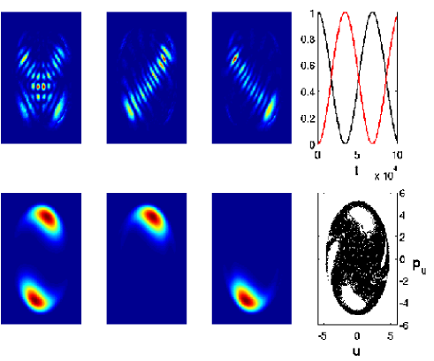
Figure 4: (Colour online) An example of the local mode doublet in the Davis-Heller system. In (a) the $(s,u)$ space representation of the even state ($E=13.589216$) is shown. In (b) and (c) the linear combination $\psi_{\pm}=(\phi_{1}\pm\phi_{2})/\sqrt{2}$ are shown. Right below the configuration space representations the corresponding phase space Husimi representations in the $(u,p_{u})$ Poincaré surface of section are shown. The rightmost figure on the top panel shows the dynamical tunneling occuring when starting with the initial nonstationary state $\psi_{+}$. The period of the oscillations is consistent with the splitting $\Delta E\approx 9.125\times 10^{-5}$. The rightmost figure in the bottom panel shows the $(u,p_{u})$ surface of section.

The analysis by Lawton and Child, although specific to the vibrational dynamics of H₂O, suggested that the phenomenon of dynamical tunneling could be more general. This was confirmed in an influential paper by Davis and Heller wherein it was argued that dynamical tunneling could have significant effects on bound states of polyatomic moleculesdh81 . Incidentally, the word dynamical tunneling was first introduced by Davis and Heller. This work is remarkable in many respects and provided a fairly detailed correspondencedh84 between dynamical tunneling and the structure of the underlying classical phase space for the Hamiltonian $H(s,p_{s},u,p_{u})=(p_{s}^{2}+p_{u}^{2})/2+V(s,u)$. Specifically, the analysis was done on the following two-dimensional potential:

$$V(s,u)=\frac{1}{2}(\omega_{s}^{2}s^{2}+\omega_{u}^{2}u^{2})+\lambda u^{2}s$$ (12)

The system has a discrete symmetry $V(s,-u)=V(s,u)$. For the specific choice of parameter values $\omega_{s}=1.0,\omega_{u}=1.1$, $\lambda=-0.11$, and $\hbar=1$ the dissociation energy is equal to $15.125$ and the potential supports about $115$ bound states. At low energies no doublets are found. However above a certain energy, despite the lack of an energetic barrier, near-degenerate eigenstates $\phi_{1},\phi_{2}$ were observed with small splittings $\Delta E$. In analogy with the symmetric double well system, linear combinations $\psi_{\pm}=(\phi_{1}\pm\phi_{2})/\sqrt{2}$ yielded states localized in the configuration space $(s,u)$. One such example is shown in Fig. 4. In the same figure the probabilities $|\langle\psi_{+}(0)|\psi_{+}(t)\rangle|^{2}$ and $|\langle\psi_{-}(0)|\psi_{+}(t)\rangle|^{2}$ are also shown confirming the two state scenario. The main issue once again had to do with the origin and nature of the barrier. Davis and Heller showeddh81 ; dh84 that the doublets could be associated with the formation of two classically disconnected regions in the phase space - very similar to the observations by Lawton and Childlc79 . The symmetric stretch periodic orbit, stable at low energies, becomes unstable leading to the topological change in the phase space; a separatrix is created which separates the normal and local mode dynamics. In Fig. 5 the phase space are shown for increasing total energy and the creation of the separatrix can be clearly seen in the $(u,p_{u})$ surface of section. The near-degenerate eigenstates correspond to the local mode regions of the phase space and several such pairs were identified upto the dissociation energy of the system. The corresponding phase space representation shown in Fig. 4 (bottom panel) confirms the localized nature of $\psi_{\pm}$. Thus a key structure in the phase space, a separatrix, arising due to a $1$:$1$ resonance between the two modes is responsible for the dynamical tunneling. Although Davis and Heller gave compelling arguments for the connections between phase space structures and dynamical tunneling, explicit determination of the dynamical barriers and the resulting splittings was not attempted.

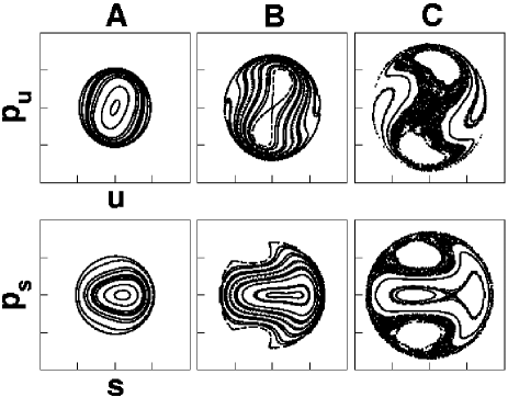
Figure 5: Poincaré surface of sections for the Davis-Heller Hamiltonian. The top panel shows the $(u,p_{u})$ section and the bottom panel shows the $(s,p_{s})$ surface of section for increasing total energy $E=$ 5.0 (A), 9.0 (B), and 14.0 (C). Note that the symmetric stretch periodic orbit ($u=p_{u}=0$) becomes unstable around $E\approx 6.5$ whereas the asymmetric stretch periodic orbit ($s=p_{s}=0$) becomes unstable around $E\approx 8.5$.

The observation by Davis and Heller, implicily present in the work by Lawton and Child, regarding the importance of the $1$:$1$ resonance to the dynamical tunneling was put to test in an elegant series of paperssrh82c ; srh82q by Sibert, Reinhardt, and Hynes. These authors investigated in great detail the classicalsrh82c and quantum dynamicssrh82q of energy transfer between bonds in ABA type triatomics and gave explicit expressions for the splittings. In particular they studied the model H₂O Hamiltonian:

$$H({\bf x},{\bf p})=\sum_{j=1,2}\left(\frac{1}{2}G_{jj}p_{j}^{2}+U(x_{j})\right)+G_{12}p_{1}p_{2}$$ (13)

with $(x_{1},x_{2})$ and $(p_{1},p_{2})$ denoting the two OH bond stretches (local modes) and their corresponding momenta respectively. The bending motion was ignored and the stretches were modelled by Morse oscillators

$$U(x)=D\left[1-e^{-ax}\right]^{2}$$ (14)

with $D$ being the OH bond dissociation energy. Due to the equivalence of the OH stretches $G_{11}=G_{22}$ and the coupling strength $G_{12}$ is much smaller than $G_{11}$. The authors studied the dynamics of initial states $|n_{1},n_{2}\rangle$ where $|n_{j}\rangle$ are eigenstates of the unperturbed j^th Morse oscillator. Due to the coupling the initial states have nontrivial dynamics and thus mix with other zeroth-order states. An initial state $|n_{1},n_{2}\rangle$ implies a certain energy distribution in the molecule and the nontrivial time dependence signals flow of energy in the molecule. Later studies by Hutchinson, Sibert, and Hynes showedhsh84 that based on the dynamics the various initial states could be classified as normal modes or local modes. Morever at the border between the two classes were initial states that led to a ‘nonclassical’ energy flow. A representative example, using a different but equivalent system, for the three classes is shown in Fig. 6. The normal mode regime illustrated with $|n_{1},n_{2}\rangle=|3,2\rangle$ shows complete energy flow between the modes on the time scale of a few vibrational periods - something that occurs classically as well. The local mode behaviour for the initial state $|3,0\rangle$ exhibits complete energy transfer resulting in the state $|0,3\rangle$ but the timescale is now hundreds of vibrational periods. Despite the large timescales involved it is important to note that such a process does not happen classically. Thus this is an example of dynamical tunneling. The so called nonclassical case illustrated with an initial state $|3,1\rangle$ is also an example of dynamical tunneling. However the associated timescale is nowhere as large when compared to the local mode regimehsh84 .

The vibrational energy transfer process illustrated through the initial state $|3,0\rangle$ and $|3,1\rangle$ are examples of pure quantum routes to energy flow. Hutchinson, Sibert, and Hynes proposedhsh84 that the mechanism for this quantum energy flow can be understood as an indirect state-to-state flow of probability involving normal mode intermediate states. For instance, in the case involving the initial state $|3,0\rangle$ the following mechanism was proposed:

$$|3,0\rangle\rightarrow|2,1\rangle\rightarrow|1,2\rangle\rightarrow|0,3\rangle$$ (15)

The reason for this indirect route has to do with the fact that estimating the splitting directly (at first order) $\Delta=2\langle 3,0|G_{12}p_{1}p_{2}|0,3\rangle$ yields a value which is more than an order of magnitude smaller than the the actual valuehsh84 . Indeed note that the indirect route corresponds to a third order perturbation in the coupling and hence it is possible to estimate the contribution to the splitting as:

$$\frac{\Delta}{2}=\frac{\langle 3,0|V|2,1\rangle\langle 2,1|V|1,2\rangle\langle 1,2|V|0,3\rangle}{(E^{0}_{3,0}-E^{0}_{2,1})^{2}}$$ (16)

with $V\equiv G_{12}p_{1}p_{2}$ and $E^{0}_{n_{1},n_{2}}$ are the zeroth-order energies associated with the states $|n_{1},n_{2}\rangle$.

Once again a clear interpretation of the mechanism comes from taking a closer look at the underlying classical phase spacesrh82c ; hsh84 . Using the classical action-angle variables $({\bf I},{\bm{\theta}})$ for Morse oscillators it is possible to write the original Hamiltonian in Eq. (13) as:

$$H({\bf I},{\bm{\theta}})=\sum_{i=1,2}\left(\Omega I_{i}-\frac{\Omega^{2}I_{i}^{2}}{4D}\right)+V({\bf I},{\bm{\theta}})$$ (17)

with the harmonic frequency $\Omega=\sqrt{2DG_{11}a^{2}}$. The coupling term $V({\bf I},{\bm{\theta}})$ has infinitely many terms of the form $V_{pq}({\bf I})\cos(p\theta_{1}-q\theta_{2})$ which represent nonlinear resonances $p\omega_{1}\approx q\omega_{2}$ involving the nonlinear mode frequencies $\omega_{i}=\Omega-\Omega^{2}I_{i}/2D$. Arguments were providedsrh82c for the dominance of the $p=q=1$ resonance and hence to an excellent approximation

$$H({\bf I},{\bm{\theta}}) \approx \sum_{i=1,2}\left(\Omega I_{i}-\frac{\Omega^{2}I_{i}^{2}}{4D}\right)+V_{11}({\bf I})\cos(\theta_{1}-\theta_{2})$$ (18)

$$\approx \Omega P-\frac{\Omega^{2}P^{2}}{8D}-\left(\frac{\Omega^{2}p^{2}}{8D}+V_{0}(P,p)\cos(2\psi)\right)$$

$$\equiv H_{M}(P)-H_{R}(p,\psi)$$

The form $H_{M}-H_{R}$ originates via a canonical transformation from $({\bf I},{\bm{\theta}})\rightarrow(P,\phi,p,\psi)$ with $I_{1}+I_{2}=P$,$I_{1}-I_{2}=p$,$\theta_{1}+\theta_{2}=2\phi$, and $\theta_{1}-\theta_{2}=2\psi$. Thus the key term in the above Hamiltonian is the hindered rotor part denoted by $H_{R}(p,\psi)$ and the analysis now focuses on a one dimensional Hamiltonian due to the fact that $P$ is a conserved quantity. Note that this is consistent with the observationlc81 by Lawton and Child regarding the evaluation of the frequency factor $\hbar\bar{\omega}_{nm}$ in eq. 11. The classical variables $(P,p)$ are quantized as $P=(n_{1}+n_{2}+1)\hbar\equiv(m+1)\hbar$ and $p=(n_{1}-n_{2})\hbar\equiv r\hbar$;thereby the rotor barrier is different for different states $|m,r\rangle$ i.e., $V_{0}=V_{0}(m,r)$. In this rotor representation, motion below and above the rotor barrier correspond to normal and local mode behaviour respectively. Exploiting the fact that $H_{R}$ is a one dimensional Hamiltonian a semiclassical (WKB) expression for the local mode splitting can be written down as

$$\frac{\Delta}{2}=\frac{\omega_{0}}{2\pi}e^{-\theta}$$ (19)

The frequency factor is $\omega_{0}=2\partial H_{R}/\partial p$ and the the tunneling action integral $\theta$ is taken between the two turning points $p(\psi*)=0$. Since the local modes are above the rotor barrier the turning points are purely imaginary $\psi*\equiv i\eta*=\cosh^{-1}(E^{0}_{R}/V_{0})/2$ and thus

$$\theta\equiv\int d\psi p(\psi)=\int_{-\eta*}^{\eta*}d\eta\sqrt{8D(E^{0}_{R}-V_{0}\cosh(2\eta))}$$ (20)

where, $E^{0}_{R}=\Omega^{2}r^{2}/8D$ and a crucial assumption has been made that $V_{0}$ does not depend on $p$. Although such an asusmption is not strictly valid the estimates for the splittings agreed fairly well with the exact quantum values.

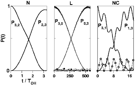
Figure 6: Three classes of energy flow dynamics, normal (N), local (L), and nonclassical (NC) illustrated for the coupled Morse system by computing the survival probabilities $P(t)$ for the states $|3,2\rangle$, $|3,0\rangle$, and $|3,1\rangle$ respectively. The cases L and NC are examples of dynamical tunneling whereas case N occurs classically. Note the difference in the timescales for complete energy transfer between modes for L and NC. In the case of NC significant probability builds up in the normal mode state $|2,2\rangle$ (symbols). Very little probability buildup in the intermediate states $|2,1\rangle$ (open circles) and $|1,2\rangle$ (filled circles) is seen in case L.

The analysis thus implicates a $\omega_{1}$:$\omega_{2}=1$:$1$ nonlinear resonance in the phase space for the dynamical tunneling between local modes and several interesting observations were made. First, the rotor Hamiltonian explains the coupling scheme outlined in Eq. (15). Second, although there is a fairly strong coupling between $|3,0\rangle$ and the intermediate state $|2,1\rangle$ no substantial probability build-up was noticed in the state $|2,1\rangle$ (cf. Fig. 6L). On the other hand substantial probability does accumulate, as shown in Fig. 6 (NC), in the intermediate state $|2,2\rangle$ involved in the energy transfer process $|3,1\rangle\leftrightarrow|1,3\rangle$. It was also commentedhsh84 that the double well analogy provided by Davis and Hellerdh81 ; dh84 was very different from the one that emerges from the hindered rotor analysis - local modes in the former case would be trapped below the barrier whereas they are above the barrier in the latter case. Finally, a very important observationhsh84 was that small amounts of asymmetry between the two modes quenched the $|3,0\rangle\leftrightarrow|0,3\rangle$ process whereas there was little effect on the $|3,1\rangle\leftrightarrow|1,3\rangle$ process. The different effects of the asymmetry was one of the primary reasons for distinguishing between local and nonclassical states.

Several questions arise at this stage. Is the rotor analysis applicable to the Lawton-Child and Davis-Heller systems? Why is there a difference in the interpretation of the local modes, and hence the mechanism of dynamical tunneling, between the phase space and hindered rotor pictures? Is it reasonable to neglect the higher order $\omega_{1}$:$\omega_{2}=p$:$q$ resonances solely based on the relative strengths? If multiple resonances do exist then one has the possibility of their overlap leading to chaos. Is it still possible to use the rotor formalism in the mixed phase space regimes? Some of the questions were answered in a work by Stefanski and Pollak wherein a periodic orbit quantization technique was proposed to calculate the splittingssp87 . Stefanski and Pollak pointed outsp87 an important difference between the Davis-Heller and the Sibert-Reinhardt-Hynes Hamiltonians in terms of the periodic orbits at low energies. Nevertheless, they were able to show that a harmonic approximation to the tunneling action integral Eq. (20) yields an expression for the splitting which is identical to the one derived by assuming that the symmetric stretch periodic (unstable) orbit gives rise to a barrier separating the two local mode states - an interpretation that Davis and Heller provided in their workdh81 . Thus Stefanski and Pollak resolved an apparent paradox and emphasized the true phase space nature of dynamical tunneling.

In any case it is worth noting that irrespective of the representation the key feature is the existence of a dynamical barrier separating two qualitatively different motions; the corresponding structure in the phase space had to do with the appearance of a resonance. Further support for the importance of the resonance to tunneling between tori in the phase space came from a beautiful analysis by Ozorio de AlmeidaOzo84 which, as seen later, forms an important basis for the recent advances. A different viewpoint, using group theoretic arguments, based on the concept of dynamical symmetry breaking was advancedKell82 by Kellman. Adapting Kellman’s arguments, originally applied to the local mode spectrum of benzene, imagine placing one quantum in one of the local O-H stretching mode of H₂O. Classially the energy remains localized in this bond and thus there is a lowering or breaking of the $C_{2v}$ point group symmetry of the molecule. However quantum mechanically, dynamical tunneling restores the broken symmetry. Invoking the more general permutation-inversion groupbunkjenbook and its feasible subgroups provides insights into the pattern of local mode splittings and hence insights into the energy transfer pathways via dynamical tunneling. The dominance of a pathway of course cannot be established within a group theoretic approach alone and requires additional analysis. Note that recentlybwf03 Babyuk, Wyatt, and Frederick have reexamined the dynamical tunneling in the Davis-Heller and the coupled Morse systems via the Bohmian approach to quantum mechanics. Analysing the relevant quantum trajectories Babyuk et al. discovered that there were several regions, at different times, wherein the potential energy exceeds the total energy (which includes the quantum potential). In this sense, locally, one has a picture that is similar to tunneling through a one dimensional potential barrier. Interestingly such regions were associated with the so-called quasinodes which arise during the dynamical evolution of the density. Therefore the dynamical nature of the barriers is clearly evident, but more work is needed to understand the origin and distributions of the quasinodes in a given system. Needless to say, correlating the nature of the quasinodes to the underlying phase space structures would be a useful endeavour.

III Quantum mechanism: vibrational superexchange

The earlier works established the importance of the phase space perspective for dynamical tunneling using systems that possesed discrete symmetries and therefore implicitly invoked an analogy to symmetric double well models. That is not to say that the earlier studies presumed that dynamical tunneling would only occur in symmetric systems. Indeed a careful study of the various papers reveal several insightful comments on asymmetric systems as well. However mechanistic details and quantitative estimates for dynamical tunneling rates were lacking. Important contributions in this regard were made by Stuchebrukhov, Mehta, and Marcus nearly a decade agosm93 ; sm932 ; smm93 ; msm95 . The experimentsklmps91 that motivated these studies have been discussed earlier in the introduction. In this section the key aspects of the mechanism are highlighted.

The inspiration comes from the well known superexchange mechanism of long distance electron transfer in moleculesNew91 ; sm92 . Stuchebrukhov and Marcus arguedsm93 ; sm932 that since the initial, localized (bright) state is not directly coupled by anharmonic resonances to the other zeroth-order states it is necessary to invoke off-resonant virtual states to explain the sluggish flow of energy. Specifically, it was noted that at any given time very little probability accumulates in the virtual states. In this sense the situation is very similar to the mechanism proposed by Hutchinson, Sibert, and Hyneshsh84 as illustrated by Eq. (15). However Stuchebrukhov and Marcus extended the mechanism, called as vibrational superexchangesm932 , to explain the flow of energy between inequivalent bonds in the molecule and noted the surprising accuracy despite the large number of virtual transitions involved in the process. As noted earlier, Hutchinson’s workHut84 on state mixing in cyanoacetylene also illustrated the flow of energy between inequivalent modes. In order to illustrate the essential idea consider the hindered rotor Hamiltonian (cf. Eq. (18)):

$$H_{R}=\frac{p^{2}}{2I}+V_{0}(P,p)\cos(2\psi)$$ (21)

where we have denoted $I\equiv 4D/\Omega^{2}$. The free rotor energies and the associated eigenstates are known to be

$$E_{R}^{0}(k) = \frac{k^{2}}{2I}$$ (22a)

$$\langle\psi|k\rangle = \frac{1}{\sqrt{2\pi}}\exp(ik\psi)$$ (22b)

The perturbation to the free rotor connects states that differ by two rotational quanta i.e., $\langle k|V_{0}(P,p)\cos(2\psi)|k^{\prime}\rangle\approx V_{0}(P)/2$ with $|k-k^{\prime}|=2$. Clearly the local mode states $|m,r\rangle$, and $|m,-r\rangle$ with $r\gg 1$ are not directly connected by the perturbation. Nevertheless the local mode states can be coupled through a sequence of intermediate virtual states with quantum numbers $-(r-2)\leq k\leq(r-2)$. The effective coupling matrix element

$$V_{\rm eff}=\frac{V_{0}}{2}\prod_{l=-(r-2)}^{(r-2)}\frac{V_{0}/2}{E_{R}^{0}(r)-E_{R}^{0}(l)}$$ (23)

can be obtained via a standard application of high-order perturbation theory involving the sequence

$$|m,r\rangle\rightarrow|m,r-2\rangle\rightarrow\ldots\rightarrow|m,-(r-2)\rangle\rightarrow|m,-r\rangle$$ (24)

Note that the polyad quantum number $m$ in the above sequence is fixed and is consistent with the single resonance approximation. In addition $V_{0}/2\ll E_{R}(r)-E_{R}(r-2)$ must be satisfied for the perturbation theory to be valid. Thus the splitting between the symmetry related local mode states $|m,\pm r\rangle$ is given by $\Delta_{m,r}=2V_{\rm eff}$. Interestingly, Stuchebrukhov and Marcus showedsm932 that $V_{\rm eff}$ could be derived by analysing the semiclassical action integral

$$\theta=\int_{-p_{m}}^{p_{m}}dp\,\eta(p)$$ (25)

with $\eta=-i\psi$ and $|p_{m}|=\sqrt{2I(E_{R}^{0}(r)-V_{0})}$ being the minimum classical value of the momentum of the rotor excited above the barrier $V_{0}$. This suggests that the high-order perturbation theory, if valid, is the correct approach to calculating dynamical tunneling splittings in multidimensions. An additional consequence is that the nonclassical mechanism of IVR is equivalent to dynamical tunneling as opposed to the earlier suggestionhsh84 of an activated barrier crossing. As a cautionary note it must be mentioned that the above statements are based on insights afforded by near-integrable classical dynamics with two degrees of freedom.

Although the example above corresponds to a symmetric case the arguments are fairly general. In fact the vibrational superexchange mechanism is appropriate for describing quantum pathways for IVR in molecules. For example consider the acetylinic CH-stretch ($\nu_{1}$) excitations in propyne, H₃CCCH. Experiments by Lehmann, Scoles, and coworkersgtls93 indicate that the overtone state $3\nu_{1}$ has a faster IVR rate as compared to the nearly degenerate $\nu_{1}+2\nu_{6}$ combination state. Similarly Go, Cronin, and Perry in their studygcp93 found evidence for a larger number of perturbers for the $2\nu_{1}$ state than for the $\nu_{1}+\nu_{6}$ state. The spectrum corresponding to both the first and the second overtone states implied a lack of direct low-order Fermi resonances. It was shownmsm95 that the slow IVR out of the $2\nu_{1}$ and $3\nu_{1}$ states of propyne can be explained and understood via the vibrational superexchange mechanism.

There is little doubt that the vibrational superexchange mechanism, as long as one is within the perturbative regimes, is applicable to fairly large molecules. However several issues still remain unclear. The main issue has to do with the effective coupling between the initial bright state $|{\bf b}\rangle\equiv|v_{1}^{b},v_{2}^{b},\ldots\rangle$ and a nearly degenerate zeroth-order dark state $|{\bf d}\rangle\equiv|v_{1}^{d},v_{2}^{d},\ldots\rangle$ in the multidimensional state space. In the case of a lone anharmonic resonance there is only a single off-resonant sequence of states connecting $|{\bf b}\rangle$ and $|{\bf d}\rangle$ as in Eq. (24). This sequence or chain of states translates to a path in the state space. Note that the ‘paths’ being refered to here are nondynamical, although it might be possible to provide a dynamical interpretation by analysing appropriate discrete action functionalssm93 . In general there are several anharmonic resonances of different orders and in such instances the number of state space paths can become very large and the issue of the relative importance of one path over the other arises. For instance it could very well be the case that $|{\bf b}\rangle$ and $|{\bf d}\rangle$ can be connected by a path with many steps involving low order resonances and also by a path involving few steps using higher order resonances. It is not a priori clear as to which path should be considered. An obvious choice is to use some perturbative criteria to decide between the many paths. Such a procedure was used by Stuchebrukhov and Marcus to create the tiers in their analysissm93 . More recentlypg98 Pearman and Gruebele have used the perturbative criteria to estimate the importance of direct high/low order couplings and low order coupling chains to the IVR dynamics in the state space. Thus consider the following possible coupling chains, shown in Fig. 3, assuming that the states $|{\bf b}\rangle$ and $|{\bf d}\rangle$ are separated by $n$ quanta in the state space i.e., $\sum|v_{k}^{b}-v_{k}^{d}|=n$

$$|{\bf b}\rangle \stackrel{{\scriptstyle n}}{{\longrightarrow}} |{\bf d}\rangle$$

$$|{\bf b}\rangle \stackrel{{\scriptstyle n_{1}}}{{\longrightarrow}} |{\bf i}_{1}\rangle\stackrel{{\scriptstyle n_{2}}}{{\longrightarrow}}|{\bf d}\rangle$$

$$|{\bf b}\rangle \stackrel{{\scriptstyle n_{1}}}{{\longrightarrow}} |{\bf i}_{1}\rangle\stackrel{{\scriptstyle n_{2}}}{{\longrightarrow}}|{\bf i}_{2}\rangle\stackrel{{\scriptstyle n_{3}}}{{\longrightarrow}}|{\bf d}\rangle$$

Note that $n$ is the distance between $|{\bf b}\rangle$ and $|{\bf d}\rangle$ in the state space and thus identical to $Q$ in Eq. (10). In the above the first equation indicates a direct coupling between the states of interest by an anharmonic resonance coupling $V_{bd}^{(n)}$ of order $n$. In the second case the coupling is mediated by one intermediate state $|{\bf i}_{1}\rangle$ involving two anharmonic resonances $V_{bi_{1}}^{(n_{1})}$ and $V_{i_{1}d}^{(n_{2})}$ with $n=n_{1}+n_{2}$. Each step of a given state space path, coupling two states $|{\bf i}\rangle$ and $|{\bf j}\rangle$ at order $m$, is weighted by the perturbative term

$${\cal L}_{ij}^{(m)} = \left\{1+\left(\frac{\Delta E_{ij}^{0}}{V_{ij}^{(m)}}\right)^{2}\right\}^{-1/2}$$

$$\approx \frac{V_{ij}^{(m)}}{\Delta E_{ij}^{0}}\qquad{\rm for}\quad\Delta E_{ij}^{0}\gg V_{ij}^{(m)}$$

$$\approx 1\qquad\qquad{\rm for}\quad\Delta E_{ij}^{0}\ll V_{ij}^{(m)}$$

with $\Delta E_{ij}^{0}\equiv E_{i}^{0}-E_{j}^{0}$ and $V_{ij}^{(m)}\equiv\langle{\bf i}|V^{(m)}|{\bf j}\rangle$. A specific path in the state space is then associated with the product of the weightings for each step along the path. For example the state space path above involving two intermediate states is associated with the term ${\cal L}_{bi_{1}}^{(n_{1})}{\cal L}_{i_{1}i_{2}}^{(n_{2})}{\cal L}_{i_{2}d}^{(n_{3})}$. It is not hard to see that such products of ${\cal L}$ correspond to the terms contributing to the effective coupling as shown in Eq. (16) and Eq. (23). The various terms also contribute to the effective coupling $\psi_{Q}$ (cf. Eq. (10)) in the Leitner-Wolynes criterialw96jcp for the transition from localized to extended states.

The crucial issue is wether or not one can identify dominant paths, equivalently the key intermediate states, based on the perturbative criteria alone. In a rigorous sense the answer is negative since such a criteria ignores the dynamics. Complications can also arise due to the fact that each segment of the path contributes with a $\pm$ phasepg98 . Furthermore one would like to construct the explicit dynamical barriers in terms of the molecular parameters and conserved or quasi-conserved quantities. The observation that the superexchange $V_{\rm eff}$ can be derivedsm93 from a semiclassical action integral provides a clue to some of the issues. However an explicit demonstration of such a correspondence has been provided only in the single resonance (hindered rotor) case. In the multidimensional case the multiplicity of paths obscures this correspondence. The next few sections highlight the recent advances which show that clear answers to the various questions raised above come from viewing the phenomenon of dynamical tunneling in the most natural representation - the classical phase space.

IV Dynamical tunneling: recent work

Nearly a decade ago Heller wrote a brief reviewHel95 on dynamical tunneling and its spectral consequences which was motivated in large part by the work of Stuchebrukhov and Marcussm93 . Focusing on systems with two degrees of freedom in the near-integrable regimes, characteristic of polyatomic molecules at low energies, Heller argued that the $10^{-1}$-$10^{-2}$ cm^-1 broadening of lines is due to dynamical tunneling between remote regions of phase space facilitated by distant resonances. This is an intriguing statement which could perhaps be interpreted in many different ways. Moreover the meaning of the words ’remote’ and ’distant’ are not immediately clear and fraught with conceptual difficulties in a multidimensional phase space setting. In essence Heller’s statement, more appropriately called as a conjecture, is an effort to provide a phase space picture of the superexchange mixing between two or more widely separated zeroth-order states in the state space. Some of the examples in the later part of the present review, hopefully, demonstrate that the conjecture is reasonable. Interestingly though in the same review it is mentionedHel95 that in the presence of widespread chaos the issue of tunneling as a mechanism for IVR is of doubtful utility. Similar sentiments were echoed by Stuchebrukhov et al. who, in the case of high dimensional phase spaces, envisaged partial rupturing of the invariant tori and hence domination of IVR by chaotic diffusion rather than dynamical tunneling. This too has to be considered as a conjecture at the present time since the timescales and the competition between chaotic diffusion (classically allowed) and dynamical tunneling (classically forbidden) in systems with three or more degrees of freedom has not been studied in any detail. The issues involved are subtle and extrapolating the insights from studies on two degrees of freedom to higher degrees of freedom is incorrect. For instance, in three and higher degrees of freedom the invariant tori, ruptured or not, do not have the right dimensionality to act as barriers to inhibit diffusion. Therefore, is it possible that classical chaos could assist or inhibit dynamical tunneling? Several studieslb91r ; si95 ; bbem93 ; btu93 ; tu94 ; lgw94 ; ammk95 ; udh94 ; df95 ; lu96 ; si96 carried out during the early nineties till the present time point to an important role played by chaos in the process of dynamical tunneling. We start with a brief review of these studies followed by very detailed investigations into the role played by the nonlinear resonances. Finally, some of the very recent work is highlighted which suggest that the combination of resonances and chaos in the phase space can yet play an important role in IVR.

IV.1 Chaos-assisted tunneling (CAT)

One of the first studies on the possible influence of chaos on tunneling was made by Lin and Ballentinelb90 ; lb91r ; lb92 . These authors investigated the tunneling dynamics of a driven double well system described by the Hamiltonian

$$H(x,p,t)=\frac{1}{2m}p^{2}+bx^{4}-dx^{2}+\lambda_{1}x\cos(\omega t)$$ (27)

which has the discrete symmetry $H(x,p,t)=H(-x,-p,t+T_{0}/2)$ with $T_{0}=2\pi/\omega$. In the absence of the monochromatic field ($\lambda_{1}=0$) the system is integrable and the phase space is identical to that of a one dimensional symmetric double well potential. However with $\lambda_{1}\neq 0$ the system is nonintegrable and the phase space is mixed regular-chaotic. Despite the mixed phase space the discrete symmetry implies that any regular islands in the phase space will occur in symmetry related pairs and the quantum floquet states will occur as doublets with even/odd symmetries. A coherent state (wavepacket) localized on one of the regular islands will tunnel to the other, clasically disconnected, symmetry related island. Thus this is an example of dynamical tunneling. An important observation by Lin and Ballentine was that the tunneling was enhancedlb90 ; lb92 by orders of magnitude in regimes wherein significant chaos existed in the phase space. For example with $\lambda_{1}=0$ the ground state tunneling time is about $10^{6}T_{0}$ whereas with $\lambda_{1}=10$ the tunneling time is only about $10^{2}T_{0}$. Futhermore strong fluctuations in the tunneling times were observed. In Fig. 7 a typical example of the fluctuations over several orders of magnitude are shown. The crucial thing to note, however, is that the gross phase space structures are similar over the entire range shown in Fig. 7. Thus although the chaos seems to influence the tunneling the mechanistic insights were lacking i.e., the precise role of the stochasticity was not understood.

Figure 7: Tunneling time for the Lin-Ballentine system as a function of the field strength $\lambda_{1}$. The parameters are chosenlb90 as $m=1$, $b=0.5$, and $d=10$. The phase space for $\lambda_{1}=7.8$ in the upper left panel shows the two regular islands embedded in the chaotic sea. The initial state corresponds to a coherent state localized on the left regular island (indicated by an arrow). The three phase space strobe plots at increasing values of $\lambda_{1}$ indicated in (a) show the local structure near the left island. Despite the phase space being very similar the tunneling times fluctuate over many orders of magnitude. Figure courtesy of Astha Sethi (unpublished work).

Important insights came from the workgdjh91 by Grossmann et al. who showed that it is possible to suppress the tunneling in the driven double well by an appropriate choice of the field parameters $(\lambda_{1},\omega)$. The explanantion for such a coherent destruction of tunneling and the fluctuations comes from analysing the the floquet level motions with $\lambda_{1}$. Gomez Llorente and Plata providedlp92 perturbative estimates within a two-level approximation for the enhancement/suppression of tunneling. A little later Utermann, Dittrich, and Hänggi showedudh94 that there is a strong correlation between the splittings of the floquet states and their overlaps with the chaotic part of the phase space. Breuer and Holthausbh93 highlighted the role of classical phase space structures in the driven double well system. Subsequently other worksfm93 ; lgw94 ; ammk95 ; fh96 ; zl97 ; mmkgd01 ; om05 on a wide variety of driven systems established the sensitivity of tunneling to the classical stochasticity. An early discussion of dynamical tunneling and the influence of dissipation can be found in the workgh87 by Grobe and Haake on kicked tops. A comprehensive account of the various studies on driven systems can be found in the reviewgh98 by Grifoni and Hänggi. Such studies have provided, in recent times, important insights into the process of coherent control of quantum processes. Recent reviewgb05 by Gong and Brumer, for instance, discusses the issue of quantum control of classically chaotic systems in detail. Perhaps it is apt to highlight a historical fact mentioned by Gong and Brumer - coherent control emerged from two research groups engaged in studies of chaotic dynamics.

In the Lin-Ballentine example above the perturbation (applied field) not only increases the size of the chaotic region but also affects the dynamics of the unperturbed tunneling doublet. Hence the enhanced tunneling, relative to the unperturbed or the weakly perturbed case, cannot be immediately ascribed to the increased amount of chaos in the phase space. To observe a more direct influence of chaos on tunneling it is necessary that the classical phase space dynamics scales with energy. Investigations of the coupled quartic oscillator system by Bohigas, Tomsovic, and Ullmobtu93 ; tu94 provided the first detailed view of the CAT process. The choice of the Hamiltonian

$$H({\bf p},{\bf q})=\frac{1}{2}{\bf p}^{2}+a(\lambda)\left[\frac{q_{1}^{4}}{b}+bq_{2}^{4}+2\lambda q_{1}^{2}q_{2}^{2}\right]$$ (28)

with $b=\pi/4$ was made in order to study the classical-quantum correspondence in detail. This is due to the fact that the potential is homogeneous and hence the dynamics at a specific energy $E$ is related to the dynamics at a different energy by a simple rescaling. Consequently one can fix the energy and investigate the effect of the semiclassical limit $\hbar\rightarrow 0$ on the tunneling process. The classical dynamics is integrable for $\lambda=0$ and strongly chaotic for $\lambda=-1$. Again, note that the Hamiltonian has the discrete symmetry ${\bf q}\rightarrow-{\bf q},{\bf p}\rightarrow-{\bf p}$ and thus the quantum eigenstates are expected to show up as symmetry doublets. In contrast to the driven system discussed above, and similar to the Davis-Heller system discussed earlier, the system in eq. (28) does not have any barriers arising from the two dimensional quartic potential. The doublets therefore must correspond to quantum states localized in the symmetry related islands in phase space shown in Fig. 8. Thus denoting the states localized in the top and bottom regular islands by $|T\rangle$ and $|B\rangle$ respectively the doublets correspond to the usual linear combinations $|\pm\rangle=(|T\rangle\pm|B\rangle)/\sqrt{2}$.

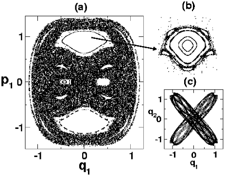
Figure 8: In (a) the $q_{2}=0$ surface of section is shown for $E=1$ and the parameter values $(\lambda,b)=(-0.25,\pi/4)$ for the Hamiltonian in Eq. (28). The large islands are part of a $1$:$1$ resonance island chain and are related to each other by symmetry. (b) Details of the upper island and (c) shows the configuration space plot of the symmetrically related tori.

Bohigas, Tomsovic, and Ullmo focused on quantum states associated with the large regular islands seen in Fig. 8. Specifically, they studied the variations in the splitting $\Delta E\equiv|E_{+}-E_{-}|$ associated with the doublets $|\pm\rangle$ upon changing $\hbar$ and the coupling $\lambda$. Since the states are residing in a regular region of the phase space it is expected, based on one dimensional tunneling theories, that the splittings will scale exponentially with $\hbar$ i.e., $\Delta E\sim\exp(-1/\hbar)$. However the splittings exhibitbtu93 fluctuations of several orders of magnitude and no obvious indication of a predictable dependence on $\hbar$ seemed to exist. Note that a similar feature is seen in Fig. 7 showing the tunneling time fluctuations of the driven double well system. More precisely, it was observedbtu93 that for the range of $\lambda$ that corresponded to integrable or near-integrable phase space $\Delta E$ roughly follows the exponential scaling. On the other hand for $\lambda=\lambda^{*}\approx-0.2$ chaos becomes pervasive and $\Delta E$ exhibits severe fluctuations. Tomsovic and Ullmo arguedtu94 that the fluctuations in $\Delta E$ could be traced to the crossing of the quasidegenerate doublets with a third irregular state. By irregular it is meant that when viewed from the phase space the state density, represented by either the Wigner or the Husimi distribution function, is appreciable in the chaotic sea. The irregular state, in contrast to the regular states, do not come as doublets since there is no dynamical partition of the chaotic region into mutually exclusive symmetric parts. Nevertheless the irregular states do have fixed parities with respect to the reflection operations. Thus chaos-assisted tunneling is necessarily atleast a three-state processtu94 ; bbem93 . In other words, assuming that the even-parity irregular state $|C\rangle$ with energy $E_{c}$ couples to $|+\rangle$ with strength $v$ a relevant, but minimal, model Hamiltonian in the symmetrized basis has the form:

$$H=\left(\begin{array}[]{ccc}E+\epsilon&0&0\\ 0&E-\epsilon&v\\ 0&v&E_{c}\end{array}\right)$$ (29)

with $\epsilon$ being a direct coupling between $|T\rangle$ and $|B\rangle$. If $\epsilon$ is dominant as compared to $v$ then one has the usual two level scenario. However if $v\gg\epsilon\approx 0$ then the splitting can be approximated as

$$\Delta E\rightarrow\begin{cases}\frac{v^{2}}{E-E_{c}}&E-E_{c}\gg v,\\ |v|&E-E_{c}\ll v.\end{cases}$$ (30)

Hence varying a parameter, for example $\lambda$, one expects a peak of height $|v|$ as $E_{c}$ crosses the $E_{+}$ level. Detailed theoretical studiesdf95 ; df98 of the dynamical tunneling process in annular billiards by Frischat and Doron confirmed the crucial role of the classical phase space structure. Specifically it was found that the tunneling between two symmetry related whisphering gallery modes (corresponding to clockwise and counterclockwise rotating motion in the billiard) is strongly influenced by quantum states that inhabit the regular-chaotic border in the phase space. Such states were termed as “beach states” by Frischat and Doron. Soon thereafter Dembowski et al. provided experimental evidencedghhrr00 for CAT in a microwave annular billiard simulated by means of a two-dimensional electromagnetic microwave resonator. Details of the experiment can be found in a recent paperhadghhrr05 by Hofferbert et al. wherein support for the crucial role of the beach region is provided. It is, however, significant to note that the regular-chaotic border in case of the annular billiards is quite sharp.

An important point to note is that despite the intutively appealing three-state model, determining the coupling $v$ between the regular and chaotic states is nontrivial. This, in turn, is related to the fact that accurate determination of the positions of the chaotic levels can be a difficult task and determining the nature of a chaotic state for systems with mixed phase spaces is still an open problem. Such difficulties prompted Tomsovic and Ullmotu94 to adopt a statistical approach, based on random matrix theory, to determine the tunneling splitting distribution $P(\Delta E)$ in terms of the variance of the regular-chaotic coupling i.e., $\overline{v^{2}}$. In a later work Leyvraz and Ullmo showedlu96 that $P(\Delta E)$ is a truncated Cauchy distribution

$$P(\Delta E)=\frac{2}{\pi}\frac{\overline{\Delta E}}{(\Delta E)^{2}+(\overline{\Delta E})^{2}}$$ (31)

with $\overline{\Delta E}$ being the mean splitting. On the other hand Creagh and Whelancw00 ; cw99 showed that the splitting between states localized in the chaotic regions of the phase space but separated by an energetic barrier is characterized by a specific tunneling orbit. Specifically, the resulting splitting distribution depends on the stability of the tunneling orbit and is not universal. In certain limitscw00 the splittings obey the Porter-Thomas distribution. Thus the fluctuations in $\Delta E$ in the CAT process are different from those found in the usual double-well system. Note that in case of CAT the distribution pertains to the splitting between states localized in the regular regions of phase space embedded in the chaotic sea. The reader is referred to the excellent discussion by Creagh for detailsCrebook . Nevertheless, in a recent work Mouchet and Delande observedmd03 that the $P(\Delta E)$ exhibits a truncated Cauchy behaviour despite a near-integrable phase space. Similar observations have been made by Carvalho and Mijolaro in their study of the splitting distribution in the annular billiard system as wellcm04 . This indicates that the Leyvraz-Ullmo distribution Eq. (31) is not sufficient to characterize CAT. A first step towards obtaining a semiclassical estimate of the regular-chaotic coupling was taken by Podolskiy and Narimanovpn03 . Assuming a regular island seperated by a structureless, on the scale of $\hbar$, chaotic sea they were able to show that:

$$\Delta E\propto\hbar\frac{\Gamma({\cal A},2{\cal A})}{\Gamma({\cal A}+1,0)}$$ (32)

with ${\cal A}\equiv A/\pi\hbar$ and a system specific proportionality factor which is independent of $\hbar$. The phase space area covered by the regular island is denoted by $A$. Application of the theory by Podolskiy and Narimanov to the splittings between near-degenerate optical modes, localized on a pair of symmetric regular islands in phase space, in a non-integrable microcavity yielded very good agreement with the exact datapn03 . In fact Podolskiy and Narimanov have recently shownpn05 that the lifetimes and emission patterns of optical modes in asymmetric microresonators are strongly affected by CAT. Encouraging results were obtained in the case of tunneling in periodically modulated optial lattices as well. However the agreement in the splittings displayed significant deviations in the deep semiclassical regime i.e., large vaues of $\hbar^{-1}$. Interestingly the critical value of $\hbar^{-1}$ beyond which the disagreement occurs correlates with the existence of plateau regions, discussed in the next section (cf. Fig. 11), in the plot of $\log(\Delta E)$ versus $\hbar^{-1}$. Such plateau regions have been noted earlierrbiwg94 by Roncaglia et al. and in several other recent studieses05 ; seu05 ; wseb06 as well.

The qualitative picture that emerged from the numerous studies is that CAT process is a result of competition between classically allowed (mixing or transport in the chaotic sea) and classically forbidden (tunneling or coupling between regular regions and the chaotic sea) dynamics. Despite the significant advancements, the mechanism by which a state localized in the regular island couples to the chaotic sea continued to puzzle the researchers. It might therefore come as a surprise that based on recent studies there is growing evidence that the explanation for the regular-chaotic coupling lies in the nonlinear resonances and partial barriers in the phase space. The work by Podolskiy and Narimanov provides one possible answer but an equally strong clue is hidden in the plateaus that occur in a typical $\log(\Delta E)$ versus $\hbar^{-1}$ plot. It is perhaps reasonable to expect that the theory of Podolskiy and Narimanov is correct when phase space structures like the nonlinear resonances and partial barriers, ignored in the derivation of Eq. (32), in the vicinity of regular-chaotic border regions are much smaller in area as compared to the Planck constant $\hbar$. However, for sufficiently small $\hbar$ the rich hierarchy of structures like nonlinear resonances, partially broken tori, cantori, and even vague tori in the regular-chaotic border region have to be taken into consideration. It is significant to note that Tomsovic and Ullmo had already recognized the importance of accounting for mechanisms which tend to limit classical transporttu94 and proposed generalized random matrix ensembles as a possible approach. There also exist a number of studiesgrr86 ; grracp89 ; khsw00 ; rp88 ; mh00 , involving less than three degrees of freedom, which highlight the nature of the regular-chaotic border and their importance to tunneling between KAM tori.

A different perspective on the influence of chaos on dynamical tunneling came from the detailed investigations by Ikeda and coworkers involving the studysi95 ; si96 ; si98 ; osit01 ; ti03 ; ti05 of semiclassical propagators in the complex phase space. In particular, deep insights into CAT were gained by examining the so called “Laputa chains” which contribute dominantly to the propagator in the presence of chaossi95 ; si96 . For a detailed review the papersi98 by Shudo and Ikeda is highly reccommended. Hashimoto and Takatsukaht98 discuss a situation wherein dynamical tunneling leads to mixing between states localized about unstable fixed points in the phase space. However in this case the transport is energetically as well as dynamically allowed and it is not very clear whether the term ‘tunneling’ is an appropriate choice.

In the following subsections recent progress towards quantitative prediction of the average tunneling rates, and hence the coupling strengths between the regular and chaotic states, are described. The key ingredient to the success of the theory are the nonlinear resonances in the phase space. In fact, depending on the relative size of $\hbar$, one needs to take multiple nonlinear resonances into account for a correct description of dynamical tunneling. If one asociates the $\hbar$ variation with the related density of states in a molecular system then it is tempting to claim that such a mechanism must be the correct semiclassical limit of the Stuchebrukhov-Marcus vibrational superexchange theory. The discussions in the next section indicate that such a claim is indeed reasonable.

IV.2 Resonance-assisted tunneling (RAT)

The early investigations of dynamical tunneling made it clear that nonlinear resonances played an important role in the phenomenon of dynamical tunneling. However in the majority of the studies one had a single resonance of low order dominating the tunneling process and hence an effectively integrable classical dynamics. Very few attempts were made for systems which had multiple resonances and thus capable of exhibiting near-integrable to mixed phase space dynamics. Moreover studying the tunneling process with varying $\hbar$ is necessary to implicate the nonlinear resonances and other phase space structures without ambiguity. Definitive answers in this regard were provided by Brodier, Schlagheck, and Ullmo in their studybsu01 of time-dependent Hamiltonians. In this section we provide a brief outline of their work and refer the reader to some of the recent reviewsbsu02 ; seu05 ; Schl06 which provide details of the theory and applications to several other systems.

In order to highlight the salient features of RAT consider a one degree of freedom system that evolves under a periodic time-dependent Hamiltonian $H(q,p,t)=H(q,p,t+\tau)$. The phase space structure in this case can be easily visualized by constructing the stroboscopic Poincaré section i.e., plotting $(q,p)$ at integer values of the period $t=n\tau$. We are interested in the generic case wherein the phase space exhibits two symmetry-related regular islands that are embedded in the phase space. Typically the phase space has various nonlinear resonances that arise due to frequency commensurability between the external driving field frequency $\omega\equiv 2\pi/\tau$ and the system frequencies. Fig. 9 shows an example of a near-integrable phase space wherein a few resonances are visible. For the moment assume that a prominent $r$:$s$, say the $10$:$1$ resonance in Fig. 9, nonlinear resonance manifests in the phase space. The motion in the vicinity of this $r$:$s$ resonance can be analysed using secular perturbation theory. In order to do this one introduces a time-independent Hamiltonian $H_{0}(q,p)$ that approximately describes the regular motion in the islands. In particular assume that appropriate action-angle variables $(I,\theta)$ can be introduced such that $H_{0}(q,p)\rightarrow H_{0}(I)$ and thus the total Hamiltonian can be expressed as $H(I,\theta,t)=H_{0}(I)+V(I,\theta,t)$. The term $V$ represents a weak perturbation in the center of the island. A $r$:$s$ nonlinear resonance occurs when

$$r\Omega_{r:s}=s\omega_{f}\,\,\,{\rm with}\,\,\,\Omega_{r:s}\equiv\left[\frac{dH_{0}}{dI}\right]_{I=I_{r:s}}$$ (33)

The resonant action is denoted by $I_{r:s}$. Using techniquesllbook from secular perturbation theory one can show that the dynamics in the vicinity of the nonlinear resonance is described by the new Hamiltonianllbook

$${\cal H}(I,\vartheta,t)\approx\frac{(I-I_{r:s})^{2}}{2m_{r:s}}+{\cal V}(I,\vartheta,t)$$ (34)

with ${\cal V}(I,{\cal\vartheta},t)\equiv{\cal V}(I,\vartheta+\Omega_{r:s}t,t)$, and the “effective mass” parameter $m_{r:s}\equiv(d^{2}H_{0}/dI^{2})^{-1}(I_{r:s})$ is related to the anharmonicity of the system. The new angle $\vartheta\equiv\theta-\Omega_{r:s}t$ varies slowly in time near the resonance and hence, according to adiabatic perturbation theory, one can replace ${\cal V}$ by its time average over $r$-periods of the driving field

$$V(I,\vartheta)\equiv\frac{1}{r\tau}\int_{0}^{r\tau}dt{\cal V}(I,\vartheta,t)$$ (35)

Furthermore, writing the perturbation in terms of a Fourier series and neglecting the action dependence of the Fourier coefficients i.e., evaluated at $I=I_{r:s}$ the effective integrable Hamiltonian is obtained as:

$$H_{r:s}(I,\vartheta)=\frac{(I-I_{r:s})^{2}}{2m_{r:s}}+\sum_{k=1}^{\infty}V_{k}(I_{r:s})\cos(kr\vartheta+\phi_{k})$$ (36)

The above effective Hamiltonian couples the zeroth order states $|n\rangle$ and $|n+kr\rangle$ with a matrix element $V_{k}\exp(i\phi_{k})/2$. Here the quantum numbers refer to the zeroth-order KAM tori inside the large regular island. Thus, the eigenstates of $H_{r:s}$ are admixtures of unperturbed states obeying the “selection rule” $|n^{\prime}-n|=kr$ and perturbatively given by

$$|\tilde{n}\rangle = |n\rangle+\sum_{k\neq 0}\frac{v_{k}}{\Delta E_{n+kr}}|n+kr\rangle$$ (37)

$$+ \sum_{k,k^{\prime}\neq 0}\frac{v_{k}v_{k^{\prime}}}{\Delta E_{n+kr}\Delta E_{n+kr+k^{\prime}r}}|n+kr+k^{\prime}r\rangle$$

where $v_{k}\equiv V_{k}\exp(i\phi_{k})$ and $\Delta E_{j}\equiv E_{n}-E_{j}$. Associating the quantized actions $I_{n}\equiv\hbar(n+1/2)$ with states localized in the regular islands the energy difference

$$E_{n}-E_{n^{\prime}}=\frac{1}{2m_{r:s}}(I_{n}-I_{n^{\prime}})(I_{n}+I_{n^{\prime}}-2I_{r:s})$$ (38)

becomes small if $I_{n}+I_{n^{\prime}}\approx 2I_{r:s}$. In other words, the states $|n\rangle$ and $|n^{\prime}\rangle$ are coupled strongly if they straddle the $r$:$s$ resonance symmetrically. Consequently the nonlinear resonance provides an efficient route to couple the ground state with $I_{0}<I_{r:s}$ to a highly excited state with $I_{kr}>I_{r:s}$.

Once again a crucial issue has to do with the the dominant pathways that couple $|n\rangle$ and $|n+kr\rangle$. Clearly the two states can couple in a one-step process via $V_{k}$ or with a $k$-step process via $V_{1}$. The analysis by Brodier et al., realizing the rapid decrease of the Fourier terms $V_{k}$ with $k$, revealsbsu02 that the $k$-step process is dominant in the semiclassical limit $\hbar\rightarrow 0$. Note that within the effective Hamiltonian $H_{r:s}$ one assumes the dominance of a single nonlinear resonance and hence the focus is on the $r$:$s$ resonance and its higher harmonics. Neglecting the Fourier components with $k>1$ and denoting $2V_{r:s}\equiv V_{1}$ one obtains the standard pendulum Hamiltonian

$$H_{eff}(I,\vartheta)=\frac{(I-I_{r:s})^{2}}{2m_{r:s}}+2V_{r:s}\cos(r\vartheta)$$ (39)

For periodically driven systems the floquet states can be obtained by diagonalizing the one-period time evolution operator. The near degenerate floquet states are characterized by the splitting

$$\Delta\phi_{n}=|\phi_{n}^{+}-\phi_{n}^{-}|$$ (40)

between the quasienergies, or eigenphases, of the symmetric and antisymmetric state. Within the perturbation scheme the ground state ($n=0$) splitting is then obtained as

$$\Delta\phi_{0}=\Delta\phi_{0}^{(0)}+\sum_{k}|{\cal A}_{kr}^{(r:s)}|^{2}\Delta\phi_{kr}^{(0)}$$ (41)

with

$${\cal A}_{kr}^{(r:s)}\equiv\langle kr|0\rangle=\prod_{l=1}^{|k|}\frac{V_{r:s}}{E_{0}-E_{lr}}$$ (42)

being a measure of the contribution of the $kr$-th excited state to the perturbed ground state. The quantities $\Delta\phi_{n}^{(0)}$ are the unperturbed splittings resulting from the integrable limit Hamiltonian for which extensive semiclassical insights existWil86 ; sc06 ; tww95 . Note that the above expression for ${\cal A}_{kr}^{(r:s)}$ is essentially the same as the one obtained by Stuchebrukhov and Marcus within their vibrational superexchange approachsm93 . Here one has the generalization for driven systems whose phase space exhibits a general $r$:$s$ nonlinear resonance.

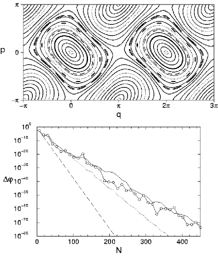
Figure 9: The classical phase space (upper panel) and quantum eigenphase splittings (lower panel) of the kicked Harper system with $\tau=1$. The splittings are calculated for the $n$-th excited state at $N\equiv 2\pi/\hbar=6(2n+1)$. Variation with $N$ is equivalent to fixing the state localized on the torus with action $I=\pi/6$ and varying $\hbar$. Exact quantum splittings (circles) are well reproduced by semiclassical prediction (thick line) based on the $16$:$2$, the $10$:$1$, and the $14$:$1$ resonances. The dashed line is the integrable estimate obtained using the Hamiltonian in Eq. (45) and clearly inaccurate. Note that multiple precision arithmetics was used to compute eigenphase splittings below the ordinary machine precision limit. Figure courtesy of P. Schlagheck.

Brodier et al. illustratedbsu01 ; bsu02 the RAT mechanism beautifully by studying the kicked Harper model

$$H(p,q,t)=\cos(p)+\tau\sum_{n=-\infty}^{\infty}\delta(t-n\tau)\cos(q)$$ (43)

whose dynamics is equivalent to the symplectic map

$$p_{n+1} = p_{n}+\tau\sin(q_{n})$$

$$q_{n+1} = q_{n}-\tau\sin(p_{n+1})$$ (44)

which describes the evolution of $(p,q)$ from time $t=n\tau$ to $t=(n+1)\tau$. For $\tau=1$ the phase space, shown in Fig. 9, is near-integrable and exhibits a large regular island around $(p,q)=(0,0)$. The $2\pi$ periodicity of the system in both $p$ and $q$ implies the existence of a symmetry related island at $(p,q)=(0,2\pi)$. The floquet states thus come in nearly degenerate pairs with eigenphase splittings $\Delta\phi_{n}$ associated with the $n$-th excited state in the regular island. Since the system is near-integrable for $\tau=1$ it is possible to use classical perturbation theory to construct a time-independent Hamiltonian

$$H_{0}(p,q) = \cos p+\cos q-\frac{\tau}{2}\sin p\sin q$$ (45)

$$- \frac{\tau^{2}}{12}(\cos p\sin^{2}q+\cos q\sin^{2}p)$$

$$- \frac{\tau^{3}}{48}\sin 2p\sin 2q$$

which is a very good integrable approximation to the kicked Harper map. Indeed the phase space for the exact time-dependent Hamiltonian for $\tau=1$ and the integrable approximation in Eq. (45) are nearly identicalbsu01 . The crucial difference, however, is that the integrable approximation does not have the various nonlinear resonances which are visible in Fig. 9. The consequence of negelcting the nonlinear resonances are catastrophic as far as the splittings are concerned and from Fig. 9 it is clear that any estimate based on the integrable approximation is doomed to fail.

Such pendulum-like Hamiltonians have been used in the very early studies of dynamical tunneling and were also central to the ideas and conjectures formulated by HellerHel95 in the context of IVR and spectral signatures. However the importance of the contribution by Brodier, Schlagheck, and Ullmo lies in the fact that a rigorous semiclassical basis for the RAT mechanism was established. Although the detailed study was in the context of a one-dimensional driven system, the insights into the mechanism are expected to be valid in larger class of systems. These include systems with two degrees of freedom and perhaps to some extent systems with three or more degrees of freedom as well (see discussions in the introduction and the last section). For instance it can be shown that the RAT mechanism will always dominate the regular tunneling process in the semiclassical limit. Furthermore, discussions on the importance of the higher harmonics of a given nonlinear resonance and the criteria for identifying and including multiple resonances in the path between $|n\rangle$ and $|n^{\prime}\rangle$ are established. In this regard an important point made by Brodier et al. is that the condition for including a $r$:$s$ resonance into the coupling path is not directly related to the size of the resonance islands - a crucial point that emerges only upon investigating the analytic continuation of the classical dynamics to complex phase spacebsu02 . Moreover, provided the observations are general enough, the arguments could possibly shed some light on the issue of the competition between low and high order anharmonic resonances for IVR in large moleculespg98 ; lw96jcp .

IV.3 RAT precedes CAT?

Up until now the two processes of CAT and RAT have been discussed separately. Numerous model studies showed that the nonlinear resonances are important for describing the dynamical tunneling process in the near-integrable regimes. At the same time specific statistical signatures could be associated with the influence of chaos on dynamical tunneling. One sticky issue still remained - the mechanism of the coupling between a regular state and the chaotic sea. As noted earlier, the assumption of a structurless chaos-regular border and hence their unimportance for CAT process typically gets violated for sufficiently small $\hbar$. Many authorsbtu93 ; df98 suspected that the nonlinear resonances could play an important role in the mixed phase space scenario as well. However the precise role of the nonlinear resonances in determining the regular-chaotic coupling was not clear. An important first step in this direction was recently taken by Eltschka and Schlagheckes05 . By extending the resonance-assisted mechanism Eltschka and Schlagheck argue that the average splittings i.e., ignoring the fluctuations associated with multistate avoided crosings, can be determined without any adjustable parameters.

In order to illustrate the idea note that in the mixed regular-chaotic regime invariant tori corresponding to the regular region are embedded into the chaotic sea. A typical case is shown in Fig. 11 for the kicked Harper map with $\tau=2$. Therefore only a finite number of invariant tori are supported by the regular island with the outermost torus corresponding to the action $I_{c}$. Assuming the existence of a dominant $r$:$s$ nonlinear resonance implies that the ground state in the regular region $|0\rangle$ is coupled efficiently to the unperturbed state $|kr\rangle$. If $|kr\rangle$ is located beyond the outermost invariant torus of the island i.e., $I_{(k-1)r}<I_{c}<I_{kr}$ then one expects a significant coupling to the unperturbed states located in the chaotic sea. Within this scheme the effective Hamiltonian can be thought of as having the form shown in Fig. 10.

$$\left(\begin{array}[]{cccclcccc}E_{0}&V_{r:s}&\phantom{\ddots}\\ V_{r:s}&E_{r}&V_{r:s}&\phantom{\ddots}\\ &V_{r:s}&\ddots&\ddots\\ &&\ddots&E_{(k-1)r}&\hskip 5.69046ptV_{r:s}\\[5.69054pt] &&&\parbox[c][55.00008pt][t]{14.91815pt}{$V_{r:s}$}&\framebox{\parbox[c][55.00008pt][c]{55.00008pt}{\centering\large{\sf chaos}\@add@centering}}&\parbox[l][55.00008pt][b]{14.91815pt}{$V_{r:s}$}\\ &&&&\parbox{55.00008pt}{\hfill$V_{r:s}$}&E_{(k-1)r}&\ddots\\ &&&&&\ddots&\ddots&V_{r:s}\\ &&&&&\phantom{\ddots}&V_{r:s}&E_{r}&V_{r:s}\\ &&&&&&\phantom{\ddots}&V_{r:s}&E_{0}\end{array}\right)$$

Figure 10: Sketch of the effective Hamiltonian matrix that describes tunneling between the symmetric quasi-modes in the two separate regular islands. The regular parts (upper left and lower right band) includes only components that are coupled to the island’s ground state by the $r$:$s$ resonance. The chaotic part (central square) consists of a full sub-block with equally strong couplings between all basis states with actions beyond the outermost invariant torus of the islands. Reproduced from Schlagheck et al.seu05 .

The effective coupling between the ground state and the chaos obtained by eliminating the intermediate states within the regular island is given by

$$V_{\rm eff}=V_{r:s}\prod_{l=1}^{k-1}\frac{V_{r:s}}{E_{0}-E_{lr}}$$ (46)

and follows from the near-integrable resonance-assisted theory. The chaotic part of the effective Hamiltonian is modeledes05 by a random hermitian matrix from the Gaussian orthogonal ensemble. In particular, assuming the validity of the truncated Cauchy distribution for the splittings, the mean eigenphase splittings for periodically driven systems assumes the simple form

$$\langle\Delta\phi_{0}\rangle=\left(\frac{\tau V_{\rm eff}}{\hbar}\right)^{2}$$ (47)

with a universal prediction for the logarithmic variance of the splittings

$$\left\langle[\ln(\Delta\phi_{0})-\langle\ln(\Delta\phi_{0})\rangle]^{2}\right\rangle=\frac{\pi^{2}}{4}$$ (48)

In other words the actual splittings might be enhanced or suppressed as compared to the mean by about $\exp(\pi/2)$ independent of the value of $\hbar$ and other external parameters. In Fig. 11 the expression for the mean splitting in Eq. (47) is compared to the exact quantum results in the case of the kicked Harper at $\tau=2$. One immediately observes that the agreement is relatively good and the approximate plateau like structures are also reproduced. The plateaus are related to the number of perturbative steps in Eq. (46) that are required to connect the ground state with the chaotic domain. In order to understand the plateaus note that increasing $N$ in Fig. 11 corresponds to decreasing $\hbar$ since the state is fixed. As $\hbar$ decreases there comes a point when the state $|kr\rangle$ localizes on, rather than being located beyond, the outermost invariant torus of the regular island. Thus the coupling to the chaotic domain via Eq. (46) now requires $(k+1)$ steps rather than $k$ steps.

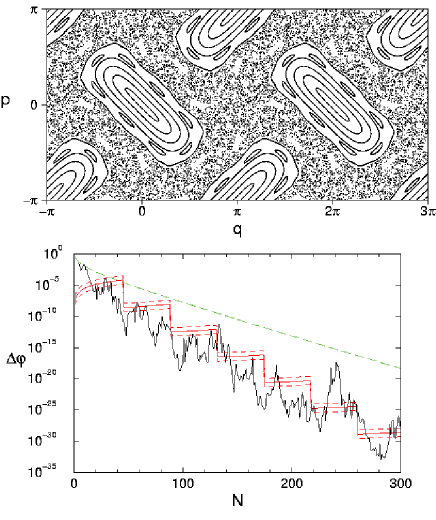
Figure 11: (Colour online) A typical mixed regular-chaotic phase space obtained for the kicked Harper map with $\tau=2$ is shown in the upper panel. A prominent $8$:$2$ nonlinear resonance is visible. The lower panel shows the quantum eigenphase splittings calculated for the ground state within the regular island as a function of $N\equiv 2\pi/\hbar$. The thick solid line (red) is the semiclassical prediction based on the $8$:$2$ resonance for the average splittings along with the logarithimic standard deviations as dashed lines (red). The long dashed curve (green) is the Podolskiy-Narimanovpn03 prediction for the same system. Figure courtesy of P. Schlagheck.

The mechanism for CAT just outlined has been confirmed for a variety of systems. Eltschka and Schlagheck confirmed that the plateau structures appear for the kicked rotor case as well. Wimberger et al. very recently showedwseb06 that the decay of the nondispersive electronic wavepackets in driven ionizing Rydberg systems is also controlled by the RAT mechanism. Mouchet et al. performed a fairly detailed analysis of an effective Hamiltonian that can be realized in experiments on cold atoms and provide clear evidence for the important role played by the various nonlinear resonancesmes06 . A extensive studysfgr06 , by Sheinman et al., of the lifetimes associated with the decay of the quantum accelerator modes revealed regimes wherein the RAT mechanism is crucial. In this context it is interesting to ask wether the mechanism would also explain the CAT process in the Bohigas-Tomsovic-Ullmo system described by the Hamiltonian in Eq. (28). It is evident from the inset in Fig. 8b that nonlinear resonances do show up around the chaos-regular border but a systematic study of the original system from the recent viewpoints is yet to be done. Similar questions are being addressedss07 in the Lin-Ballentine system (cf. Eq. (27)) i.e., to what extent is the decay of a coherent state localized in the center of the regular island controlled by the RAT mechanism. Naturally, in cases wherein the regular islands are “resonance-free” the RAT mechanism is absent. A recent example comes from the work of Feist et al. on their studiesfbkrhb06 on the conductance through nanowires with surface disorder which is controlled by dynamical tunneling in a mixed phase space.

Thus based on the numerous systems studied there are clear indications that the nonlinear resonances are indeed important to understand the CAT mechanism. Nevertheless certain observations reveal that one does not have a full understanding as of yet. For instance it is clear from Fig. 11 that the semiclassical theory underestimates the exact quantum splittings in the regimes of large $\hbar$. This could be due to the fact that the key nonlinear resonance, on which the estimate is based, is not clearly resolved. It could also be due to the fact that within the pendulum approximation the action dependence of the Fourier coefficients are neglected. Alternatively it is possible that a different mechanism is operative at large $\hbar$ and in particular the Podolskiy-Narimanov theory might be relevant in this context. However, as evident from the results reported in the recent workmes06 by Mouchet et al., the Podolskiy-Narimanov estimate tends to overestimate in certain systems. In this context note that Sheinman has recently derivedsheinthesis , using assumptions identical to those of Podolskiy and Narimanov, an expression for $\Delta E$ which differs from the result in Eq. (32). Moreover the assumption of neglecting the action dependencies of the Fourier coefficients in Eq. (35) needs to be carefully studied especially in cases wherein the nonlinear resonances are rather large.

A more crucial issue pertains to the role played by the partial barriers like cantori at the regular-chaotic border. At present the RAT based mechanism still assumes the border to be devoid of such partial barriers and thus models the chaotic part by a random hermitian matrix. As briefly mentioned in the introduction the partial barriers do play an important role in the molecular systems as well. In this context the studiesbw861 ; bw862 by Brown and Wyatt on the driven Morse oscillator are highly relevant. The driven Morse system, a model for the dissociation dynamics of a diatomic molecule, clearly points to the crucial role of the cantori in the quantum dynamicsbw861 ; bw862 . Interestingly the dissociation dynamics of the driven Morse system can be analysed from a dynamical tunneling perspective to understand the interplay of nonlinear resonances, chaos, and cantori in the underlying phase space. Investigations along these lines are in progress. Currently there is no theory which combines the RAT viewpoint with the effect of the hierarchical structures located in the border regions of the phase spacepsprivate .

V Consequences for IVR

Notwithstanding the issues raised in the previous sections, the key point in the context of this review has to do with the relevance of the RAT and CAT phenomena to IVR. Heller in his stimulating reviewHel95 raised several questions regarding the manifestation of dynamical tunneling in molecular spectra. It is thus interesting to ask as to what extent has the recent progress contributed towards our understanding of quantum mechanisms for IVR. This section therefore summarizes the recent progress from the molecular standpoint.

The Hamiltonians used in this section are effective spectroscopic Hamiltonians of the form given in Eq. (3). The origin and utility of the effective Hamiltonians have already been discussed in the introduction. Three reasons are worth stating at this juncture. Firstly, the classical limit of the spectroscopic Hamiltonians are very easily constructed. Secondly, the various nonlinear resonances are specified and hence it is possible to perform a careful analysis of the role of the resonances and chaos in dynamical tunneling. A third reason has to with the fact that effective Hamiltonians of similar form arise in different contexts like electron transfer through molecular bridgesNitz01 , coupled Bose-Einstein condensates, and discrete quantum breathersffo01 ; df02 ; pf06 . Interestingly the notion of local modes has close connections with the existence of discrete breathers or intrinsic localized modes which have been, and continue to be, studied by a number of researchersFle03 ; cfk04 . Wether the intrinsic localized modes can exist quantum mechanically is nothing but the issue of dynamical tunneling in such discrete systems. Therefore one anticipates that techniques of the previous sections should be useful in studying the breather-breather interactions as well. Indeed a recent work by Dorignac et al. invokesdess04 the appropriate off-resonant states to couple the degenerate states.

V.1 Local mode doublets

To illustrate the RAT and CAT phenomena recent studies focus on the effective local mode HamiltonianBag88

$$H=H_{0}+g^{\prime}V_{1:1}^{(12)}+\gamma V_{2:2}^{(12)}+\frac{\beta}{2\sqrt{2}}(V_{2:1}^{(1b)}+V_{2:1}^{(2b)})$$ (49)

with $g^{\prime}=g+\lambda^{\prime}(n_{1}+n_{2}+1)+\lambda^{\prime\prime}n_{b}$, describing the highly excited vibrational states of a ABA triatomic. In the above the local mode stretches are denoted by $(1,2)$ and the bending mode is denoted by $b$. As stated previously such systems were one of the first ones to highlight the manifestation of dynamical tunneling in molecular spectra. Here, however, the bending mode is included and thus allows for several anharmonic resonances and a mixed phase space. The zeroth-order anharmonic Hamiltonian is

$$H_{0} = \omega_{s}(n_{1}+n_{2})+\omega_{b}n_{b}+x_{s}(n_{1}^{2}+n_{2}^{2})+x_{b}n_{b}^{2}$$ (50)

$$+ x_{sb}n_{b}(n_{1}+n_{2})+x_{ss}n_{1}n_{2}$$

with $n_{j}=a_{j}^{\dagger}a_{j}$ being the occupation number of the $j$-th mode written in terms of the harmonic creation $(a_{j}^{\dagger})$ and the destruction $(a_{j})$ operators. The zeroth-order states $|n_{1},n_{2},n_{b}\rangle$ are coupled by the anharmonic resonances of the form

$$V_{p:q}^{(ij)}=(a_{i}^{\dagger})^{q}(a_{j})^{p}+(a_{j}^{\dagger})^{p}(a_{i})^{q}$$ (51)

Thus $V_{p:q}^{(ij)}$ couples states $|{\bf n}\rangle$ and $|{\bf n}^{\prime}\rangle$ with $|n_{i}^{\prime}-n_{i}|=q$ and $|n_{j}^{\prime}-n_{j}|=p$. Due to the structure of the Hamiltonian the polyad number $P=(n_{1}+n_{2})+n_{b}/2$ is exactly conserved and thus the system has effectively two degrees of freedom.

Table 1: Local mode splittings in cm^-1 for H₂O

State	$\Delta E_{expt}$	$\Delta E_{b}$
$(10^{\pm})0$	98.876	100.26
$(20^{\pm})0$	48.278	48.407
$(30^{\pm})0$	13.669	12.919
$(40^{\pm})0$	2.661	2.334
$(50^{\pm})0$	0.442	0.514
$(60^{\pm})0$	0.105	0.134
$(70^{\pm})0$	0.145	0.013

The Hamiltonian has been proposed by BaggottBag88 to fit the vibrational states of H₂O and D₂O for specific choice of the parameters of $H$. A comparison of the local mode splittings predicted using the Baggott Hamiltonian and the recent experimental datatenny of Tennyson et al. is shown in the table  1. The agreement is quite good considering the fact that the polyad $P$ perhaps breaks down at higher levels of excitations. Another reason for the choice of the system had to do with the fact that the classical-quantum correspondence for the Hamiltonian in Eq. (49) was already well established from several earlier workske95 ; ke97 ; lk97 . Additional motivation has to do with the possibility of studying the RAT and the CAT mechanisms in a controlled fashion by analysing the following sub-HamiltoniansKes05 :

$$H_{A} = H_{0}+\frac{\beta}{2\sqrt{2}}(V_{2:1}^{(1b)}+V_{2:1}^{(2b)})$$ (52)

$$H_{B} = H_{A}+\gamma V_{2:2}^{(12)}$$ (53)

The Hamiltonian $H_{A}$ for smaller polyads exhibits near-integrable dynamics. The same is true for $H_{B}$ but with an additional weak $2$:$2$ resonance and hence it is possible to study the influence of multiple nonlinear resonances. On the other hand the full Hamiltonian $H$ has a mixed regular-chaotic phase space and thus on going from $H_{A}\rightarrow H_{B}\rightarrow H$ a systematic study of the influence of phase space structures on dynamical tunneling is possible. The classical limit can be obtained using the correspondence

$$a_{j}^{\dagger}\leftrightarrow\sqrt{I_{j}}\exp(i\theta_{j})\,\,\,\,;\,\,\,\,a_{j}\leftrightarrow\sqrt{I_{j}}\exp(-i\theta_{j})$$ (54)

and yields a nonlinear multiresonant Hamiltonian in terms of the action-angle variables of the zeroth-order $H_{0}$. For instance the resonant perturbation Eq. (51) has the classical limit

$$V_{p:q}^{(ij)}\rightarrow V_{p:q}({\bf I},{\bm{\theta}})=2(I_{i}^{q}I_{j}^{p})^{1/2}\cos(q\theta_{i}-p\theta_{j})$$ (55)

with the obvious correspondence ${\bf I}\rightarrow({\bf n}+1/2)\hbar$.

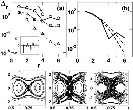
Figure 12: (a) Local mode doublet splitting $\Delta_{r}$ in cm^-1 with increasing excitation quantum $r$ for polyad $P=6$. The exact quantum (lines) are compared to the vibrational superexchange (symbols) at minimal order. Note that the agreement is excellent except for the $r=4$ case for the full Hamiltonian (solid line). Inset shows the contribution from $130$ different coupling chains towards obtaining $\Delta_{6}$ in case A. (b) $\Delta_{r}$ estimated from the $1$:$1$ nonlinear resonance alone (dashed) and the $1$:$1$+$2$:$2$ resonances (dot-dashed) compared with the full case (solid line). Note that the Hamiltonian with $1$:$1$ and $1$:$1$+$2$:$2$ are classically integrable. The three lower panels show the phase space $(K_{1}/2,\phi_{1}/4\pi)$ at increasing energies corresponding to $r=2,3$, and $4$ for Eq. (49). Significant amount of chaos and the $2$:$1$ stretch-bend nonlinear resonances set in for $r=4$.

The zeroth-order states $|n_{1}=r,n_{2}=0,n_{b}=2(P-r)\rangle\equiv|r,0\rangle$ and $|0,r\rangle$ are degenerate in the absence of the resonant couplings. However, in the presence of the couplings the degeneracy is broken resulting in the local mode doublets with a splitting $\Delta_{r}$. In other words if an initial state $|r,0\rangle$ is prepared then on a time scale of $T=2\pi/\Delta_{r}$ the population is completely trasferred to the symmetric partner state $|0,r\rangle$. This corresponds to a dynamical tunneling process since there are no energetic barriers to be blamed in this caseKes05 . Quantum mechanically for a given polyad $P$ the splittings can be obtained easily by diagonalizing a $N\times N$ matrix with $N=(P+2)(P+3)/2$. The superexchange calculation in this multiresonant case is more involved than in the single resonance case. One important consequence of the multiresonant couplings is that the number of coupling chains connecting $|r,0\rangle$ and $|0,r\rangle$ in the state space for a given $P$ is infinite. It turns outKes03 that the minimal order estimate

$$\Delta_{r}=\sum_{abc}\beta^{a}g^{\prime b}\gamma^{c}\sum_{\mu}\Delta_{r}(\Gamma_{abc}^{(\mu)})$$ (56)

provides a very good approximation to the exact quantum splittings. The index $\mu$ labels all possible coupling chains $\Gamma_{abc}$ for a specific choice of $a,b$, and $c$ satisfying the constraint $a+2b+4c=2r$. The contribution to the overall splitting from a specific coupling chain, which has the form as in Eq. (24), is denoted by $\Delta_{r}(\Gamma_{abc}^{(\mu)})$. The expression in Eq. (56) is nothing but the lowest order of perturbation that would connect the two degenerate states involving a net change $\Delta{\bf n}\equiv|{\bf n}-{\bf n}^{\prime}|=2r$. The excellent agreement between the exact quantum and the superexchange calculation for $P=6$ is shown in Fig. 12a for the actual system and the various subsystemsKes05 . Note that in case of $H_{A}$ a superexchange calculation of $\Delta_{6}$ involves twelfth-order perturbation with $130$ coupling chains of varying signs, some as large as $10^{-4}$, conspiring to yield a fairly accurate value. In Fig. 12b the splittings are calculated by retaining only the $1$:$1$ resonance or the $1$:$1$+$2$:$2$ resonances. The $\Delta_{r}$ monotonically decrease in both cases with increasing $r$ i.e., OH-stretch excitations as observed earlier. However starting with $r=4$ the integrable subsystem cannot account for the exact splittings. In particular the exact case exhibits nonmonotonic behaviour which neither the integrable limit cases nor the superexchange calculation can predictKes03 ; Kes05 . On the other hand the monotonic trend seen in Fig. 12a for the near-integrable subsystems is not true in general. For instance in an earlier workKes03 strong fluctuations were seen in the near-integrable case for $P=8$. It is well known that such fluctuations have to with the avoided crossings of the doublets with one or more states. The avoided crossings can occur in near-integrable (see Fig. 9 for example) as well as in the mixed phase space situations. The phase space for the full Baggott Hamiltonian is shown in Fig. 12 with increasing energy. The surface of sections are shown in the canonically conjugateke97 variables $(K_{1}/2,\phi_{1})\equiv((I_{1}-I_{2})/2,(\theta_{1}-\theta_{2})/2)$ at fixed sectioning angle $\phi=\theta_{1}+\theta_{2}-4\theta_{b}$ with $\dot{\phi}>0$. The normal mode regions appear around $I_{1}\sim I_{2}$. The appearance of significant amount of chaos and the $2$:$1$ stretch-bend resonances in the phase space at higher energies suggests that the RAT and, to some extent CAT, mechanisms could explain the various results.

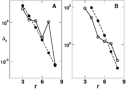
Figure 13: Local mode splittings in cm^-1 for the polyad $P=8$ for (A) H₂O and (B) D₂O using the appropriate parameters in the full Hamiltonian of Eq. (49). The open circles denote the exact quantum values whereas the filled circles represent a semiclassical calculation using an integrable approximation. Note that the integrable approximation decays monotonically in both cases and fails to account for the fluctuations. The phase space is mixed regular-chaotic for both the molecules but the fluctutations in $\Delta_{r}$ are muted in D₂O.

As another example, in Fig. 13 the local mode splittings computed using Eq. (49) for parameters appropriate to H₂O and D₂O and a higher polyad $P=8$ are shown. It is clear that the splittings for a given local mode state are typically larger for D₂O as compared to H₂O. Note that this immediately establishes the dynamical nature of the tunneling since usual arguments of isotopic substitution invoked for the potential barrier tunneling cases would predict the opposite. This, of course, is not surprising since the dynamical tunneling involves transfer of vibrational quanta as opposed to the transfer of atoms. In addition the enhanced splittings for D₂O is consistent with the fact that H₂O is a better local mode system than D₂O. The phase space for both systems are mixed regular-chaotic and similar to that shown in Fig. 12. Does the nonintegrability of the system dynamics, and hence the chaos, have any impact on the local mode splittings? In order to address the question the splittings are computed for an integrable approximation to the Baggott Hamiltonian. The splittings computed using the integrable approximation are compared to the exact splittings in Fig. 13 for both the molecules. The integrable limit splittings, as expected, decay monotonically with increasing excitation. Although the comparison looks favorable, except for the nonmonotonicity, for H₂O it is clear from Fig. 13 that similar levels of agreement are not seen for D₂O. More importantly, the fluctuations in $\Delta_{r}$ are completely missed and thus suggest that the exact splittings are determined by a subtle interplay of the nonlinear resonances and chaos.

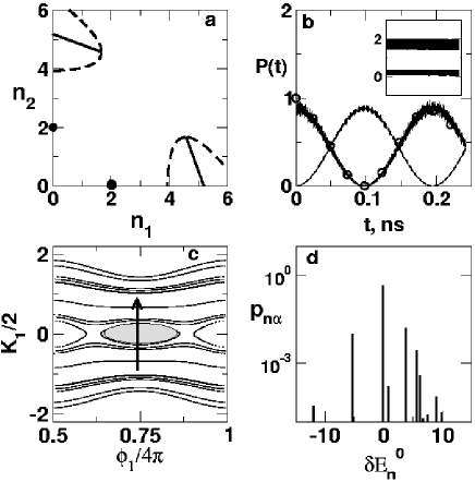
Figure 14: (a) State space $(n_{1},n_{2})$ for $P=6$ with the location of the $2$:$1$ stretch-bend nonlinear resonance zones (dashed regions) shown for reference. (b) Quantum survival probability for the state $|2,0\rangle$ (circles) computed using $H_{A}$ shows two-level like mixing with the symmetric partner $|0,2\rangle$ despite trapping of classical trajectory on the same timescale (inset). Thus the quantum energy transfer is due to dynamical tunneling. (c) RAT mechanism due to the $1$:$1$ nonlinear resonance (shaded) in the phase space induced by the remote $2$:$1$s explains the energy flow. (d) Overlap intensities versus $\delta E_{\bf n}^{0}\equiv(E_{\alpha}-E_{\bf n}^{0})$ (in units of mean level spacing) shows involvement of off-resonant states.

To illustrate RAT consider the mixing between the zeroth-order states $|2,0\rangle$ and $|0,2\rangle$ due to the stretch-bend resonance in $H_{A}$. The states are not coupled directly by the resonances as can be inferred by the state space shown in Fig. 14a. The resonance zones, computed using the Chirikov approximationChi79 , are quite far from the states. Indeed Fig. 14b shows that the classical dynamics exhibits trapping, however the quantum survival probability of $|2,0\rangle$ shows complete mixing with $|0,2\rangle$ on a time scale of about $0.1$ nanoseconds. As before off-resonant states participate in vibrational superexchange, clear from Fig. 14d, resulting in the observed mixing. There are now several coupling chains at minimal order and the perturbative calculation yields $\Delta_{2}\approx 0.18$ cm^-1 in excellent agreement with the exact value (cf. Fig. 12). What is the role of the stretch-bend resonances? This becomes clear on looking at the phase space for $H_{A}$ at $E=E_{2,0,8}^{0}$ shown in Fig. 14c. One immediately notices a nonlinear resonance located between the phase space regions corresponding to the two states. The resonance however is not the $2$:$1$ stretch-bend resonance but a weak $1$:$1$ resonance between the local stretches induced by the stretch-bend couplings. It can be shownKes05 using classical perturbation theoryllbook that the induced $1$:$1$ is governed by a pendulum Hamiltonian of the form

$$H(K_{1},\phi_{1};K_{2},N)=\frac{K_{1}^{2}}{2M_{11}}+2g_{\rm ind}(K_{2},N)\cos(2\phi_{1})$$ (57)

with $K_{2}\equiv I_{1}+I_{2}$ ($1$:$1$ subpolyad) and $N\equiv(I_{1}+I_{2})+I_{b}/2$ (classical analog of the polyad $P$) being the approximately and exactly conserved quantities. The parameters appearing in the pendulum Hamiltonian can be expressed in terms of the parameters of the original Hamiltonian asKes05

$$M_{11} = 2(\alpha_{12}-2\alpha_{ss})^{-1}$$ (58a)

$$g_{\rm ind} = \frac{\beta^{2}}{4}K_{2}(N-2K_{2})f(K_{2},N)$$ (58b)

$$f(K_{2},N) = \left\{\frac{4(\Omega_{s}+\alpha_{ss}K_{2})+\alpha_{12}N}{[2(\Omega_{s}+\alpha_{ss}K_{2})+\alpha_{12}K_{2}]^{2}}\right\}$$ (58c)

where the parameters $\Omega_{s},\alpha_{ss}$, and $\alpha_{12}$ are related to the original parameters of Eq. (49). The induced coupling strengthtypojcp05 is related to the width of the resonance island seen in Fig. 14c. Thus having idenitified the key resonance the splitting between a general local mode pair can be estimated as

$$\frac{\Delta_{r}^{\rm sc}}{2}=g_{\rm ind}\prod_{k=-(r-2)}^{(r-2)}\frac{g_{\rm ind}}{E_{r}^{0}-E_{k}^{0}}=\frac{g_{\rm ind}}{[(r-1)!]^{2}}\left(\frac{M_{11}g_{\rm ind}}{2}\right)^{r-1}$$ (59)

with $E_{j}^{0}=j^{2}/2M_{11}$ being the unperturbed energy from Eq. (57). Using parameters appropriate for H₂O in Eq. (49) and the expressions in Eq. (58c) one obtains $M_{11}\approx 1.32\times 10^{-2}$ and $g_{ind}\approx 3.93$ cm^-1. Thus $\Delta_{2}^{sc}\approx 0.20$ cm^-1 which is in agreement with the exact and superexchange values. This clearly supports the RAT mechanism for the quantum mixing seen in Fig. 14b.

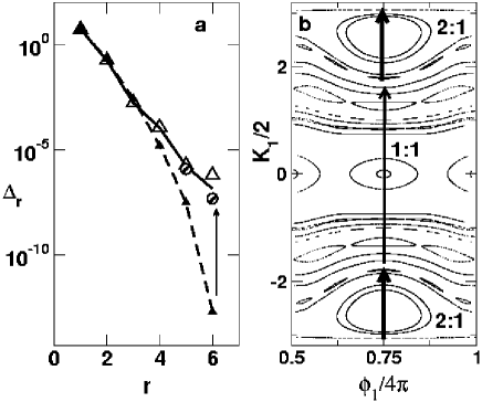
Figure 15: (a) Splittings in cm^-1 for $P=6$ overtone states for $H_{A}$. The exact result (solid line), superexchange calculation (open triangles), and predictions based on the induced $1$:$1$ stretch-stretch resonance alone (filed triangles, dashed line) are compared. (b) Phase space for $H_{A}\approx E_{6,0,0}^{0}$ emphasizes the need for invoking multiple resonances (arrows). RAT mechanism using the multiple resonances leads to very good agreement shown in (a) as shaded cricles.

Although the classical dynamics of $H_{A}$ is near-integrable the phase space can be very rich in terms of several resonances. The RAT mechanism depends on identifying the crucial resonances. In Fig. 12 the monotonic decrease of $\Delta_{r}$ with $r$ for the system described by $H_{A}$ and $H_{B}$ might suggest that the induced resonance alone controls the splittings. However Fig. 15a shows that calculating the splittings using Eq. (57) yields very poor results for $r=5,6$. The reason becomes clear on inspecting the phase space and Fig. 15b shows the case of $r=6$ as an example. The Husimi distribution of the state $|6,0,0\rangle$ would be localized about $K_{1}\approx 6$ and thus the $2$:$1$ stretch-bend and the $1$:$1$ induced resonance islands seperate the state from its symmetric partner $|0,6,0\rangle$ localized around $K_{1}\approx-6$. Several other resonances are also visible at this energy in Fig. 15b but they are of higher order and perhaps not relevant for large $\hbar$ values. Moreover the Husimi representations indicateKes05 that the state $|5,0,2\rangle$ is localized inside the $2$:$1$ island (ground state) and the state $|4,0,4\rangle$ corresponds to the separatrix state. Thus the $2$:$1$ resonance must be coupling the $|6,0,0\rangle$ and $|4,0,4\rangle$ states. As a consequence the RAT mechanism can be schematically written as

$$|6,0\rangle\stackrel{{\scriptstyle\beta_{\rm eff}}}{{\longrightarrow}}|4,0\rangle\stackrel{{\scriptstyle g_{\rm ind}}}{{\longrightarrow}}|0,4\rangle\stackrel{{\scriptstyle\beta_{\rm eff}}}{{\longrightarrow}}|0,6\rangle$$ (60)

with $\beta_{\rm eff}$ being the effective coupling across the $2$:$1$ islands and $g_{\rm ind}$ being the effective $1$:$1$ coupling in Eq. (58c) for $r=6$. This is illustrated in Fig. 15b on the phase space as well. Again approximating the $2$:$1$ islands by pendula it is possibleKes05 to determine the $\beta_{\rm eff}$ and the computed splittings agree rather well with the exact results as shown in Fig. 15a. Thus Fig. 15 demonstrates the RAT mechanism in that the mixing between two remote (both in state space and the phase space) states $|6,0,0\rangle$ and $|0,6,0\rangle$ is characterized by the nonlinear resonances. Further confirmation of the multiresonant mechanism comes from the fact that values of $\Delta_{6}$ for $H_{B}$ and the full Hamiltonian also compare well with the exact results. The subtelty of the mechanism lies in the fact that all the nonilinear resonances in Fig. 15b arise from the two $2$:$1$ resonances and at smaller values of $\hbar$ one expects the higher order resonances to come into play.

Figure 16: Variations in the splittings for the ground state of the $2$:$1$ island with coupling strength $\beta$. (a) Effect of breaking the polyad by adding weak $3$:$1$ resonance to $H$ with strength $\delta=0.1$ cm^-1 (circles) contrasted with the polyad conserved ($P=16$) case (thick line). The phase space (with axes as in Fig. 12) is shown in the latter case for select values of $\beta$. (Inset) Fluctuations in the splitting for $P=8$ case (thick line) compared to that with $\hbar$ reduced by half (circles). All quantities are in units of cm^-1.

The role of RAT in explaining the local mode doublet splittings is obvious from the preceeding discussion and examples. Model studies reveal that even very small, on the scale of $\hbar$, nonlinear resonances mediate dynamical tunneling in molecular systemsKes05 . However the role of CAT is far from being established and some of the issues involved were highlighted before in this review. In essence, to implicate CAT atleast a third chaotic state has to be identifiedbtu93 ; tu94 . Moreover the system should be in the deep semiclassical limit i.e., small enough $\hbar$ so that the quantum dynamics can sense the presence of chaos in phase space. These are fairly severe constraints and experimentally there are not many systems which respect the constraints. Intutively speaking, highly excited energy regions of moderate sized molecules might be ideal systems. One possibility is that the signatures of CAT could be present in the eigenstates of highly excited molecules and could potentially complicate the state assignments. One such example can be found in the workke95 by Keshavamurthy and Ezra on the dynamical assignments of the highly excited states of H₂O for $P=8$. Another example, perhaps, can be found in the workjjtw99 by Jacobson et al. wherein the highly excited ($\sim$ 15000 cm^-1 above the ground state) vibrational states of acetylene are dynamically assigned. In their study Jacobson et al. found that approximate assignments could be done in an energy range which had highly chaotic phase space whereas many of the eigenstates could not be assigned in another energy range despite the existence of large regular regions in the phase space. To some extent an indirect role of CAT is evident from Fig. 12b wherein the dominant integrable resonances cannot account for the exact splittings. Some more hints originate from Fig. 16 where the fluctuations in the splittings associated with the ground state of the $2$:$1$ island are shown in two different situations. The first of these investigates the effect of breaking the polyad constant $P$ by adding weak $3$:$1$ stretch-bend resonances to the Hamiltonian in Eq. (49). Thus the three degrees of freedom Hamiltonian is

$$H_{3d}=H+\delta(V_{3:1}^{(1b)}+V_{3:1}^{(2b)})$$ (61)

with $\delta=0.1$ cm^-1 which is three orders of magnitude smaller than the mean level spacing of $H$. A consequence of $\delta\neq 0$ is that the effective density of states is increased providing many more states with different $P$ to interact with the state of interest. In Fig. 16 the effect of such a small perturbation is shown for $P=16$ and clearly there are far more fluctuations in the mixed regime. However away from the fluctuations the inverse participation ratio of the state is nearly one in the basis of the two degrees of freedom Hamiltonian $H$ which suggests minor influence of states with $P\neq 16$. Despite this and the weak coupling strength $\delta$ there are significant differences between the computed splittings for $H_{3d}$ and $H$. Presumably this has to do with the subtle changes in the nature of the chaotic states upon adding the $3$:$1$ resonances but further studies are required in order to gain a better understanding. The results of a second system shown in the inset to Fig. 16 reveal the increased flutuations in the splittings for the state with $P=8$ on decreasing the value of $\hbar$ by half. Interestingly in this case the average splitting seems to decrease with increasing $\beta$ and thus increasing stochasticity in the phase space.

Most of the detailed phase space studies have focused on the role played by classical phase space structures for vibrational modes alone. The involvement of rotations, torsions, and other large amplitude modes in molecular systems and their implications for IVRkmp00 and dynamical tunneling have received relatively less attention. Early pioneering studieshp84 by Harter and Patterson showed that the splitting of the doubly degenerate $K$-levels of a symmetric top on the introduction of asymmetry could be associated with tunneling across a separatrix on the so called rotational energy surface. Would the coupling of vibrations to these other modes enhance or suppress the splittings? Harter has extended the rotational energy surfaces idea to describe and interpret the dynamics and spectra for a class of anharmonic coriolis coupled vibrational modesHar86 . Lehmann studiedLeh91 ; Leh92 the coupling of rotations to the local mode vibrations in XH_n systems. In particular Lehmann, and independently Child and Zhucz91 , considered the modification of the local mode dynamical tunneling due to the interactions with rotations. Depending on the local mode tunneling time the rotation motion would reflect the extent of dynamical symmetry of the local mode state. Interestingly Lehmann’s analysis reveals that it is possible for the rotation of a molecule to significantly reduce the tunneling rate i.e., decrease the doublet splittingLeh91 . Such rotational quenching of the local mode tunneling is due to the fact that in addition to the transfer of vibrational quanta it is also necessary to reorient the angular momentum in the body fixed frame. Semiclassical insights arise by looking at the motion on the rotational energy surfaces. It is not clear as to how much of a role does the classical chaos plays in the studies of Harter and Lehmann. However, the local mode splitting is determined by RAT and CAT mechanisms and hence they also determine the timescales relative to rotations. It remains to be seen if the different mechanisms are reflected in the nature of the rovibrational eigenstates. A possible signature of CAT was suggestedOrt96 by Ortigoso nearly a decade ago. Ortigoso found anomalously large $K$-splittings for some of the asymmetry doublets occuring in the rotation-torsion energy levels of acetaldehyde. Further studies involving coupling with vibrations have not been undertaken although, based on time scale separations one can argue that the observed enhancements might lead to increased vibration-rotation couplings with important consequences for IVR.

V.2 State mixing in multidimensions

Every single example in this section up until now has involved systems with discrete symmetry and two degrees of freedom. The requirement of discrete symmetries for dynamical tunneling is not very restrictive. As discussed before in this review this aspect has been emphasized in the early work as well. TomsovicTom98 has also discussed the possibility of observing CAT in the absence of reflection symmetries. On the other hand studies on dynamical tunneling in systems with large degrees of freedom are crucial. Given that there are important differencesllbook , briefly mentioned in the introduction, between the classical dynamics in two and more than two degrees of freedom it is natural to ask if the RAT and CAT mechanisms hold in general. Especially from the IVR perspective the crucial question is wether dynamical tunneling can provide a route for mixing between near-degenerate states and hence energy flow between phase space regions supporting qualitatively different types of motion. Thus is it possible that an excited CH-stretch can, over long times, evolve into a CC-stretch despite the lack of any obvious coupling? Heller and Davis conjectureddh812 that it should be possible and the agent would be dynamical tunneling. However support for the conjecture from a phase space viewpoint have not been forthcoming.

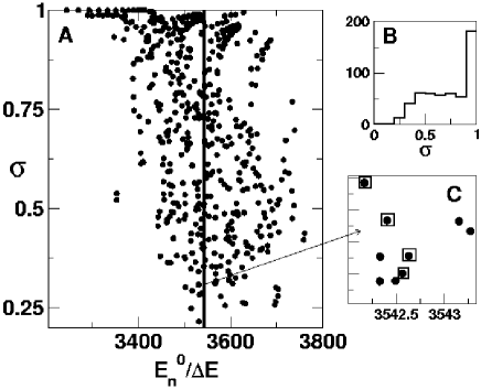
Figure 17: (A) Dilution factors $\sigma$ of the zeroth-order states $|{\bf n}\rangle$ with $H_{0}|{\bf n}\rangle=E_{\bf n}^{0}|{\bf n}\rangle$ versus energy for the Hamiltonian in Eq. (62). The polyad value is $P=8$ and couplings $0.5K_{{\bf m}_{1}}=K_{{\bf m}_{2}}=K_{{\bf m}_{3}}\approx 0.2\Delta E$ with mean level spacing $\Delta E\approx 4.4$ cm^-1. (B) Histogram showing the distribution of $\sigma$ in (A). Note that a large number of states have unit dilutions but there are also a number of states with $\sigma<1$ indicating mixing of the zeroth-order states. Is the mixing due to dynamical tunneling? In (C) an expanded view of the states around $\bar{E}\approx 3542.5\Delta E$ in (A) is shown. Four states of interest are highlighted by squares.

A first step towards such goals was recently takenKes051 by studying the model Hamiltonian

$$H=H_{0}+\sum_{r}K_{{\bf m}_{r}}\left[(a_{1}^{\dagger})^{\alpha_{r}}(a_{2})^{\beta_{r}}(a_{3})^{\gamma_{r}}(a_{4})^{\delta_{r}}+h.c.\right]$$ (62)

describing four coupled modes $j=1,2,3,4$ with the zeroth-order part

$$H_{0}=\sum_{j}(\omega_{j}n_{j}+x_{jj}n_{j}^{2})+\sum_{j<k}x_{jk}n_{j}n_{k}$$ (63)

The zeroth-order states $|{\bf n}\rangle$, eigenstates of $H_{0}$ with eigenvalues $E_{\bf n}^{0}$, get coupled and hence mixed due to the anharmonic resonances chracterized by ${\bf m}_{r}=(\alpha_{r},-\beta_{r},-\gamma_{r},-\delta_{r})$ with strengths $K_{{\bf m}_{r}}$. In order to model a system without any symmetries the parameters of $H_{0}$ were taken from the workbhmqs00 of Beil et al. corresponding to the four high frequency modes of the molecule CDBrClF. Three perturbations ${\bf m}_{1}=(1,-2,0,0),{\bf m}_{2}=(1,-1,-1,0)$, and ${\bf m}_{3}=(1,-1,0,-1)$ with very weak strengths $K_{{\bf m}_{r}}/\Delta E\equiv k_{{\bf m}_{r}}<1$, relative to the mean level spacing $\Delta E$, are selected. Note that the coupling structure of the Hamiltonian implies the existence of a good polyad quantum number $P=n_{1}+(n_{2}+n_{3}+n_{4})/2$. Thus the model Hamiltonian has effectively three degrees of freedom.

A few words about the choice of the Hamiltonian is perhaps appropriate at this stage. Firstly, the form of $H_{0}$ is quite generic and the parameters were chosen from an experimental fitbhmqs00 in order to test the ideas on a real molecular system. Secondly the Hamiltonian in Eq. (62) can be considered to be in the intrinsic resonance representationchm97 . In other words the Hamiltonian models the weak residual couplings between the KAM tori corresponding to $H_{0}$. Finally the choice of the resonant couplings is also arbitrary; a different set of couplings would generate mixings among different zeroth-order states.

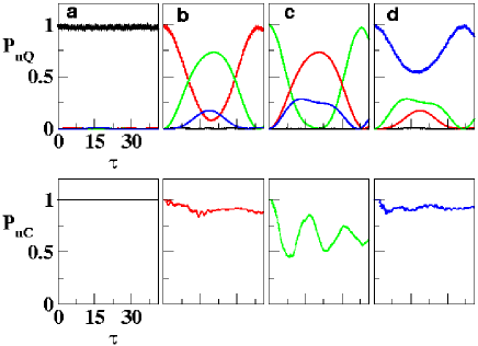
Figure 18: (Colour online) Quantum (top panel) and classical (bottom panel) survival probabilities of the four zeroth-order states shown in Fig. 11C. Parameters chosen are as in Fig. 11. Time $\tau$ is measured in units of the Heisenberg time $\tau_{H}=(2\pi c\Delta E)^{-1}$. State $|a\rangle$ (black) shows long time trapping in both cases. States $|b\rangle$ (red), $|c\rangle$ (green), and $|d\rangle$ (blue) mix amongst each other quantum meachanically in contrast to their classical behaviour. The quantum cross probabilities $|\langle{\bf n}^{\prime}|{\bf n}(t)\rangle|^{2}$ are also shown with consistent color coding. Adapted from ref. Kes051, .

The relevant issue here has to do with the fate of zeroth-order states $|{\bf n}\rangle,|{\bf n}^{\prime}\rangle,\ldots,$ which are near-degenerate $E_{\bf n}^{0}\approx E_{{\bf n}^{\prime}}^{0}\approx,\ldots,$ in the presence of such weak perturbations. In Fig. 17A the dilution factors for the various zeroth-order states are shown and it is clear that many zeroth-order states are mixed. In particular within one mean level spacing several states have varying levels of mixing and a typical example is shown in Fig. 17C. Is the mixing observed in Fig. 17C due to dynamical tunneling? In order to check four states are picked and correspond to $|a\rangle=|0,11,1,4\rangle,|b\rangle=|0,11,2,3\rangle,|c\rangle=|0,12,2,2\rangle$, and $|d\rangle=|0,13,1,2\rangle$. The choice of the energy range and the states is fairly arbitrary as evident from Fig. 17. First it can be confirmed by evaluating the quantum survival probability $P_{{\bf n}Q}$ and its classical analog $P_{{{\bf n}C}}$, shown in Fig. 18, that the mixing of the states of interest is indeed a quantum process i.e., classically forbidden. It is also apparent from Fig. 18 that states $|b\rangle,|c\rangle$, and $|d\rangle$ mix amongst each other over long time scales. State $|a\rangle$ on the other hand shows trapping both classically and quantum mechanically. Explanation for the observed mixings in Fig. 17 can be given in terms of the vibrational superexchange mechanism. Indeed the IVR ‘fractionation’ pattern, shown in Fig. 19, indicates a a clump of virtual or off-resonant states about $60\Delta E$ away from the corresponding ‘bright’ states. Such fractionation patterns are similar to those observed in the experimentscpcesgls03 of Callegari et al. for example. The off-resonant states have $\sigma\approx 1$ and hence do not mix significantly. However it is important to note that the fractionation pattern looks the same in case of every state and hence there must be subtle phase cancellation effect to explain the trapping exhibited by $|a\rangle$. At the same time Fig. 19 also shows that the vastly different IVR from the four states cannot be obviously related to any avoided crossing or multistate interactions.

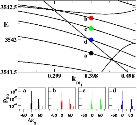
Figure 19: (Colour online) The top panel shows variation of the eigenvalues $E\equiv E_{\alpha}/\Delta E$ with the coupling parameter $k_{{\bf m}_{1}}$ with the other couplings fixed as in Fig. 11. Eigenstates having the largest contribution from the specific zeroth-order states are indicated. Bottom panel shows the ‘fractionation’ pattern i.e., overlap intensities $p_{{\bf n}\alpha}$ versus $\Delta\epsilon_{\bf n}\equiv(E_{\bf n}^{0}-E_{\alpha})/\Delta E$ on log scale. The cluster of states around $\Delta\epsilon_{\bf n}\approx 60$ are the off-resonant states that mediate the mixings seen in Fig. 17 and Fig. 18 via a vibrational superexchange mechanism. Adapted from ref. Kes051, .

In light of the conjecture of Davis and Hellerdh812 and the recent progress in our understanding of the mechanistic aspects of dynamical tunneling it is but natural to associate the near-degenerate state mixings with RAT. However how does one identify the specific resonances at work in this case? Given that the system has three degrees of freedom it is not possible to visualize the Poincaré surface of section at $H\approx\bar{E}$. In the present case the cruicial object to analyse is the Arnol’d webllbook i.e., the network of nonlinear resonances and the location of the zeroth-order states therein. Fortunately the classical limit Hamiltonian

$${\cal H}({\bf I},{\bm{\theta}}) = {\cal H}_{0}({\bf I})+2\epsilon\sum_{r}K_{{\bf m}_{r}}\sqrt{I_{1}^{\alpha_{r}}I_{2}^{\beta_{r}}I_{3}^{\gamma_{r}}I_{4}^{\delta_{r}}}\cos({\bf m}_{r}\cdot{\bm{\theta}})$$ (64)

$$\equiv H_{0}({\bf I})+\epsilon\sum_{r}K_{{\bf m}_{r}}f_{r}({\bf I})\cos({\bf m}_{r}\cdot{\bm{\theta}})$$

from Eq. (62) is easily obtained, as explained earlier, in terms of the action-angle variables $({\bf I},{\bm{\theta}})$ of $H_{0}$. In the above equation the variable $\epsilon$ is introduced for convenience during a perturbation analysis of the Hamiltonian. The ‘static’ Arnol’d web at $E\approx\bar{E}$ and fixed polyad $P_{c}\equiv I_{1}+(I_{2}+I_{3}+I_{4})/2$, classical analog of the quantum $P$, can then be constructed via the intersection of the various resonance planes ${\bf m}_{r}\cdot\partial{\cal H}_{0}({\bf I})/\partial{\bf I}=0$ with the energy shell ${\cal H}_{0}({\bf I})\approx\bar{E}$. The static web involves all the nonlinear resonances restricted to, say, some maximum order $|\alpha_{r}|+|\beta_{r}|+|\gamma_{r}|+|\delta_{r}|\leq M$. The reason for calling such a construction as static has to do with the fact that being based on ${\cal H}_{0}$ it is possible that many of the resonances do not have any dynamical consequence. Thus, although the static web provides useful information on the location of the various nonlinear resonances on the energy shell it is nevertheless critical to determine the ‘dynamical’ Arnol’d web since one needs to know as to what part of the static web is actually relevant to the dynamics. Further discussions on this point can be found in the paper by LaskarLas93 wherein time-frequency analysis is used to study transport in the four dimensional standard map. In order to construct the dynamical Arnol’d web it is necessary to be able to determine the system frequencies as a function of time. Several techniquesmde87 ; Las93 have been suggested in the literature for performing time-frequency analysis of dynamical systems. An early example comes from the workmdu96 of Milczewski, Diercksen, and Uzer wherein the Arnol’d web for the Hydrogen atom in crossed electric and magnetic fields has been computed. A critical review of the various techniques is clearly outside the scope of this work and hence, without going into detailed discussion of the advantages and disadvantages, the wavelet based approachaw01 ; cwu03 developed by Wiggins and coworkers is utilized for constructing the web. There is, however, ample evidence that the wavelet based local frequency analysis is ideally suited for this purpose and therefore a brief description of the method follows. Classical trajectories with initial conditions satisfying ${\cal H}({\bf I},{\bm{\theta}})\approx\bar{E}$ are generated and the nonlinear frequencies $\Omega_{k}(t)$ are computed by performing the continuous wavelet transform of the time series $z_{k}(t)=\sqrt{2I_{k}(t)}\exp(i\theta_{k}(t))$:

$$L_{g}z_{k}(a,b)=a^{-1/2}\int_{-\infty}^{\infty}z_{k}(t)g^{*}\left(\frac{t-b}{a}\right)dt$$ (65)

with $a>0$ and real $b$. Various choices can be made for the mother wavelet $g(t)$ and in this work it is chosen to be the Morlet-Grossman function

$$g(t)=\frac{1}{\sqrt{2\pi\sigma^{2}}}\exp\left(2\pi i\lambda t-\frac{t^{2}}{2\sigma^{2}}\right)$$ (66)

and the parameter values $\lambda=1$, $\sigma=2$. Note that Eq. (65) yields the frequency content of $z_{k}$ within a time window around $t=b$. In many instances one is interested in the dominant frequency and hence the required local frequency is extracted by determining the scale ($a$, inversely proportional to frequency) which maximizes the modulus of the wavelet transformaw01 i.e., $\Omega_{k}(t=b)={\rm max}_{a}|L_{g}z_{k}(a,b)|$. The trajectories are followed in the frequency ratio space $(\Omega_{1}/\Omega_{3},\Omega_{1}/\Omega_{4})$ since the energy shell, resonance zones, and the location of the zeroth-order states can be projected onto the space of two independent frequency ratios. Such ‘tune’ spaces have been constructed and analysed before, for instance, by Martens, Davis, and Ezra in their seminal workmde87 on IVR in the OCS molecule. A density plot is then created by recording the total number of visits by the trajectories to a given region of the ratio space. Quite naturally the density plot highlights the dynamically significant portions of the Arnol’d web at a given energy and polyad. The computation of such a dynamical web is shown in Fig. 20 at an energy $\bar{E}$ corresponding to the zeroth-order states of interest. One immediately observes that apart from highlighting the primary resonances Fig. 20 shows the existence of higher order induced resonances. More importantly the zeroth-order states are located far away from the primary resonances and thus the state mixings cannot be ascribed to the direct couplings in the Hamiltonian. However, the states are located in proximity to the junction formed by the weak induced resonances denoted as ${\bf m}_{i1},{\bf m}_{i2}$, and ${\bf m}_{i3}$. The nature of these induced resonances make it very clear that the state mixings are due to RAT.

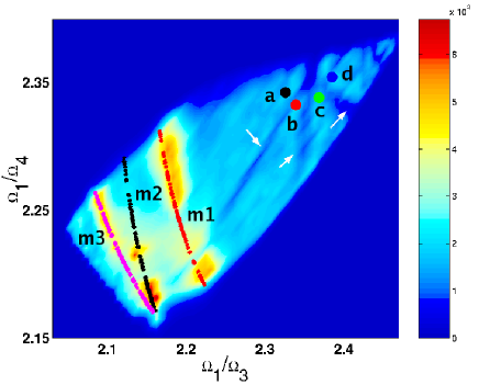
Figure 20: (Colour online) The dynamical Arnol’d web at $E=\bar{E}$ generated by propagating 25000 classical trajectories for $\tau\approx 40$. The primary resonances ${\bf m}_{1}$ (red), ${\bf m}_{2}$ (black), and ${\bf m}_{3}$ (magenta), as predicted by ${\cal H}_{0}$ are superimposed for comparison. The zeroth-order states of interest however are located far away from the primary resonances and close to the junction of three weak induced resonances ${\bf m}_{i1}=(0,0,1,-1),{\bf m}_{i2}=(0,1,-1,0)$, and ${\bf m}_{i3}=(0,1,0,-1)$ indicated by arrows. The induced resonances lead to the observed state mixings in Fig. 17 and Fig. 19 via the mechanism of RAT. The data for this figure were generated by A. Semparithi. Reproduced from ref. Kes051, .

How can one be sure that it is indeed the RAT mechanism that is at work here? The simplest answer is to try and interfere with the RAT mechanism by removing or alteringKes051 the relevant resonances as seen in Fig. 20. This was precisely what was done in the recent workKes051 and classical perturbation theory is again used to remove the primary resonances in Eq. (64) to $O(\epsilon)$. Since the methodology is well known only a brief description of the perturbative analysis follows. The first step involves reduction of the Hamiltonian in Eq. (64), noting the exactly conserved polyad $P_{c}$, to an effective three degrees of freedom system. This is achieved by performing a canonical transformation $({\bf I},{\bm{\theta}})\rightarrow({\bf J},{\bm{\psi}};P_{c})$ via the generating function

$$F({\bf J},{\bm{\psi}};P_{c})=\sum_{r}({\bf m}_{r}\cdot{\bm{\theta}})J_{r}+\theta_{1}P_{c}$$ (67)

The new variables can be obtained in terms of the old variables by using the generating function properties ${\bm{\psi}}=\partial_{\bf J}F$ and ${\bf I}=\partial_{\bm{\theta}}F$. The reduced Hamiltonian takes the form

$$H({\bf J},{\bm{\psi}};P_{c})=H_{0}({\bf J};P_{c})+\epsilon\sum_{r}K_{{\bf m}_{r}}g_{r}({\bf J};P_{c})\cos\psi_{r}$$ (68)

with $g_{r}({\bf J};P_{c})$ being determined from the functions $f_{r}({\bf I})$. The resonant angles are related to the original angle variables by $\psi_{r}={\bf m}_{r}\cdot{\bm{\theta}}$. The dynamical web in Fig. 20 clearly shows that the zeroth-order states of interest are far away from the primary resonances. Thus the three primary resonances are removed to $O(\epsilon)$ by making use of the generating function

$$G=\sum_{r}\psi_{r}\bar{J}_{r}+\epsilon\sum_{r}d_{r}(\bar{{\bf J}})\sin\psi_{r}$$ (69)

where the unknown functions $d_{r}(\bar{{\bf J}})$ are to be chosen such that the reduced Hamiltonian does not contain the primary resonances to $O(\epsilon)$. Using the standard generating function relations one obtains

$$J_{r} = \bar{J}_{r}+\epsilon d_{r}(\bar{{\bf J}})\cos\psi_{r}$$ (70)

$$\bar{\psi}_{r} = \psi_{r}+\epsilon\sum_{r^{\prime}}d_{rr^{\prime}}(\bar{{\bf J}})\sin\psi_{r^{\prime}}$$ (71)

with $r=1,2,3$ and $d_{rr^{\prime}}(\bar{{\bf J}})\equiv\partial d_{r}(\bar{{\bf J}})/\partial\bar{J}_{r^{\prime}}$. Writing the reduced Hamiltonian in terms of the variables $(\bar{{\bf J}},\bar{{\bm{\psi}}})$ and using the identities involving the Bessel functions ${\mathcal{J}}_{n}$

$$\cos(\epsilon a\sin b) = {\mathcal{J}}_{0}(\epsilon a)+2\sum_{l\geq 1}{\mathcal{J}}_{2l}(\epsilon a)\cos(2lb)$$ (72)

$$\sin(\epsilon a\sin b) = 2\sum_{l\geq 0}{\mathcal{J}}_{2l+1}\sin((2l+1)b)$$ (73)

one determines the choice for the unknown functions to be

$$d_{r}(\bar{{\bf J}})=-K_{{\bf m}_{r}}\frac{g_{r}(\bar{{\bf J}};P_{c})}{\bar{\Omega}_{r}}$$ (74)

Consequently, at $O(\epsilon^{2})$ the effective Hamiltonian

$${\cal H}(\bar{{\bf J}},\bar{{\bm{\psi}}};P_{c})\approx{\cal H}_{0}(\bar{{\bf J}};P_{c})+\epsilon^{2}{\cal H}_{2}(\bar{{\bf J}},\bar{{\bm{\psi}}};P_{c})$$ (75)

containing the induced resonances is obtained.

Following the procedure for RAT the induced resonances are approximated by pendulums. For example in the case of ${\bf m}_{i3}$ one obtains

$${\cal H}_{eff}^{(24)}=\frac{(K_{24}-K_{24}^{r})^{2}}{2M_{24}}+2V_{24}\cos(2\phi_{24})$$ (76)

with $K_{24}\sim 2I_{4}$ and $2\phi_{4}\sim(\theta_{2}-\theta_{4})$. The resonance center is $K_{24}^{r}$ and the effective coupling can now be expressed in terms of the conserved quantities $I_{3},P_{c}$, and $P_{24}=I_{2}+I_{4}$. Note that $P_{24}$ is the appropriate polyad for the induced resonance $\Omega_{2}$:$\Omega_{4}$=$1$:$1$. Thus it is possible to explicitly identify (cf. Eq. (76)) the barrier for dynamical tunneling in this three degrees of freedom case. Observe that the barrier is parametrized by an exact constant of the motion $P_{c}$ and two approximate constants of the motion $I_{3}$, and $P_{24}$. The effective couplings can be translated back to effective quantum strengths $\lambda_{\bf m}\approx V_{\bf m}/2$ quite easily. The perturbative analysis, for parameters relevant to Fig. 18, yields

$$\lambda_{{\bf m}_{i1}}\ll|\lambda_{{\bf m}_{i2}}|\approx|\lambda_{{\bf m}_{i3}}|=0.07K_{{\bf m}_{2}}$$ (77)

and thus the induced resonances are more than an order of magnitude smaller in strength as compared to the primary resonances. Based on the RAT theory it is possible to provide an explanation for the drastically different behaviour of state $|a\rangle$ when compared to the other three states as seen in Fig. 19. The state $|a\rangle$ is not symmetrically located, refering to the arguments following Eq. (38), with respect to $|b\rangle$ and thus, combined with the smallness of $\lambda_{{\bf m}_{i1}}$, does not show significant mixing.

Given that the key resonances and their strengths are known (cf. Eq. (77)) is it possible to interfere with the mixing between the states? In other words one is exploring the possibility of controlling the dynamical tunneling, a quantum phenomenon, by modifying the local phase space structures. Consider modifying the quantum Hamiltonian (based on classical information!) of Eq. (62) as follows:

$$H^{\prime}=H+|\lambda_{{\bf m}_{i2}}|(a_{2}^{\dagger}a_{3}+H.c.)+|\lambda_{{\bf m}_{i3}}|(a_{2}^{\dagger}a_{4}+H.c.)$$ (78)

In the above terms have been added to counter the induced resonances. Due to the weakness of the induced couplings quantities like mean level spacings, eigenvalue variations shown in Fig. 19, and spectral intensities show very little change as compared to the original system. However Fig. 21 shows that the survival probabilities of all the states exhibit long time trapping. The dilution factors shown in Fig. 21 also indicate almost no mixing between the near-degenerate states. Thus dynamical tunneling has been essentially shut down for these states. The fractionation pattern for the states with the modified Hamiltonian is quite similar to the ones seen in Fig. 19. One again observes a clump of off-resonant states around the same region. Surely the vibrational superexchange calculation would now predict the absence of mixing due to subtle cancellations but it is clear that a more transparent explanation comes from the RAT mechanism. More significantly Fig. 21 shows that other nearby zeorth-order states are unaffected by the counter resonant terms. Thus this is an example of local control of dynamical tunneling or equivalently IVR.

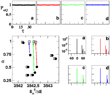
Figure 21: (Colour online) The top panel shows the survival probabilities for the states of interest using the modified Hamiltonian in Eq. (78). Note that the counter resonant terms have essentially shut off the dynamical tunneling proving the RAT mechanism. The bottom left figure shows the change in the dilution factors. Solid symbols refer to the $\sigma$ calculated from the original Hamiltonian in Eq. (62) (cf. Fig. 17C) and the open squares are the $\sigma$ calculated using Eq. (78). Only the states influenced by the induced resonances in Fig. 20 have their $\sigma\rightarrow 1$ whereas nearby states show very little change. The four panels on the right show the overlap intensity for the modified Hamiltonian. Notice the clump of states near $\approx 60\Delta E$ as in Fig. 19.

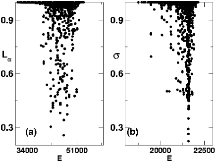
Figure 22: Additional examples for state mixings due to weak couplings. (a) Interpolyad mixing between the eigenstates of the Baggott Hamiltonian due to the polyad breaking Hamiltonian in Eq. (61) with $\delta=0.1$ cm^-1. The inverse participation ratios of the various eigenstates of $H_{3d}$ in the Baggott eigenbasis are shown versus the eigenvalues $E$ in cm^-1. (b) Dilution factors of the zeroth-order states for a Hamiltonian of the form as in Eq. (62) but with a different $H_{0}$. The polyad chosen is $P=16$ and the three resonant couplings have strengths $0.5K_{{\bf m}_{1}}=K_{{\bf m}_{2}}=K_{{\bf m}_{3}}\approx 0.05$ in units of the mean level spacing, $\Delta E\approx 1.8$ cm^-1. The zeroth-order energies $E$ are also in units of $\Delta E$.

The model Hamiltonian results in this section correspond to the near-integrable limit and thus RAT accounts for the state mixings. It would be interesting to study the mixed phase space limit for three degrees of freedom systems where classical transport mechanisms can compete as well. This however requires a careful study by varying the effective $\hbar$ of the system in order to distinguish between the classical and quantum mechanisms. Note that such zeroth-order state mixing due to weak couplings occurs in other model systems as well. In particular the present analysis and insight suggests that the mixing of edge and interior zeroth-order states in cyanoacetyleneHut84 must be due to the RAT mechanism. Two more examples in Fig. 22 highlight the mixing between near-degenerate states due to very weak couplings. The case in Fig. 22a corresponds to the mixings induced by the weak $3$:$1$ resonance in the case of the model Hamiltonian of Eq. (61) with $\delta=0.1$ cm^-1. The inverse participation ratios of the eigenstates $|\alpha_{3d}\rangle$ of $H_{3d}$

$$L_{\alpha}^{(3d)}\equiv\sum_{P}|\langle\alpha_{P}|\alpha_{3d}\rangle|^{4}$$ (79)

are calculated in the Baggott eigenbasis $\{|\alpha_{P}\rangle\}$ spanning several polyads centered about $P=16$. By construction the participation ratio of every eigenstate would be close to unity if the small $\delta$ value did not induce any interpolyad mixing. However it is clear from Fig. 22a that several eigenstates do get mixed. The other example shown in Fig. 22b pertains to a case where the Hamiltonian is of the same form as in Eq. (62) but with the parametrs of $H_{0}$ that corresponds to the CF₃CHFI moleculepqsw00 . The dilution factors of the various zeroth-order states in the polyad $P=16$ with extremely small couplings exhibit mixing. In both the examples it would be interesting to ascertain the percentage of states that are mixed due to CAT/RAT.

VI Summary

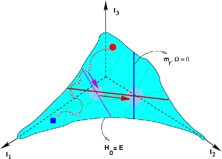
Figure 23: (Colour online) A sketch of the resonance web in three degrees of freedom in the $(I_{1},I_{2},I_{3})$ action (state) space. The energy surface $H_{0}=E$ is intersected by several resonances which form the web and control the IVR out of a state located on the energy surface. The strength of the resonances is indicated by the thickness and shaded regions highlight some of the resonance junctions. Mixing i.e., energy flow between the state on the top (red circle) and a far away state (blue square) is due to RAT, CAT (a possible tunneling sequence is shown by red arrows), classical across and along (thick arrows) transport. The competition between the tunneling and classical transport mechanism depends on the effective $\hbar$ of the system. Barriers to classical transport do exist and are expected to play an important rolemde87 but they have not been indicated in this simple sketch.

The central message of this review is that both classical and quantum routes to IVR are controlled by the network of nonlinear resonances. A simple sketch of IVR in state space via classical diffusion and dynamical tunneling is shown in Fig. 23 and should be contrasted with the sketch shown in Fig. 3. The vibrational superexchange picture of Fig. 3 explaining IVR through the participation of virtual off-resonant states is equivalent to the picture shown in Fig. 23 which explains IVR in terms of the Arnol’d web and states on the energy shell. Furthermore, as sketched in Fig. 23, a given zeroth-order state is always close to some nonlinear resonance or the other. Thus it becomes important to know the dynamically relevant regions of the web. Classically it is possible to drift along the resonance lines and come close to the junction where several resonances meet. At a junction the actions can move along an entirely different resonance line. In this fashion, loosely referred to as Arnol’d diffusionArno64 ; Viva84 ; Cin02 , the classical dynamics can lead to energy flow between a given point in Fig. 23 and another distant point. Arnol’d diffusion, however, is exponentially slow and its existence requires several constraints to be satisfied by the systemShur76 ; Lochasi . Therefore dynamical tunneling between two far removed points shown in Fig. 23 is expected to be more probable and faster than the classical Arnol’d diffusion. On the other hand, for generic Hamiltonian systems, a specific primary resonance will be intersected by infinitely many weaker (higher order than the primary) resonances but finitely many stronger resonances. The stronger resonances can lead to a characteristic cross-resonance diffusion near the resonance junction. The cross-resonance diffusion, in contrast to the Arnol’d diffusion, takes place on time scales much shorter than exponentialHallbook . In Fig. 23 one can imagine a scenario wherein a sequence of dynamical tunneling events finally lands up close to a resonance junction. Would the classical erratic motion near the junction interfere with the dynamical tunneling process? Is it then possible that an edge state might compete with an interior state due to CAT and/or RAT? Note that the four zeroth-order states in Fig. 20 are in fact close to one such resonance junction. The classical survival probabilities in Fig. 18 indicate some transport but further studies are required in order to characterize the classical transport. The issues involved are subtle since the competition between the coexisting classical and quantum routes has hardly been studied up until now and warrants further attention. Few of the studies that have been performedlw971 ; dim02 ; dim021 ; Tan02 to date suggest that quantum effects tend to localize the along-resonance diffusion on the web.

Nearly a decade ago Leitner and Wolynes analysedlw96 the Hamiltonian in Eq. (3) to understand the role of the vibrational superexchange at low energies. Within the state space approach it was argued that the superexchange mechanisms contribute significantly to the energy flow from the edge states to the interior of the state space. More importantly the superexchange contributions modify the IVR threshold as quantified by the transition parameter $T(E)$ defined in Eq. (10). From the phase space perspective as in Fig. 23 the direct and superexchange processes correspond to classical and quantum dynamical tunneling mechanisms respectively which are determined by the topology of the web. In contrast, note that the present studies on the model Hamiltonian in Eq. (62) actually shows dynamical tunneling at fairly high energies and between interior states in the state space. Further studies on such model systems would lead to better insights into the nature of $T(E)$. It would certainly be interesting to see if the criteria $T(E)\approx 1$ of Leitner and Wolynes is related to the criteria for efficient CAT and RAT in the phase space. Needless to say, such studies combined with the idea of local control demonstrated in the pevious section can provide important insights towards controlling IVR. The effective $\hbar$ is expected to play a central role in deciding the importance of various phase space structures. However intutive notions based entirely on this ‘geometrical’ criteria can be misleading. For instance, Gong and Brumer in their studiesgb05 on the modified kicked rotor found the quantum dynamics to be strongly influenced by regular islands in the phase space whose areas were at least an order of magnitude smaller than the effective Planck constant. Another example comes from the work by Sirko and Kochsko02 wherein it was observed that the ionization of bichromatically driven hydrogen atoms is mediated by nonlinear common resonancesHow91 with phase space areas of the order of the Planck constant. Further examples can be found in the recent studiesss07 ; Kes05 .

Although for large molecules the vibrational superexchange viewpoint is perhaps the only choice for computations, for a mechanistic understanding the phase space perspective is inevitable. Furthermore, as noted earlier, there exists ample evidence for the notion that even in large molecules the actual effective dimensionality of the IVR manifold in the state space is far less than the theoretical maximum of $(3N-6)$. Hence detailed classical-quantum correspondence studies of systems with three or four degrees of freedom can provide useful insights into the IVR processes in large molecules. At the same time a proper understanding of and including the effect of partial barriers into the theory of dynamical tunneling is necessary for further progress. Some hints to the delicate competition between quantum and classical transport through cantori can be found in the fairly detailed studies by Maitra and Hellermh00 on the dynamics generated by the whisker mapChi79 . Such studies are required to gain insights into the method of controlling quantum dynamics via suitable modifications of the local phase space structurescbcflvpfg04 ; hcu06 . Extending the local phase space control idea to systems with higher degrees of freedom poses a difficult challenge. If the sketch in Fig. 23 is reasonable then it suggests that the real origins of the hierarchical nature of IVR, due to both quantum and classical routes, is intricately tied to the geometry of the Arnol’d web. Significant efforts are needed to characterize the resonance web dynamically in order to have a clear understanding of how the specific features of the web influence the IVR. Recent worksKes051 ; sblkt06 ; sk06 ; bhc05 ; wbw04 ; sclu04 ; acp130 are beginning to focus on extracting such details in systems with three or more degrees of freedom which promises to provide valuable insights into the classical and quantum mechanisms of IVR in polyatomic molecules. Perhaps such an understanding would allow one to locally perturb specific regions of the resonance web and hence ultimately lead to control over the classical and quantum dynamics.

VII Acknowledgements

It is a pleasure to acknowledge several useful discussions with Arul Lakshminarayan and Peter Schlagheck on the topic of dynamical tunneling. I am grateful to Prof. Steve Wiggins for his hospitality at Bristol where parts of this review were written in addition to discussions on the wavelet technique. Financial support for the author’s research reported here came from the Department of Science and Technology and the Council for Scientific and Industrial Research, India.

References

- (1) For a fairly comprehensive review see, V. A. Benderskii, D. E. Makarov, and C. A. Wight, Adv. Chem. Phys. 88, Wiley-Interscience, NY (1994).
- (2) R. T. Lawton and M. S. Child, Mol. Phys. 37, 1799 (1979).
- (3) M. J. Davis and E. J. Heller, J. Chem. Phys. 75, 246 (1981).
- (4) W. G. Harter and C. W. Patterson, J. Chem. Phys. 80, 4241 (1984).
- (5) A. M. Ozorio de Almeida, J. Phys. Chem. 88, 6139 (1984).
- (6) See for example the article by M. V. Kuzmin and A. A. Stuchebrukhov in Laser Spectroscopy of Highly Vibrationally Excited Molecules, Ed. V. S. Letokhov, Adam Hilger, Bristol, 1989.
- (7) M. V. Berry and K. E. Mount, Rep. Prog. Phys. 35, 315 (1972).
- (8) W. H. Miller, Adv. Chem. Phys. 25, 69 (1974).
- (9) M. Wilkinson, Physica 21D, 341 (1986).
- (10) E. J. Heller, J. Phys. Chem. A 103, 10433 (1999).
- (11) G. C. Smith and S. C. Creagh, J. Phys. A: Math. Gen. 39, 8283 (2006).
- (12) E. J. Heller, Nature (London) 412, 33 (2001).
- (13) E. J. Heller, J. Phys. Chem. 99, 2625 (1995).
- (14) J. Zakrzewski, D. Delande, and A. Buchleitner, Phys. Rev. E 57, 1458 (1998).
- (15) A. Buchleitner, D. Delande, and J. Zakrzewski, Phys. Rep. 368, 409 (2002).
- (16) C. Dembowski, H.-D. Gräf, A. Heine, R. Hofferbert, H. Rehfeld, and A. Richter, Phys. Rev. Lett. 84, 867 (2000).
- (17) R. Hofferbert, H. Alt, C. Dembowski, H.-D. Gräf, H. L. Harney, A. Heine, H. Rehfeld, and A. Richter, Phys. Rev. E 71, 046201 (2005).
- (18) J. U. Nöckel and A. D. Stone, Nature (London) 385, 45 (1997).
- (19) W. K. Hensinger, H. Häffner, A. Browaeys, N. R. Heckenberg, K. Helmerson, C. McKenzie, G. J. Milburn, W. D. Phillips, S. L. Rolston, H. Rubinstein-Dunlop, and B. Upcroft, Nature (London) 412, 52 (2001).
- (20) D. A. Steck, W. H. Oskay, and M. G. Raizen, Science 293, 274 (2001).
- (21) J. P. Bird, R. Akis, D. K. Ferry, A. P. S. de Moura, Y. C. Lai, and K. M. Indlekofer, Rep. Prog. Phys. 66, 583 (2003).
- (22) K. Giese, H. Ushiyama, K. Takatsuka, and O. Kühn, J. Chem. Phys. 122, 124307 (2005).
- (23) K. K. Lehmann, G. Scoles, and B. H. Pate, Annu. Rev. Phys. Chem. 45, 241 (1994).
- (24) M. Gruebele and R. Bigwood, Int. Rev. Phys. Chem. 17, 91 (1998).
- (25) M. Gruebele, Adv. Chem. Phys. 114, 193 (2000).
- (26) R. Marquardt and M. Quack in Encyclopedia of Chemical Physics and Physical Chemistry I, Eds. J. H. Moore and N. D. Spencer (IOP, Bristol, 2001), pp. 897-936.
- (27) M. Gruebele and P. G. Wolynes, Acc. Chem. Res. 37, 261 (2004).
- (28) M. Gruebele, Theor. Chem. Acc. 109, 53 (2003).
- (29) A detailed discussion can be found in the book by T. Baer and W. L. Hase, Unimolecular Reaction Dynamics: Theory and Experiments, Oxford University Press, Oxford (1996).
- (30) S. Yu. Grebenshchikov, R. Schinke, and W. L. Hase in Comprehensive Chemical Kinetics, vol. 39, Unimolecular Kinetics, Part 1. The Reaction Step, Ed. N. J. B. Green (Elsevier, Amsterdam, 2003), Chapter 3 and references therein.
- (31) E. Fermi, J. Pasta, and S. Ulam, Los Alamos report LA-1940 (1955).
- (32) D. K. Campbell, P. Rosenau, and G. M. Zaslavsky, Chaos 15, 015101 (2005), and references therein.
- (33) D. J. Nesbitt and R. W. Field, J. Phys. Chem. 100, 12735 (1996).
- (34) J. C. Keske and B. H. Pate, Annu. Rev. Phys. Chem. 51, 323 (2000).
- (35) S. A. Rice, Adv. Chem. Phys. 47, 117 (1981).
- (36) T. Uzer, Phys. Rep. 199, 73 (1991).
- (37) G. S. Ezra, Adv. Class. Traj. Meth. 3, 35 (1998).
- (38) M. Gruebele, J. Phys.: Condens. Matter 16, R1057 (2004).
- (39) J. Assmann, M. Kling, B. Abel, Angew. Chem. Int. Ed. 42, 2226 (2003).
- (40) L. E. Fried and G. S. Ezra, J. Chem. Phys. 86, 6270 (1987).
- (41) M. E. Kellman, J. Chem. Phys. 93, 6630 (1990).
- (42) S. Tomsovic, Phys. Scr. T90, 162 (2001).
- (43) R. S. Mackay, J. D. Meiss, and I. C. Percival, Physica D 13, 55 (1984).
- (44) M. J. Davis, J. Chem. Phys. 83, 1016 (1985).
- (45) M. J. Davis and S. K. Gray, J. Chem. Phys. 84, 5389 (1986).
- (46) S. K. Gray and S. A. Rice, J. Chem. Phys. 86, 2020 (1987).
- (47) C. C. Marston and N. De Leon, J. Chem. Phys. 91, 3392 (1989).
- (48) R. T. Skodje and M. J. Davis, J. Chem. Phys. 88, 2429 (1988).
- (49) S. Wiggins, Physica D 44, 471 (1990).
- (50) R. E. Gillilan and G. S. Ezra, J. Chem. Phys. 94, 2648 (1991).
- (51) A. M. Ozorio de Almeida, N. De Leon, M. A. Mehta, and C. C. Marston, Physica D 46, 265 (1990).
- (52) S. K. Gray, S. A. Rice, and M. J. Davis, J. Phys. Chem. 90, 3470 (1986).
- (53) C. C. Martens, M. J. Davis, and G. S. Ezra, Chem. Phys. Lett. 142, 519 (1987).
- (54) S. H. Tersigni and S. A. Rice, Ber. Bunseges. Phys. Chem. 92, 227 (1988).
- (55) N. De Leon, M. A. Mehta, and R. Q. Topper, J. Chem. Phys. 94, 8310 (1991).
- (56) N. De Leon, J. Chem. Phys. 96, 285 (1991).
- (57) S. Wiggins, Normally Hyperbolic Invariant Manifolds in Dynamical Systems, Springer Verlag, Berlin, 1994.
- (58) S. Wiggins, L. Wiesenfeld, C. Jaffé, and T. Uzer, Phys. Rev. Lett. 86, 5478 (2001).
- (59) T. Uzer, C. Jaffé, J. Palacian, P. Yanguas, and S. Wiggins, Nonlinearity 15, 957 (2002).
- (60) H. Waalkens, A. Burbanks, and S. Wiggins, J. Chem. Phys. 121, 1 (2004).
- (61) E. Shchekinova, C. Chandre, Y. Lan, and T. Uzer, J. Chem. Phys. 121, 3471 (2004).
- (62) See the contributions to, Geometric Structures of Phase Space in Multidimensional Chaos, Adv. Chem. Phys. 130, Eds. M. Toda, T. Komatsuzaki, T. Konishi, and R. S. Berry, Wiley-Interscience NY, (2005).
- (63) A. Bach, J. M. Hostettler, and P. Chen, J. Chem. Phys. 123, 021101 (2005).
- (64) H. Waalkens, A. Burbanks, and S. Wiggins, Phys. Rev. Lett. 95, 084301 (2005).
- (65) F. Gabern, W. S. Koon, J. E. Marsden, and S. D. Ross, Physica D 211, 391 (2005).
- (66) A. Bach, J. M. Hostettler, and P. Chen, J. Chem. Phys. 125, 024304 (2006).
- (67) A. Shojiguchi, A. Baba, C. B. Li, T. Komatsuzaki, and M. Toda, Laser Physics 16, 1097 (2006).
- (68) A. Semparithi and S. Keshavamurthy, J. Chem. Phys. 125, 141101 (2006).
- (69) A. Shojiguchi, C. B. Li, T. Komatsuzaki, and M. Toda, Phys. Rev. E 75, 035204(R) (2007).
- (70) H. Lefebvre-Brion and R. W. Field, The Spectra and Dynamics of Diatomic Molecules, Elsevier, NY, 2004.
- (71) D. Papousek and M. R. Aliev, Molecular Vibrational-Rotational Spectra, Elsevier, Amsterdam, 1982.
- (72) H. Ishikawa, R. W. Field, S. C. Farantos, M. Joyeux, J. Koput, C. Beck, and R. Schinke, Annu. Rev. Phys. Chem. 50, 443 (1999).
- (73) M. P. Jacobson and R. W. Field, J. Phys. Chem. A 104, 3073 (2000).
- (74) C. Jaffé and P. Brumer, J. Chem. Phys. 73, 5646 (1980).
- (75) M. E. Kellman and V. Tyng, Acc. Chem. Res. 40, 243 (2007).
- (76) J. H. Van Vleck, Rev. Mod. Phys. 23, 213 (1951).
- (77) M. Joyeux and D. Sugny, Can. J. Phys. 80, 1459 (2002).
- (78) A. B. McCoy and E. L. Sibert in Computational Molecular Spectroscopy, Eds. P. Jensen and P. R. Bunker, Wiley, Chichester (UK), 2000.
- (79) J. L. Dunham, Phys. Rev. 41, 721 (1932).
- (80) A. Callegari, H. K. Srivatsava, U. Merker, K. K. Lehmann, G. Scoles, and M. J. Davis, J. Chem. Phys. 106, 432 (1997).
- (81) S. A. Schofield and P. G. Wolynes, J. Chem. Phys. 98, 1123 (1992).
- (82) S. A. Schofield and P. G. Wolynes, J. Phys. Chem. 99, 2753 (1995).
- (83) S. A. Schofield, P. G. Wolynes, and R. E. Wyatt, Phys. Rev. Lett. 74, 3720 (1995).
- (84) S. A. Schofield, R. E. Wyatt, and P. G. Wolynes, J. Chem. Phys. 105, 940 (1996).
- (85) V. Wong and M. Gruebele, J. Phys. Chem. A 103, 10083 (1999).
- (86) D. E. Logan and P. G. Wolynes, J. Chem. Phys. 93, 4994 (1990).
- (87) D. M. Leitner and P. G. Wolynes, J. Chem. Phys. 105, 11226 (1996).
- (88) D. M. Leitner and P. G. Wolynes, J. Phys. Chem. A 101, 541 (1997).
- (89) T. A. Holme and J. S. Hutchinson, J. Chem. Phys. 84, 5455 (1986).
- (90) J. S. Hutchinson, Adv. Chem. Phys. LXXIII, 637 (1989).
- (91) E. R. Th. Kerstel, K. K. Lehmann, T. F. Mentel, B. H. Pate, and G. Scoles, J. Phys. Chem. 95, 8282 (1991).
- (92) J. E. Gambogi, J. H. Timmermans, K. K. Lehmann, and G. Scoles, J. Chem. Phys. 99, 9314 (1993).
- (93) J. E. Gambogi, R. L’Esperance, K. K. Lehmann, and G. Scoles, J. Phys. Chem. 98, 5614 (1994).
- (94) B. R. Foy, M. P. Casassa, J. C. Stephenson, and D. S. King, J. Chem. Phys. 89, 608 (1988).
- (95) A. McIlroy and D. J. Nesbitt, J. Chem. Phys. 91, 104 (1989).
- (96) J. Go and D. S. Perry, J. Chem. Phys. 97, 6994 (1992).
- (97) S. W. Mork, C. C. Miller, and L. A. Phillips, J. Chem. Phys. 97, 2971 (1992).
- (98) A. L. Utz, E. Carrasquillo, J. D. Tobiason, and F. F. Crim, Chem. Phys. 190, 311 (1995).
- (99) A. Callegari, R. Pearman, S. Choi, P. Engels, H. Srivastava, M. Gruebele, K. K. Lehmann, and G. Scoles, Mol. Phys. 101, 551 (2003).
- (100) A. Portnov, S. Rosenwaks, and I. Bar, J. Chem. Phys. 121, 5860 (2004).
- (101) O. V. Boyarkin and T. R. Rizzo, J. Chem. Phys. 105, 6285 (1996).
- (102) L. Lubich, O. V. Boyarkin, R. D. F. Settle, D. S. Perry, and T. R. Rizzo, Farad. Disc. 102, 167 (1996).
- (103) A. A. Stuchebrukhov and R. A. Marcus, J. Chem. Phys. 98, 6044 (1993).
- (104) J. S. Hutchinson, E. L. Sibert III, and J. T. Hynes, J. Chem. Phys. 81, 1314 (1984).
- (105) A. A. Stuchebrukhov and R. A. Marcus, J. Chem. Phys. 98, 8443 (1993).
- (106) J. S. Hutchinson, J. Chem. Phys. 82, 22 (1984).
- (107) R. T. Lawton and M. S. Child, Mol. Phys. 40, 773 (1980).
- (108) R. T. Lawton and M. S. Child, Mol. Phys. 44, 709 (1981).
- (109) M. S. Child and R. T. Lawton, Chem. Phys. Lett. 87, 217 (1982).
- (110) L. Halonen, Adv. Chem. Phys. 104, 41 (1998).
- (111) P. Jensen, Mol. Phys. 98, 1253 (2000).
- (112) B. R. Henry and H. G. Kjaergaard, Can. J. Chem. 80, 1635 (2002).
- (113) E. J. Heller, E. B. Stechel, and M. J. Davis, J. Chem. Phys. 73, 4720 (1980).
- (114) E. J. Heller and M. J. Davis, J. Phys. Chem. 85, 307 (1981).
- (115) M. J. Davis and E. J. Heller, J. Chem. Phys. 80, 5036 (1984).
- (116) E. L. Sibert III, W. P. Reinhardt, and J. T. Hynes, J. Chem. Phys. 77, 3583 (1982).
- (117) E. L. Sibert III, J. T. Hynes, and W. P. Reinhardt, J. Chem. Phys. 77, 3595 (1982).
- (118) W. G. Harter, J. Chem. Phys. 85, 5560 (1986).
- (119) E. L. Sibert III, J. Chem. Phys. 83, 5092 (1985).
- (120) K. Stefanski and E. Pollak, J. Chem. Phys. 87, 1079 (1987).
- (121) M. E. Kellman, J. Phys. Chem. 87, 2161 (1982).
- (122) P. R. Bunker and P. Jensen, Molecular Symmetry and Spectroscopy, 2nd ed. NRC research press, Ottawa (1998).
- (123) D. Babyuk, R. E. Wyatt, and J. H. Frederick, J. Chem. Phys. 119, 6482 (2003).
- (124) J. S. Go, T. J. Cronin, and D. S. Perry, Chem. Phys. 175, 127 (1993).
- (125) A. A. Stuchebrukhov, A. Mehta, and R. A. Marcus, J. Phys. Chem. 97, 12491 (1993).
- (126) A. Mehta, A. A. Stuchebrukhov, and R. A. Marcus, J. Phys. Chem. 99, 2677 (1995).
- (127) M. D. Newton, Chem. Rev. 91, 767 (1991).
- (128) P. Siddarth and R. A. Marcus, J. Phys. Chem. 96, 3213 (1992).
- (129) R. Pearman and M. Gruebele, J. Chem. Phys. 108, 6561 (1998).
- (130) W. A. Lin and L. E. Ballentine, Phys. Rev. Lett. 65, 2927 (1990).
- (131) W. A. Lin and L. E. Ballentine, Phys. Rev. A 45, 3637 (1992).
- (132) A. Peres, Phys. Rev. Lett. 67, 158 (1991).
- (133) W. A. Lin and L. E. Ballentine, Phys. Rev. Lett. 67, 159 (1991).
- (134) F. Grossmann, T. Dittrich, P. Jung, and P. Hänggi, Phys. Rev. Lett. 67, 516 (1991).
- (135) J. M. G. Llorente and J. Plata, Phys. Rev. A 45, R6958 (1992).
- (136) R. Utermann, T. Dittrich, and P. Hänggi, Phys. Rev. E 49, 273 (1994).
- (137) D. Farrelly and J. A. Milligan, Phys. Rev. E 47, R2225 (1993).
- (138) M. Latka, P. Grigolini, and B. J. West, Phys. Rev. A 50, 1071 (1994).
- (139) V. Averbukh, N. Moiseyev, B. Mirbach, and H. J. Korsch, Z. Phys. D 35, 247 (1995).
- (140) M. E. Flatté and M. Holthaus, Ann. Phys. (N. Y.) 245, 113 (1996).
- (141) E. M. Zanardi and J. M. G. Llorente, Chem. Phys. 217, 221 (1997).
- (142) A. Mouchet, C. Miniatura, R. Kaiser, B. Gremaud, and D. Delande, Phys. Rev. E 64, 016221 (2001).
- (143) S. Osovski and N. Moiseyev, Phys. Rev. A 72, 033603 (2005).
- (144) R. Grobe and F. Haake, Z. Phys. B 68, 503 (1987).
- (145) M. Grifoni and P. Hänggi, Phys. Rep. 304, 229 (1998).
- (146) J. Gong and P. Brumer, Annu. Rev. Phys. Chem. 56, 1 (2005).
- (147) O. Bohigas, S. Tomsovic, and D. Ullmo, Phys. Rep. 223, 43 (1993).
- (148) S. Tomsovic and D. Ullmo, Phys. Rev. E 50, 145 (1994).
- (149) O. Bohigas, D. Boosé, R. Eygdio de Carvalho, and V. Marvulle, Nucl. Phys. A 560, 197 (1993).
- (150) E. Doron and S. D. Frischat, Phys. Rev. Lett. 75, 3661 (1995).
- (151) S. D. Frischat and E. Doron, Phys. Rev. E 57, 1421 (1998).
- (152) F. Leyvraz and D. Ullmo, J. Phys. A: Math. Gen. 29, 2529 (1996).
- (153) S. C. Creagh, J. Phys. A: Math. Gen. 27, 4969 (1994).
- (154) S. C. Creagh and N. D. Whelan, Phys. Rev. Lett. 84, 4084 (2000).
- (155) S. C. Creagh and N. D. Whelan, Phys. Rev. Lett. 77, 4975 (1996).
- (156) S. C. Creagh and N. D. Whelan, Ann. Phys. (N. Y.) 272, 196 (1999).
- (157) S. C. Creagh in Tunneling in Complex Systems, edited by S. Tomsovic, page 35-100, World Scientific, NJ, 1998.
- (158) A. Mouchet and D. Delande, Phys. Rev. E 67, 046216 (2003).
- (159) R. Egydio de Carvalho and A. P. Mijolaro, Phys. Rev. E 70, 056212 (2004).
- (160) V. A. Podolskiy and E. E. Narimanov, Phys. Rev. Lett. 91, 263601 (2003).
- (161) V. A. Podolskiy and E. E. Narimanov, Opt. Lett. 30, 474 (2005).
- (162) R. Roncaglia, L. Bonci, F. M. Izrailev, B. J. West, and P. Grigolini, Phys. Rev. Lett. 73, 802 (1994).
- (163) T. Geisel, G. Radons, and J. Rubner, Phys. Rev. Lett. 57, 2883 (1986).
- (164) G. Radons, T. Geisel, and J. Rubner, Adv. Chem. Phys. LXXIII, 891 (1989).
- (165) R. Ketzmerick, L. Hufnagel, F. Steinbach, and M. Weiss, Phys. Rev. Lett. 85, 1214 (2000).
- (166) G. Radons and R. E. Prange, Phys. Rev. Lett. 61, 1691 (1988).
- (167) N. T. Maitra and E. J. Heller, Phys. Rev. E 61, 3620 (2000).
- (168) A. Shudo and K. S. Ikeda, Phys. Rev. Lett. 74, 682 (1995).
- (169) A. Shudo and K. S. Ikeda, Phys. Rev. Lett. 76, 4151 (1996).
- (170) A. Shudo and K. S. Ikeda, Physica 115D, 234 (1998).
- (171) T. Onishi, A. Shudo, K. S. Ikeda, and K. Takahashi, Phys. Rev. E 64, 025201 (2001).
- (172) A. Shudo, Y. Ishii, and K. S. Ikeda, J. Phys. A: Math. Gen. 35, L225 (2002).
- (173) K. Takahashi and K. S. Ikeda, J. Phys. A: Math. Gen. 36, 7953 (2003).
- (174) K. Takahashi and K. S. Ikeda, Europhys. Lett. 71, 193 (2005).
- (175) N. Hashimoto and K. Takatsuka, J. Chem. Phys. 108, 1893 (1997).
- (176) O. Brodier, P. Schlagheck, and D. Ullmo, Phys. Rev. Lett. 87, 064101 (2001).
- (177) O. Brodier, P. Schlagheck, and D. Ullmo, Ann. Phys. (N. Y.) 300, 88 (2002).
- (178) P. Schlagheck, C. Eltschka, and D. Ullmo in Progress in Ultrafast Intense Laser Science I, Eds. K. Yamanouchi, S. L. Chin, P. Agostini, and G. Ferrante (Springer, Berlin, 2006), pp. 107-131.
- (179) P. Schlagheck, Tunneling in the presence of chaos and interactions, Habilitationsschrift, Universität Regensburg, 2006.
- (180) A. J. Lichtenberg and M. A. Lieberman, Regular and Stochastic Motion, Springer-Verlag, NY (1983).
- (181) S. Takada, P. N. Walker, and M. Wilkinson, Phys. Rev. A 52, 3546 (1995).
- (182) C. Eltschka and P. Schlagheck, Phys. Rev. Lett. 94, 014101 (2005).
- (183) S. Wimberger, P. Schlagheck, C. Eltschka, and A. Buchleitner, Phys. Rev. Lett. 97, 043001 (2006).
- (184) A. Mouchet, C. Eltschka, and P. Schlagheck, Phys. Rev. E 74, 026211 (2006).
- (185) M. Sheinman, S. Fishman, I. Guarneri, and L. Rebuzzini, Phys. Rev. A 73, 052110 (2006).
- (186) A. Sethi and S. Keshavamurthy, manuscript in preparation,2007.
- (187) J. Feist, A. Bäcker, R. Ketzmerick, S. Rotter, B. Huckestein, and J. Burgdörfer, Phys. Rev. Lett. 97, 116804 (2006).
- (188) M. Sheinman, Decay of Quantum Accelarator Modes, Master’s thesis, Chapter 3, Technion, 2005.
- (189) R. C. Brown and R. E. Wyatt, Phys. Rev. Lett. 57, 1 (1986).
- (190) R. C. Brown and R. E. Wyatt, J. Phys. Chem. 90, 3590 (1986).
- (191) Recent work from the group of P. Schlagheck has managed to include the cantorus structure into the framework of RAT and substantial improvements are seen between semiclassical and quantum results for the splittings in the kicked Harper model. (Private communication).
- (192) A. Nitzan, Annu. Rev. Phys. Chem. 52, 681 (2001).
- (193) S. Flach, V. Fleurov, and A. A. Ovchinnikov, Phys. Rev. B 63, 094304 (2001).
- (194) J. Dorignac and S. Flach, Phys. Rev. B 65, 214305 (2002).
- (195) R. A. Pinto and S. Flach, Phys. Rev. A 73, 022717 (2006).
- (196) V. Fleurov, Chaos 13, 676 (2003).
- (197) S. Flach and V. Fleurov, J. Phys.: Condens. Matter 9, 7039 (1997).
- (198) D. K. Campbell, S. Flach, and Y. S. Kivshar, Phys. Today 57, 43 (2004).
- (199) J. Dorignac, J. C. Eilbeck, M. Salerno, and A. C. Scott, Phys. Rev. Lett. 93, 025504 (2004).
- (200) J. E. Baggott, Mol. Phys. 65, 739 (1988).
- (201) J. Tennyson, N. F. Zobov, R. Williamson, O. L. Polyansky, and P. F. Bernath, J. Phys. Chem. Ref. Data 30, 735 (2001).
- (202) S. Keshavamurthy and G. S. Ezra, Chem. Phys. Lett. 259, 81 (1995).
- (203) S. Keshavamurthy and G. S. Ezra, J. Chem. Phys. 107, 156 (1997).
- (204) Z. M. Lu and M. E. Kellman, J. Chem. Phys. 107, 1 (1997).
- (205) S. Keshavamurthy, J. Chem. Phys. 119, 161 (2003).
- (206) S. Keshavamurthy, J. Chem. Phys. 122, 114109 (2005).
- (207) B. V. Chirikov, Phys. Rep. 52, 263 (1979).
- (208) We note here a typographical error in Eq.(19a) of ref. Kes05, involving the expression for . The corrected version appears in this review as Eq. (58c).
- (209) M. P. Jacobson, C. Jung, H. S. Taylor, and R. W. Field, J. Chem. Phys. 111, 600 (1999).
- (210) J. Keske, D. A. McWhorter, and B. H. Pate, Int. Rev. Phys. Chem. 19, 363 (2000).
- (211) K. K. Lehmann, J. Chem. Phys. 95, 2361 (1991).
- (212) K. K. Lehmann, J. Chem. Phys. 96, 7402 (1992).
- (213) M. S. Child and Q. Zhu, Chem. Phys. Lett. 184, 41 (1991).
- (214) H. P. Breuer and M. Holthaus, J. Phys. Chem. 97, 12634 (1993).
- (215) D. M. Leitner and P. G. Wolynes, Phys. Rev. Lett. 76, 216 (1996).
- (216) J. Ortigoso, Phys. Rev. A 54, R2521 (1996).
- (217) L. Bonci, A. Farusi, P. Grigolini, and R. Roncaglia, Phys. Rev. E 58, 5689 (1998).
- (218) S. Tomsovic, J. Phys. A: Math. Gen. 31, 9469 (1998).
- (219) Y. Ashkenazy, L. Bonci, J. Levitan, and R. Roncaglia, Phys. Rev. E 64, 056215 (2001).
- (220) S. Keshavamurthy, Phys. Rev. E 72, 045203(R) (2005).
- (221) A. Beil, H. Hollenstein, O. L. A. Monti, M. Quack, and J. Stohner, J. Chem. Phys. 113, 2701 (2000).
- (222) M. Carioli, E. J. Heller, and K. B. Moller, J. Chem. Phys. 106, 8564 (1997).
- (223) J. Laskar, Physica D 67, 257 (1993).
- (224) J. v. Milczewski, G. H. F. Diercksen, and T. Uzer, Phys. Rev. Lett. 76, 2890 (1996).
- (225) J. V. Vela-Arevalo and S. Wiggins, Int. J. Bifur. Chaos. 11, 1359 (2001).
- (226) C. Chandre, S. Wiggins, and T. Uzer, Physics D 181, 171 (2003).
- (227) J. Pochert, M. Quack, J. Stohner, and M. Willeke, J. Chem. Phys. 113, 2719 (2000).
- (228) V. I. Arnol’d, Sov. Math. Dokl. 5, 581 (1964).
- (229) F. Vivaldi, Rev. Mod. Phys. 56, 737 (1984).
- (230) P. M. Cincotta, New. Aston. Rev. 46, 13 (2002).
- (231) E. V. Shuryak, Sov. Phys. JETP 44, 1070 (1976).
- (232) P. Lochak, Hamiltonian Systems with Three or More Degrees of Freedom, Ed. C. Simo, NATO ASI 533, (Kluwer, Boston, 1999), pp. 168-183.
- (233) G. Haller, Chaos Near Resonance, (Springer, Berlin, 1999).
- (234) D. M. Leitner and P. G. Wolynes, Phys. Rev. Lett. 79, 55 (1997).
- (235) V. Ya. Demikhovskii, F. M. Izrailev, and A. I. Malyshev, Phys. Rev. Lett. 88, 154101 (2002).
- (236) V. Ya. Demikhovskii, F. M. Izrailev, and A. I. Malyshev, Phys. Rev. E 66, 036211 (2002).
- (237) E. Tannenbaum, Ph.D thesis, Harvard University, chapter 3, 2002.
- (238) L. Sirko and P. M. Koch, Phys. Rev. Lett. 89, 274101 (2002).
- (239) J. E. Howard, Phys. Lett. A 156, 286 (1991).
- (240) G. Ciraolo, F. Briolle, C. Chandre, E. Floriani, R. Lima, M. Vittot, C. Figarella, and P. Ghendrih, Phys. Rev. E 69, 056213 (2004).
- (241) S. Huang, C. Chandre, and T. Uzer, Phys. Rev. A 74, 053408 (2006).