Heat Transfer in Underground Rail Tunnels

Abstract

The transfer of heat between the air and surrounding soil in underground tunnels ins investigated, as part of the analysis of environmental conditions in underground rail systems. Using standard turbulent modelling assumptions, flow profiles are obtained in both open tunnels and in the annulus between a tunnel wall and a moving train, from which the heat transfer coefficient between the air and tunnel wall is computed. The radial conduction of heat through the surrounding soil resulting from changes in the temperature of air in the tunnel are determined. An impulse change and an oscillating tunnel air temperature are considered separately. The correlations between fluctuations in heat transfer coefficient and air temperature are found to increase the mean soil temperature. Finally, a model for the coupled evolution of the air and surrounding soil temperature along a tunnel of finite length is given.

1 Introduction

Aero-thermodynamic analysis of the environmental conditions within underground tunnels has a number of engineering applications. Perhaps the most widespread application involves modelling the air temperatures and conditions expected in underground rail stations. The paper by Abi-Zadeh et al. (2003) is one example of many publications on this subject: there the air temperature within London’s King’s Cross Underground Station was simulated and compared with measurements taken within the existing station in order to validate the model. The model was then changed to reflect proposed modifications to the station and re-run to simulate future conditions. The main aim was to ensure that overheating of the station does not occur as a result of increased patronage and servicing.

The software used to develop such models must simulate a large number of phenomena. Typically, an aerodynamic network model of the tunnels, stations, passageways and ventilation shafts is the basis of the model and is used to predict air movements generated by trains moving through the system. The heat generated and released by trains (by far the largest source of heat energy within an underground rail system) is typically also computed. The effect of other heat sources such as electro-mechanical equipment, lighting and passengers is accounted for.

The final factor, which cannot be accounted for by a steady-state heat balance approach, is the thermal interaction between air within the tunnel and the surrounding soil. The tunnel lining and surrounding soil have a large thermal mass and are strongly coupled to the air within the system, so they must be included if conditions in the underground environment are to be accurately modelled. However, as we will show, the effect of the surrounding soil depends on a large number of parameters, including the magnitude and frequency of fluctuations in ambient air temperature due to daily and seasonal oscillations.

Details of a comprehensive thermal model of an underground railway environment are given by Ampofo et al. (2004). Results presented in their paper give an overview of the relative importance of heat loads and sinks within an underground system. For instance, during peak summer conditions 85% of the heat load in a tunnel is generated by train braking systems, 13% by other systems on the trains and 2% from tunnel lighting and other loads within the tunnels. Hence, the introduction of regenerative braking systems has the greatest potential to reduce the total thermal load and hence peak temperatures. The model also predicts that 70% of the heat load is removed by air moving through the tunnels and the remaining 30% is lost by conduction into the tunnel walls. However, the thermal model treats the tunnel wall as a thermal resistance only, and hence does not take into account the thermal mass of the tunnel walls and surrounding soil. As a result the daily and seasonal phase shift in tunnel air temperatures observed by Abi-Zadeh et al. (2003)—the fact that the Underground warms up over the summer and is therefore warmer in autumn than spring for the same ambient conditions—cannot be predicted by ther model. From a more practical point of view, this limitation also means that standard steady-state modelling cannot predict what effect ‘night flushing’—using fans to move cool night air through the tunnels when trains are not operating—will have on the peak temperature in the tunnels the next day. It is these effects that we address in this paper.

Our analysis encompasses the following effects:

• Section 2 – Turbulent flow profiles. We present analytic formulations of the turbulent flow profiles expected in both an open tunnel and in the annulus between the tunnel and a passing train are presented. These are used to compute the coefficient governing heat transfer between the air and the internal surface of the tunnel.

• Sections 3 and 4 – Radial heat conduction. Using the flow profiles above, we derive analytic solutions governing the radial conduction of heat in a cylindrical coodinate system. The conducting domain extends from an internal radius to infinity. Heat transfer into the solid from the internal radius is conductive and proportional to the difference between the temperature of the air within the tunnel and the temperature at the wall surface.

• Section 5 – Short-term fluctuations. We consider the effect of short-term fluctuations in heat transfer coefficient caused by the passage of trains. The approach currently used in engineering calculations involves time averaging the heat transfer coefficient over the short-term fluctuations. A more comprehensive approach, not currently used, is presented, involving the correlation between short-term fluctuations in heat transfer coefficient and tunnel air temperature, both caused by passing trains. We show that such a correlation manifests itself as an additional heat source within the tunnel and hence raises the mean temperature.

• Section 6 – Coupled evolution of air and soil temperatures. Finally, we present a model for the coupled evolution of air temperature (along the axis of a tunnel) and soil (radially from the tunnel surface). Unlike previous models, such as Peavy (1961) this accounts for a continuous inhomogeneous heat source along the tunnel axis.

To give the reader a feel for the magnitude of the effects involved, we use specific values for physical parameteres throughout the paper. Unless otherwise stated, we use parameters typical of London’s Piccadilly line tunnels and trains. For easy reference, these parameter values are documented in tables in Appendix A.

2 Heat Transfer Coefficient at the Tunnel Wall

In its most fundamental form, the problem under consideration is described by Newton’s law of cooling: the heat flux between the air within a tunnel and the surrounding soil is proportional to the difference between the temperature of the air and of the tunnel wall surface. The magnitude of the heat transfer or flux for a given temperature difference is dictated by the heat transfer coefficient $h$, a parameter that is a function of the nature of the air flow and properties of the wall surface.

In this section we present mathematical approximations of steady state (time independent) air flow through a train tunnel. As per previous work on this subject by Barrow and Pope (1987) and Shigechi et al. (1990), we consider two distinct cases. Firstly, air flow through a circular tunnel, and secondly, air flow in the annulus between a stationary circular tunnel and a concentric circular core moving in the axial direction. These two cases represent, respectively, air flow through an open tunnel and in the annulus between a tunnel wall and moving train. In both cases we show that the flows are fully turbulent under the generic conditions considered, and give generic turbulent flow profiles.

We then use the so-called ‘Reynolds analogy’ to relate the air flow velocity profile, as described above, to the air flow temperature profile. This analogy gives an approximation to the heat transfer coefficient $h$ as a function of the flow shear stress at the tunnel wall $\tau_{w}$. As a result, the heat transfer coefficient can be estimated from the parameters of the air flows through the tunnel and through the annulus between the tunnel wall and a passing train.

2.1 Turbulent Flow Through an Unobstructed Tunnel

As mentioned above, the tunnel air flow profile, and hence the heat transfer coefficient, is drastically different depending on its regime, which can be laminar, turbulent, or intermediate between the two. The regime is determined using the dimensionless Reynolds number. For flow in a circular pipe, or in this case tunnel, the Reynolds number is defined by Schlichting and Gersten (2000, Eq. 17.129) as $Re={U_{t}a}/{\nu}$. Here, in cylindrical polar coordinates, $U_{t}$ is the mean fluid velocity along the axis of the pipe for a flow $u(r)$, $a$ is the radius of the pipe wall, and $\nu$ is the kinematic viscosity of the fluid.

In general, flow with this geometry is fully turbulent if $Re>2000$, as can be shown on a Moody diagram (Kreith and Bohn, 1993, Figure 6.8). For a typical air flow through a tunnel induced by train piston effect, $Re\approx 10^{6}$—the flow is assumed to be fully turbulent. This means that the flow will not be uni-directional, and hence the well-known Poiseuille solution where the radial velocity distribution is parabolic does not apply. We must resort to turbulent modeling of the mean flow profile. Here we will use Prandtl’s mixing length hypothesis, which gives a mean velocity distribution as a logarithmic profile from the tunnel wall, and symmetrical about the centre of the tunnel ($r=0$). This is discussed in numerous texts on turbulent flow, for instance Pope (2001).

A generic mean velocity profile for fully turbulent flow in a pipe or radius $a$ is

$${u(y)}/{v_{*}}=2.5\log{\left({y}/{k}\right)}+8.5\,,$$ (1)

for $0\leq y\leq a$ where $y=a-r$, the distance into the flow from the wall boundary and $k$ is the roughness length of the wall surface. Further,

$$v_{*}=\sqrt{\tau/\rho}$$ (2)

is the friction velocity where $\tau$ is the turbulent shear stress of the flow, a constant over the diameter of the pipe, and $\rho$ is the density of the fluid.

It should be noted that in (1), the constant term given as $8.5$ is in fact a parameter of the flow. The value given applies to flow over a ‘rough’ wall, which requires $v_{*}k/\nu>70$, which we will show is the case for the parameters under consideration. For flow over a ‘smooth’ wall, which is indicated by $v_{*}k/\nu<70$, the constant term becomes a function of the roughness parameter as described fox example in Grimson (1971).

Although the generic velocity profile takes the form of (1), a specific friction velocity must be calculated for a particular flow. This will then define the velocity profile across the pipe and hence the wall shear stress by (2). We are presuming the flux, produced by either the train piston effect or a ventilation system, is known. This value will normally be provided by either measurements or aerodynamic modelling.

The flow rate down the tunnel, $Q$, can also be related to the mean flow profile, $u(r)$, as

$$Q=2\pi\int_{0}^{a}{ru(r)dr}\,.$$ (3)

When combined with (1), this provides the relationship

$$v_{*}=\frac{Q}{2\pi a^{2}\left(2.375+1.25\log\left(1/k\right)\right)}$$ (4)

for the friction velocity.

Figure 1: Tunnel flow profile using the Piccadilly line parameters.

We have used parameters for a typical tunnel section of the Piccadilly line to generate a flow profile using (1) and (4). The fully developed mean flow profile, $\bar{u}(r)$, is shown in Figure 1. The values assumed for the various parameters and related calculations are presented in Appendix A. The Reynolds number of the flow is approximately $10^{6}$. The shear stress at the tunnel wall for flow in the annulus, $\tau_{w}$ is approximately $0.44$ N/m². The flow number, $v_{*}k/\nu$, is equal to 392, so the assumption that the wall is rough can be made.

2.2 Turbulent Flow in the Train–Tunnel Annulus

The velocity profile adjacent to the tunnel wall changes considerably as a train passes, which affects the heat transfer between the air and the wall. In this section the air flow in the gap between the outer surface of a train and the tunnel wall is considered. This flow is approximated by treating the train as a circular core moving concentrically through the circular tunnel as per the approach by Barrow and Pope (1987) and Shigechi et al. (1990). The radius of the central core, $b$, is then calculated by equating the frontal area of the train and the cross section of the cylindrical core. The Reynolds number for flow in such an annulus is defined by Shigechi et al. (1990) as

$$Re_{a}=\frac{2U_{a}(a-b)}{\nu}.$$ (5)

2.3 Generic Annulus Velocity Profile

The general strategy for determining the flow profile through the tunnel–train annulus, as outlined in Barrow and Pope (1987) is to match two boundary layers of the form given by (1). This is shown diagramatically in Figure 2.

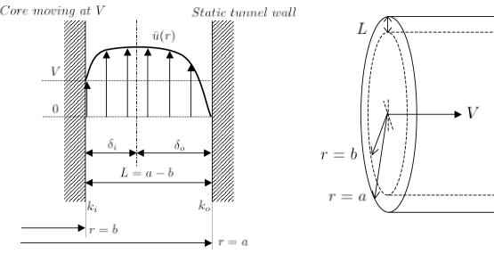
Figure 2: Geometry of the fully developed annulus velocity profile.

Here the boundary on the left represents the outer surface of the train at $r=b$, with surface roughness $k_{i}$ moving with velocity $V$. The boundary on the right represents the stationary tunnel wall surface at $r=a$ ($>b$) with surface roughness $k_{o}$. The flow adjacent to the train forms a boundary layer of thickness $\delta_{i}$. The no-slip boundary at the train surface is moving with velocity $V$ relative to the tunnel wall. The flow adjacent to the tunnel wall forms a boundary layer of thickness $\delta_{o}$ with the velocity equal to zero at the wall to satisfy the no-slip boundary condition. The distance between the surface of the train and the tunnel wall, $L=a-b$, is the sum of the two boundary layers, $\delta_{i}+\delta_{o}$. The flow profile, $u(r)$, is also shown in Figure 2. This profile is generated by the matching of two separate profiles for flow over the two boundary layers.

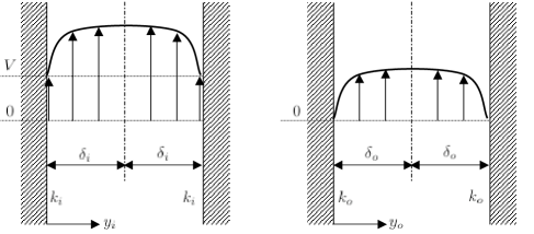
Figure 3: Two ducts containing the flow adjacent to the train (on the left) and the flow adjacent to the tunnel wall (on the right).

A method that can be used to arrive at the matched velocity profile is outlined in both Barrow and Pope (1987) and Shigechi et al. (1990). The process involves consideration of two ‘imaginary ducts,’ each twice the width of the two boundary layers $\delta_{i}$ and $\delta_{o}$ shown in Figure 2. These two ducts are shown in Figure 3.

The flow in each of the two ducts has the generic flow profile given by (1). The mean flow in the inner boundary layer adjacent to the train takes the form

$$u_{i}(y_{i})=v_{*i}\left(2.5\log\left(\frac{y_{i}}{k_{i}}\right)+8.5\right),$$ (6)

while the flow in the outer boundary layer adjacent to the tunnel wall takes the form

$$u_{o}(y_{o})=v_{*o}\left(2.5\log\left(\frac{y_{o}}{k_{o}}\right)+8.5\right).$$ (7)

There are four unknown parameters: the friction velocities, $v_{*i}$ and $v_{*o}$, and the boundary layer thicknesses, $\delta_{i}$ and $\delta_{o}$, associated with each of the two flow profiles. We now describe the four equations relating the parameters required for a solution.

Firstly, the sum of the two boundary layer thicknesses is equal to the gap between the train and tunnel wall such that

$$\delta_{i}+\delta_{o}=a-b.$$ (8)

Secondly, the mean velocity of the inner profile must match the mean velocity of the outer profile at the interface of the two boundary layers, $u_{i}(\delta_{i})+V=u_{o}(\delta_{o})$, giving

$$v_{*i}\left(2.5\log(1/k_{i})+8.5\right)+V=v_{*o}\left(2.5\log(1/k_{o})+8.5\right).$$ (9)

Thirdly, by continuity flux through the annulus must be equal to $Q$, the flow through the open tunnel as described earlier in this section. Integrating over the two boundary layers and allowing for the morion of the inner layer at velocity $V$ relative to the inner boundary layer implies that

$$Q=2\pi\int_{0}^{\delta_{i}}(b+y_{i})u_{i}(y_{i})dy_{i}+2\pi V\int_{0}^{\delta_{i}}y_{i}dy_{i}+2\pi\int_{0}^{\delta_{o}}(a-y_{o})u_{o}(y_{o})dy_{o}\,.$$ (10)

Substituting (6) and (7) into the above expression and evaluating the integral gives

$$Q=2\pi v_{*i}A_{i}+\pi(\delta_{i}^{2}+2b\delta_{i})+2\pi v_{*o}A_{o}\,,$$ (11)

where

$$A_{i}=\delta_{i}\left(6b+3.625\delta_{i}+\left(\left(2.5b+1.25\delta_{i}\right)\log(1/k_{i})\right)\right)$$ (12)

and

$$A_{o}=\delta_{o}\left(6a-3.625\delta_{o}+\left((2.5a-1.25\delta_{o})\log(1/k_{o})\right)\right).$$ (13)

The fourth and final relation is obtained by assuming that the flow profiles are fully developed so that there is no mean acceleration. Hence, the mean forces acting on the fluid must balance to zero. This requires $\tau/\delta=\text{constant}$, see Pope (2001, Section 7.1.2). It follows that

$$v_{*i}=v_{*o}\sqrt{\delta_{i}/\delta_{o}}\,.$$ (14)

The four relationships given by (8), (9), (11) and (14) can be used to solve for the previously noted unknowns numerically. This approach differs from that presented in Barrow and Pope (1987) and Shigechi et al. (1990): both rely on an assumed value of the annulus axial pressure gradient of the flow, which requires prior knowledge of the flow profile. The shear stress at the train surface and tunnel wall can be computed using (2) with $v_{*i}$ and $v_{*o}$ respectively.

The parameters for a typical tunnel section of the Piccadilly line are listed in Appendix A. Details of the computations required to generate the matched velocity profile are also given. The thickness $\delta_{i}$ of the inner boundary layer formed adjacent to the surface of the train is approximately $80$ millimeters. The boundary layer adjacent to the tunnel wall takes up the remaining $240$ millimeters. The shear stress at the tunnel wall for flow in the annulus, $\tau_{w}$ is approximately $3.2$ N/m². This is roughly one order of magnitude larger than the shear stress at the tunnel wall for the open tunnel flow given the same air flow rate.

2.4 Heat Transfer at the Tunnel Wall

The motivation behind the study of open tunnel and annulus flow profiles in the previous sections is to determine $\tau_{w}$, the shear stress at the tunnel wall. This is related to $h_{w}$, the coefficient of convective heat transfer between the tunnel air and wall, by the Reynolds analogy. The main results are briefly presented here. A full derivation is available in most heat transfer texts, including Grimson (1971) and Kreith and Bohn (1993). Detailed discussion of combined thermal and velocity boundary layers is given in Schlichting and Gersten (2000, Chapter 18).

The rate of heat transfer between the tunnel air into the tunnel wall is defined by Newton’s law of cooling such that

$$\dot{q}=h\left(f\left(t\right)-T\left(a,t\right)\right),$$ (15)

where $\dot{q}$ is the heat flux into the solid, $f(t)$ is the temperature of the air in the tunnel averaged over the tunnel cross-section, $h$ is the coefficient of convective heat transfer and $T(a,t)$ is the temperature of the wall surface $(r=a)$.

2.5 The Reynolds Analogy

The Reynolds analogy uses the fact that, when there is both a velocity and temperature boundary layer through a flow adjacent to a wall, there is a similarity between the momentum and energy equations for the flow and hence the velocity and temperature profiles. This similarity stems from the fact that heat transfer is proportional to the first derivative of temperature and shear stress is proportional to the first derivative of velocity over the boundary layer.

The Prandtl number of the fluid is defined as

$$Pr=\frac{C_{p}\mu}{K}=\frac{\nu}{\kappa}\,.$$ (16)

Here $C_{p}$ is the specific heat capacity, $K$ is the conductivity and $\kappa$ is the thermal diffusivity of the fluid. When $Pr$ is equal to $1$, the energy and momentum equations and therefore the temperature and velocity profiles are similar. In this case the Reynolds analogy hold exactly and the heat transfer coefficient can be computed as

$$h=\frac{\tau_{w}C_{p}}{\bar{u}}\,.$$ (17)

For air the Prandtl number, $Pr_{\mathrm{air}}=0.71$, so the Reynolds analogy is considered a reasonable approximation (Kreith and Bohn, 1993, p. 410). A number of empirical relations have been developed to provide more accurate approximations for specific geometries and Prandtl and Reynolds number ranges. These have not been considered in our paper.

Using the wall shear stress values computed for the Piccadilly Line tunnels in this section and appropriate constants for air, the heat transfer coefficients for open tunnel and annular flow can be computed using (17) as

• Open tunnel flow: $h=44$ W/m${}^{2}\cdot$K

• Annulus flow: $h=110$ W/m${}^{2}\cdot$K

Details of the parameters assumed and computations are given in Appendix A. Notice the large increase in the coefficient for the annular flow case, due to the high shear generated by passing trains.

3 Soil Temperature Response to an Impulse Change in Air Temperature

In this and the next section we consider the conduction of heat through the soil surrounding a tunnel of circular cross section with radius $a$. The temperature of the soil is governed by the one dimensional heat equation in radial coodinates,

$$\frac{\partial{T(r,t)}}{\partial{t}}=\kappa\left(\frac{\partial^{2}{T(r,t)}}{\partial{r^{2}}}+\frac{1}{r}\frac{\partial{T}}{\partial{r}}\right)\,.$$ (18)

Here $r$ is the radial coordinate, $t$ is time, $T(r,t)$ is the temperature of the solid in $a\leq r\leq\infty$ and $\kappa=K/\rho C$ is the thermal diffusivity of the solid, where $K$, $\rho$ and $C$ are the conductivity, density and specific heat capacity respectively.

A number of assumptions have been made in the above formulation of the one dimensional problem. Firstly, a single cross section of tunnel has been considered meaning that any heat conduction along the axis of the tunnel (perpendicular to the radial coordinate) is neglected. Secondly, it has been assumed that there is no angular dependence to the temperature profile; that there is not top or bottom to the tunnel. This infers that the tunnel wall is an infinite distance from any other heat source or boundary. The validity of these assumptions is discussed in more detail later later in this section. The geometry of the problem under consideration is shown in Figure 4.

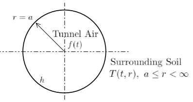
Figure 4: Tunnel of radius $r=a$, air temperature $f(t)$, heat transfer coefficient $h$.

Conductive heat transfer through the solid is driven by the difference between the air temperature within the tunnel, $f(t)$, and the surface temperature of the tunnel, $T(a,t)$. Convective heat transfer between the air and wall obeys Newton’s cooling law. Heat flux at the tunnel wall is continuous, which requires

$$-\frac{\partial{T(a,t)}}{\partial r}=H\left(f(t)-T(a,t)\right)~{},$$ (19)

where $H=h/K$, which is taken as a constant in this section (in Section 5 we investigate the effects of the short-term oscillations in $h$ due to passing trains). The boundary condition at infinity is

$$T(\infty,t)~{}\text{finite as}~{}r\rightarrow\infty\,.$$ (20)

For ease of computation we have taken $f(t)$ as the absolute temperature difference between the tunnel air and the ‘deep sink’ temperature of the soil. Hence $T(\infty,t)=0$, and $T(r,t)$ is the absolute temperature difference between the soil temperature within the thermal boundary layer around the tunnel and the constant ‘deep sink’ soil temperature.

Owing to the linearity of the problem, the temperature of the air in the tunnel, $f(t)$, can be expressed as the sum of any number of components. We have assumed that a sum of a generic steady and periodic component $f(t)=f_{s}+f_{p}(t)$. Physically the steady component is due to heat sources within the tunnel environment elevating the air temperature. The periodic components result from daily and seasonal fluctuations in ambient air temperature which make their way into the tunnel.

In this section we are investigate the behavior of temperature in the soil due to an instantaneous change in air temperature. The initial temperature of the soil is assumed constant, $T(r,0)=0$ for $a\leq r<\infty$—the tunnel wall and all of the surrounding soil are initially at the ‘deep sink’ temperature. The constant component of the air temperature is assumed to be $f_{s}=1$. Both of these assumptions can be made without loss of generality.

The long-term solution to this problem is the steady state $T(r)=f_{s}$ as $t\rightarrow\infty$. Here all the spatial and temporal derivatives eventually go to zero and hence the soil temperature approaches the air temperature. This steady state solution is sufficient where only the long-term behavior of the tunnel wall temperature is required. However, a solution of the transient behaviour is useful in that it gives the time needed to reach the steady state. This is of interest, for instance, in determining how long an underground rail system will operate before initial transients die out and peak temperatures are reached .

3.1 Solution of the Equation

Application of the Laplace transform to the governing equation (18) results in the subsidiary ordinary differential equation

$$\frac{d^{2}\bar{T}}{dr^{2}}+\frac{1}{r}\frac{d\bar{T}}{dr}-q^{2}\bar{T}=0\,,$$ (21)

where $p$ is the transform space, $\bar{T}$ is the transformation of $T$ and $q^{2}=p/\kappa$. This takes the form of the modified Bessel equation of order zero which has solution (Abramowitz and Stegun, 1965)

$$\bar{T}=BK_{0}(qr)\,,$$ (22)

where $B$ is a constants and the other linearly independent solution is ruled out by the condition at infinity (20). $B$ is determined from the Laplace transform of the boundary condition (19),

$$\bar{T}(r,t)=\frac{HK_{0}(qr)}{p\left(HK_{0}(qa)-qK_{1}(qa)\right)}\,.$$ (23)

Applying the inverse Laplace transform to (23),

$$T(r,t)=\frac{H}{2\pi i}\int_{\gamma-i\infty}^{\gamma+i\infty}\exp(\lambda t)\frac{K_{0}(\mu r)}{\lambda\left(HK_{0}(\mu a)-\mu K_{1}(\mu a)\right)}d\lambda\,,$$ (24)

where $\mu=\sqrt{\lambda/\kappa}$. The integral above contains a branch point at $\lambda=0$. The contour integral is taken over the usual “keyhole” contour.

We separate the real and imaginary components of the integral using the relationship

$$K_{0}\left(x\exp(i\pi/2)\right)=-\frac{1}{2}i\pi\left(J_{0}(x)-i\,Y_{0}(x)\right)\,,$$ (25)

and find

$$T(r,t)=\frac{2H}{\pi}\int_{0}^{\infty}\frac{du}{u}\,\exp(-\kappa u^{2}t)\\ \times\frac{J_{0}(ur)\left(uY_{1}(ua)+HY_{0}(ua)\right)-i\,Y_{0}(ur)\left(uJ_{1}(ua)+HJ_{0}(ua)\right)}{\left(uJ_{1}(ua)+HJ_{0}(ua)\right)^{2}+\left(uY_{1}(ua)+HY_{0}(ua)\right)^{2}}\,.$$ (26)

The solution presented above is adapted from the outline given in Carslaw and Jaeger (1959, §13.5).

Substituting appropriate parameters into (26) gives results for the Piccadilly Line tunnels. Here the tunnel radius, $a=1.7$ m, thermal conductivity of the soil is $K=0.35$ W/(m$\cdot$K) and the heat transfer coefficient $h=44$ and $h=110$ W/m${}^{2}\cdot$K for open tunnel and annulus flow respectively.

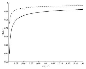
Figure 5: Tunnel wall surface temperature profiles for $h=44(-),110(-~{}-)$.

Figure 5 shows the behavior of the wall temperature against time for the two heat transfer coefficients for an impulse change in air temperature. Temperature at the wall surface approaches the air temperature faster for a larger value of $H$. The profiles for $h=44$ and $110$ reach 0.99 of the asymptotic value when $\kappa t/a^{2}=$ 0.2 and 0.02 respectively. This in turn corresponds to times of approximately 5 and 50 days respectively (see Appendix A for calculations).

4 Soil Temperature Response to Periodic Variations in Air Temperature

As discussed in Section 3, we write difference between the ground deep sink temperature and the air at any location in an underground tunnel as a steady and time-dependent component, $f(t)=f_{s}+f_{p}(t)$. The time varying component, due to diurnal and seasonal fluctuations in ambient temperature, is expected to be a periodic function of time. The response of the radial soil temperature profile $T(t,r)$ to the steady component was discussed in the previous section. In this section we deal with the fluctuating component.

A solution to the heat equation with $f_{p}(t)$ a periodic function of time can be found using the Laplace transform techniques used in the previous section. As was the case there, a decaying transient term will result from a branch point. There will also be two simple poles within the contour which can be evaluated using Cauchy’s Theorem. These simple poles give the limit cycle of the steady oscillating solution to the problem. The steady oscillating component of the solution is of greatest interest, as it describes the long-term behavior of temperature within the soil surrounding the tunnel, and hence heat flux through the walls.

In this section the limit cycle is found using assumptions about the form of the cycle rather than a Laplace transform. The Laplace transform is necessary to find the transient component of the solution associated with the oscillating solution, which is not considered here.

4.1 General Form of the Oscillating Solution

It is expected that the periodic components of the tunnel air temperature, $f_{p}(t)$, will produce periodic fluctuations of the same frequency in the temperature of the solid. Hence, the temperature field in the solid is expected to take the form

$$T(r,t)=e^{i\omega t}R(r)\,,$$ (27)

where $\omega$ is the frequency of fluctuation in $f_{p}(t)$ and $R(r)$ is independent of time. Substituting this form into (18) gives

$$r^{2}\frac{d^{2}R}{dr^{2}}+r\frac{dR}{dr}-\frac{i\omega}{\kappa}r^{2}R=0\,,$$ (28)

the modified Bessel’s equation of order zero. This has solution given by (22) with $q=\sqrt{{i\omega}/{\kappa}}$ and $B$ is a constant, and once again the boundary condition (20) has been applied. Substituting the solution (22) into the boundary condition at the tunnel wall (19) yields the constant $B$, hence

$$T(r,t)=\frac{Hf_{p}(t)K_{0}\left(\sqrt{\frac{i\omega}{\kappa}}r\right)}{HK_{0}\left(\sqrt{\frac{i\omega}{\kappa}}a\right)+\sqrt{\frac{i\omega}{\kappa}}K_{1}\left(\sqrt{\frac{i\omega}{\kappa}}a\right)}\,.$$ (29)

In order to extract the real component of the solution, the imaginary terms in the denominator and in the arguments of the modified Bessel functions must be separated. This is achieved by writing the modified Bessel function in terms of the real and imaginary components of the Kelvin function, $\mathrm{ker}_{\nu}$ and $\mathrm{kei}_{\nu}$ using the relation

$$e^{-\nu\pi i/2}K_{\nu}(xe^{\pi i/4})=\mathrm{ker}_{\nu}(x)+i\,\mathrm{kei}_{\nu}(x)\,.$$ (30)

The final relation can be greatly simplified when expressed in terms of the Kelvin function modulus, $N_{\nu}$, and phase, $\phi_{\nu}$, defined as

$$N_{\nu}(x)=\sqrt{\mathrm{ker}_{\nu}^{2}(x)+\mathrm{kei}_{\nu}^{2}(x)}\,,$$ (31)

$$\phi_{\nu}(x)=\arctan\left(\mathrm{kei}_{\nu}(x)/\mathrm{ker}_{\nu}(x)\right)\,.$$ (32)

The relations (30), (31) and (32) are given in Abramowitz and Stegun (1965).

Rewriting (29) in terms of the modulus and phase of Kelvin functions gives

$$T(r,t)=\frac{Hf_{p}(t)N_{0}(\omega^{\prime}r)\exp\left(i\phi_{0}(\omega^{\prime}r)\right)}{HN_{0}(\omega^{\prime}a)\exp\left(i\phi_{0}(\omega^{\prime}a)\right)+\sqrt{\frac{i\,\omega}{\kappa}}aN_{1}(\omega^{\prime}a)\exp\left(i\left(\phi_{1}(\omega^{\prime}a)+\frac{\pi}{2}\right)\right)}\,,$$ (33)

where $\omega^{\prime}=\sqrt{\omega/\kappa}$ is the inverse length scale to which the oscillating temperature variations penetrate the solid.

Specifying the form of the periodic air temperature variations to be $f_{p}(t)=\sin(\omega t+\epsilon)$, which is still of a general enough form to accommodate the desired fluctuations, helps to simplify the expression further.

Using Euler’s formula and the harmonic addition theorem, the denominator of (33) can be separated into real and imaginary parts ($\alpha+i\,\beta$). Multiplying numerator and denominator by the complex conjugate of this gives

$$T(r,t)=\frac{HN_{0}(\omega^{\prime}r)\sin\left(\omega t+\epsilon+\phi_{0}(\omega^{\prime}r)-\arctan(\beta/\alpha)\right)}{\sqrt{\alpha^{2}+\beta^{2}}}\,,$$ (34)

where

$$\alpha=HN_{0}(\omega^{\prime}a)\cos\left(\phi_{0}(\omega^{\prime}a)\right)\\ +\frac{\omega^{\prime}}{\sqrt{2}}N_{1}(\omega^{\prime}a)\left(\cos\left(\phi_{1}(\omega^{\prime}a)+\pi/2\right)-\sin\left(\phi_{1}(\omega^{\prime}a)+\pi/2\right)\right),$$ (35)

$$\beta=HN_{0}(\omega^{\prime}a)\sin(\phi_{0}(\omega^{\prime}a))\\ +\frac{\omega^{\prime}}{\sqrt{2}}N_{1}(\omega^{\prime}a)\left(\cos\left(\phi_{1}(\omega^{\prime}a)+\pi/2\right)+\sin\left(\phi_{1}(\omega^{\prime}a)+\pi/2\right)\right).$$ (36)

The fact that the analytic solution to the problem (34) is stated in terms of the modulus and phase of Kelvin functions means that its behaviour may not be immediately apparent. The graphs below illustrate its general features. In all the computations we used unity for all parameters other than $\omega$, which was set to $2\pi$, so that $f_{p}(t)$ has period one and $\epsilon$, which was set to zero. The Kelvin functions have been computed using asymptotic approximations and code given in Jin and Zhang (1996).

Figure 6 shows the air, $f_{p}(t)=\sin(2\pi t)$, and tunnel surface temperature, $T(a,t)$, plotted against time for one period of oscillation. The temperature at the wall surface has the same period as the air temperature, but has a smaller amplitude and is out of phase with (slightly lagging) the wall temperature.

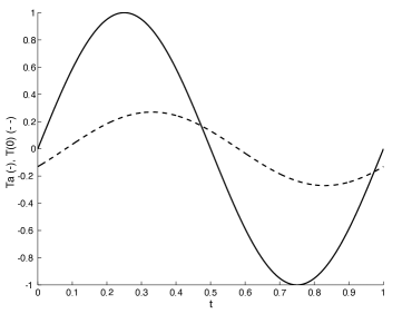
Figure 6: Air (–) and tunnel wall (- -) temperatures vs time.

Figure 7 is a plot of temperature against time at the tunnel surface and at progressive depths into the solid. This plot also shows that there is a decay in magnitude of the temperature oscillations as we move into the solid and a continual shift in the phase of the temperature oscillations.

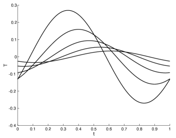
Figure 7: Temporal variation of temperature various depths: $r=a$, and $a+0.25,0.5,0.75,1,1.5,2$.

The general form of the solution (34) has three distinct components relating to the amplitude of the tunnel wall temperature, the decay of the temperature with radial distance from the tunnel wall and the phase of temperature oscillations through a soil thermal boundary layer when compared to the air temperature oscillations.

The amplitude component of the solution, including the radial component of the solution evaluated at the tunnel wall is

$$\frac{HN_{0}(\omega^{\prime}a)}{\sqrt{\alpha^{2}+\beta^{2}}}\,,$$ (37)

where $\alpha$ and $\beta$ are given by (35) and (36) respectively. Although this term is a constant for any given problem, it will vary with the value of the parameters: $a,H=h/K$ and $\omega^{\prime}=\sqrt{\omega/\kappa}$.

The amplitude component (37) plotted against the parameter $h/K$ is shown in Figure 8 for typical values for the Piccadilly line tunnels (see Appendix A). The two profiles plotted are for oscillations with periods of one day and one year. As $h/K$ increases, the constant term asymptotically approaches unity. That is, the temperature at the wall surface $r=a$ approaches the oscillating air temperature. If the convective heat transfer coefficient, $h$, is very large or if the thermal conductivity of the solid, $K$, is very small, then the oscillations in the air temperature are also seen in the wall temperature. Further, this approach for increasing $h/K$ is dependent on the frequency of oscillation, $\omega$. For the same value of $h/K$, the wall surface temperature approaches the air temperature more quickly for lower frequency oscillations. This is shown in Figure (8), as the approach for yearly oscillations is more pronounced than for daily oscillations.

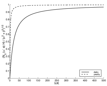
Figure 8: Amplitude component (37).

The radial component of the periodic solution is $N_{0}(\omega^{\prime}r)$. This reduces the magnitude of any temperature variation with distance from the tunnel wall in proportion to $\sqrt{\omega^{\prime}}$ defining the depth of a thermal boundary layer around the tunnel which is affected by oscillating air temperatures within the tunnel. This is shown in Figure 9, a plot of $N_{0}(\sqrt{\omega/\kappa}r)$ against time normalised to $N_{0}(\sqrt{\omega/\kappa}a)$.

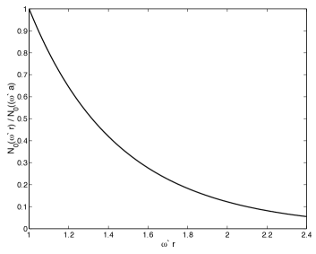
Figure 9: Kelvin modulus $N_{0}(\sqrt{\omega/\kappa}r)$, showing the decay of temperature with distance from wall.

The magnitude of the temperature fluctuations has reduced to approximately 0.1 that of the fluctuations at the wall surface when $\omega`r=2.2$. Using parameters for the Piccadilly line tunnels, diurnal temperature fluctuations die out to 0.1 of the peak value at the tunnel wall in approximately 0.1 meters. Yearly fluctuations die out within approximately 1.8 meters of the tunnel wall (see Appendix A for calculations). For the analogous problem in Cartesian coordinates, this decay with distance from a boundary is exponential, $\exp(-\omega x/\sqrt{2})$ (Carslaw and Jaeger, 1959, §2.6).

The periodic component of the solution for an air temperature of $\sin(\omega t+\epsilon)$ is

$$\sin\left(\ t+\epsilon+\phi_{0}(\omega^{\prime}r)-\arctan(\beta/\alpha)\right)\,.$$ (38)

The two additional arguments of the periodic function change the phase of the temperature oscillations in the solid. In general, the oscillations at the tunnel wall will be out of phase with the oscillations in air temperature. The phase difference will also change with distance from the wall by the component $\phi_{0}(\omega^{\prime}r)$. This effect is shown in Figure (7). As we move further into the solid the temperature oscillations not only reduce in amplitude, but also experience a continual phase lag, also a function of the oscillating frequency. This effect has been measured in the soil surrounding London Underground tunnels—a plot of yearly oscillations in soil temperature at increasing distance from a tunnel wall is given in Ampofo et al. (2004, Fig. 2).

4.2 Heat Flux through the Tunnel Wall

We have presented the main results of this section in terms of the oscillating temperature fields that form a thermal boundary layer around the tunnel. Computationally, however, these results are more useful when expressed in terms of the heat flux through the tunnel wall, $\dot{q}(r,t)$, defined as

$$\dot{q}(r,t)=-K\frac{\partial T(r,t)}{\partial r}\,$$ (39)

where we take the spatial derivative of the Bessel form of the solution, (29), containing both real and imaginary parts as both will contribute to the real part of the flux term. This yields

$$\dot{q}(r,t)=\frac{hf_{p}(t)N_{1}(\omega^{\prime}a)}{\sqrt{\alpha^{2}+\beta^{2}}}\biggl{[}\cos\left(\phi_{1}(\omega^{\prime}a)+\pi/2+\arctan\left(\frac{\alpha-\beta}{\alpha+\beta}\right)\right)\\ +i\,\left(\cos(\phi_{1}(\omega^{\prime}a)+\pi/2-\arctan\left(\frac{\alpha+\beta}{\alpha-\beta}\right)\right)\biggr{]}\,.$$ (40)

We write the right-hand side of (40) as $\dot{q}_{\mathrm{r}}+i\,\dot{q}_{\mathrm{i}}$. Both the real and imaginary parts are used in calculations in Section 5, where the coupled relationship between tunnel air and surface temperatures is investigated. The real component $\dot{q}_{\mathrm{r}}$ is only required for the explicit form of the flux as given below. For the case where $f_{p}(t)=\sin(\omega t+\epsilon)$, the final relationship becomes

$$\dot{q}(a,t)=\frac{hN_{1}(\omega^{\prime}a)}{\sqrt{\alpha^{2}+\beta^{2}}}\,\cos\left(\omega t+\epsilon+\phi_{1}(\omega^{\prime}a)+\arctan\left(\frac{\alpha-\beta}{\alpha+\beta}\right)\right)\,.$$ (41)

With this we have arrived at an explicit relationship for the heat flux into the soil surrounding a cross section of tunnel due to periodic oscillations in the tunnel air temperature. In practice this quantifies the cooling effect that the thermal mass of the soil can provide by rejecting heat during the night or the winter and absorbing it during the day or the summer. In the next Section we investigate the effect of the rapidly varying heat transfer coefficient due to passing trains on this result, which assumed $h$ is a constant.

5 Soil Temperature Response to Rapidly Fluctuating Heat Transfer Coefficient

In this section we consider the effects of varying heat transfer coefficient $h$ as described in Section 2. These fluctuations are caused by train movements and are treated as events that occur over a time period of several minutes, the effects of which have been ignored in the previous two sections.

Throughout this and subsequent sections an averaging function, denoted by $\langle\cdot\rangle$, over the short time period $\varepsilon$ is defined as

$$\langle\cdot\rangle=\frac{1}{\varepsilon}\int_{0}^{\varepsilon}\cdot~{}dt\,.$$ (42)

This section is divided into three parts. In Section 5.1 we examine the standard assumptions that temperature in a tunnel does not fluctuate over short time scales. In Section 5.2 we drop this assumption and show that the long-time heat flux is modified by short-term correlations between the heat transfer coefficient and the change of temperature in the tunnel.

5.1 Fluctuations Independent of Air Temperature

A first approximation of the effect of a rapidly fluctuating heat transfer coefficient can be made by assuming that temperature fluctuations occur independently of any changes in tunnel air temperature and on a much shorter time scale. It is typically assumed that all fluctuations in tunnel air temperature have a period of either one day or one year and are due to diurnal and seasonal fluctuations in external air temperature drawn into the tunnels by the train piston effect. Assuming a typical train headway (time between subsequent trains) of two minutes ($\varepsilon=120$ seconds), the periods of daily and yearly oscillations expected in the tunnel air ($f_{\varepsilon}(t)$) and surrounding soil ($T(r,t)$) are larger by factors of approximately $10^{4}$ and $10^{7}$.

As any changes in air and soil temperature occur over a period much longer than $\varepsilon$, the averaging operator (42) has no effect, that is $\langle f_{\varepsilon}(t)\rangle=f_{\varepsilon}(t)$ and $\langle T(r,t)\rangle=T(r,t)$, and the governing heat equation (18) is invariant under averaging. Averaging the boundary condition (19) gives the relationship

$$-\frac{\partial T(a,t)}{\partial r}=\langle H(t)\rangle\bigl{(}f_{\varepsilon}(t)-T(a,t)\bigr{)}.$$ (43)

Under these assumptions the heat transfer coefficient can simply be time averaged over a whole number of oscillations and treated as a constant. It follows that the results presented in the previous sections hold for a time averaged heat transfer coefficient $\langle h(t)\rangle$. This approach is generally used engineering calculations such as Barrow and Pope (1987).

5.2 Including Short-Term Fluctuations in Air Temperature

The assumptions detailed above are, however, flawed. As a train approaches a station and brakes, the kinetic energy possessed by the train and passengers is converted to heat energy. Train-generated heat accounts for as much as eighty five percent of the heat load within a typical London Underground station (Abi-Zadeh et al., 2003). It is therefore reasonable to assume that temperatures within underground rail tunnels will fluctuate, to some extent, over the same short time scales at which the heat transfer varies as both are caused by the passing of a train.

A better assumption is therefore that the tunnel air temperature does vary over the time scale $\varepsilon$, so $\langle f_{\varepsilon}(t)\rangle\neq f_{\varepsilon}(t)$. However, the large thermal inertia associated with the tunnel walls means that the wall surface temperature $T(a,t)$ will not be affected on this short time scale. This can be shown using the previous analytic solution (34) for an oscillating air temperature with $\omega=\varepsilon=2\pi/120$ radians per second.

Under the above assumptions the boundary condition (19) becomes

$$-\frac{\partial T(a,t)}{\partial r}=\langle H(t)f_{\varepsilon}(t)\rangle-\langle H(t)\rangle T(a,t)\,.$$ (44)

Hence, the solution to the heat equation given as (40) becomes

$$\langle\dot{q}(a,t)\rangle=\frac{K\langle H(t)f_{\varepsilon}(t)\rangle N_{1}(\omega^{\prime}a)}{\sqrt{\alpha^{2}+\beta^{2}}}\,\cos\left(\phi_{1}(\omega^{\prime}a)+\arctan\left(\frac{\alpha-\beta}{\alpha+\beta}\right)\right)$$ (45)

for the short-term average where $\alpha$ and $\beta$ now contain $\langle H\rangle$ rather than $H$. Note that if the short-term fluctuations in $f_{\varepsilon}(t)$ are ignored the heat flux (45) vanishes. If $H(t)$ and $f_{\varepsilon}(t)$ are statistically independent of each other, then $\langle H(t)f_{\varepsilon}(t)\rangle=\langle H(t)\rangle\langle f_{\varepsilon}(t)\rangle$, and the short-term average of each function is all that is required. However, this is not the case as the short-term fluctuations in both $H(t)$ and $f_{\varepsilon}(t)$ are both caused by the passage of trains through a tunnel.

As discussed in Section 4, the heat transfer coefficient $H(t)$ can be assumed to take a base value of $H_{1}$ when there is a train passing a particular point in a tunnel, and a lower value of $H_{2}$ when a train is not present. Although the air flows before and after the passage of the train are likely to be complicated, $H(t)$ can be approximated by a step function. Normalising the short-term fluctuations ($\varepsilon=1$), and defining the fraction of the train service headway for which a train is passing any given point in a tunnel as $\sigma$, which can be computed from the train headway, average speed and length (see Appendix A for assumed values and computations), then

$$H(t)=\begin{cases}H_{1}\,,\quad&\text{for }0<t<\sigma\,;\\ H_{2}\,,&\text{for }\sigma<t<1\,.\end{cases}$$ (46)

The short-term behavior of the air temperature in a tunnel as a train passes is somewhat more difficult to predict. Detailed output from a numerical simulation can be used or measurements made in an existing tunnel to confirm any assumptions or simulations. For ease of computation, however, we have not unrealistically assumed that these fluctuations in air temperature are sinusoidal with a generic phase lead or lag, $\varphi$, to show the effects of $H(t)$ and $f_{\varepsilon}(t)$ being in or out of phase with each other:

$$f_{\varepsilon}(t)=\sin(2\pi t/\varepsilon+\varphi).$$ (47)

A more complicated form of $f_{\varepsilon}(t)$ can be represented by a Fourier series. All subsequent calculations would then be essentially the same as those presented here. The averaged forcing term is

$$\langle H(t)f_{\varepsilon}(t)\rangle=H_{1}\int_{0}^{\sigma}\sin(2\pi t+\varphi)dt+H_{2}\int_{\sigma}^{1}\sin(2\pi t+\varphi)dt\,.$$ (48)

Hence

$$\langle H(t)f_{\varepsilon}(t)\rangle=\frac{1}{\pi}(H_{1}-H_{2})\sin(\pi\sigma)\sin(\pi\sigma+\varphi)\,.$$ (49)

Calculations have been carried out using the values for $H_{1}$, $H_{2}$, $\sigma$, and $\varepsilon$ from the Piccadilly line parameters given in Appendix A. A short-term temperature oscillation with a magnitude of one degree centigrade has been assumed. This is an estimate, and detailed measurements or simulations are required for any particular application.

The averaged forcing term is a sinusoidal function of the phase difference between $H(t)$ and $f_{\varepsilon}(t)$. For the parameters above the amplitude is approximately 18.5 for a relatively small fluctuation in air temperature. Physically, this means that heat transfer into the wall is increased if the air temperature is warmer when a train is present and the heat transfer coefficient is greater. As the train is a heat source, we expect this to be the case. Hence, ignoring the correlation between short-term oscillations in air temperature and heat transfer coefficient will underestimate heat transfer to the wall.

6 Heat Transfer from a Tunnel of Finite Length

Analytic solutions presented thus far have concentrated on a single location in a tunnel. In all circumstances a generic air temperature, $f(t)$, has been considered. However, in an underground environment the temperature of the air and surrounding soil are coupled. If there is heat flux from the air into the tunnel wall the air temperature is cooled.

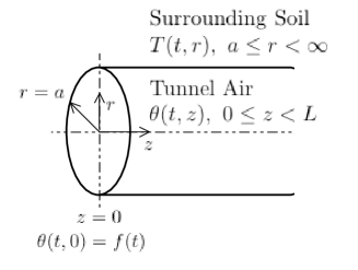
Figure 10: Tunnel of radius $r=a$ and length $z=L$, air temperature $\theta(t,z)$.

In this section air temperature within a tunnel, $\theta(t,z)$, is assumed to be a function of both time and the axial distance along the tunnel $z$. It is assumed that the temperature at the beginning of the tunnel is known and is a simple harmonic function of time,

$$\theta(t,0)=f(t)=D\exp(i\omega t).$$ (50)

A version of the solution presented here is given in Peavy (1961), where the homogeneous problem is considered. This does not allow for the heat flux due to short-term fluctuations, or any other inhomogeneous heat generation within the tunnel, so is of limited use.

The equation governing the temperature of air flowing axially through a tunnel, $\theta(t,z)$, where $z$ is the axial coordinate is

$$MC_{p}\left(\frac{\partial\theta(t,z)}{\partial t}+u\frac{\partial\theta(t,z)}{\partial z}\right)+\dot{q}+h\left(\theta(t,z)-T(t,a)\right)=0\,.$$ (51)

Here $M=\rho_{a}a/2$ is the mass of air per unit area of tunnel wall and $C_{p}$ is the specific heat of air in the tunnel, assumed to be a constant for the temperature ranges under consideration.

The first term represents the change in air temperature with time due to the thermal mass of the air in the tunnel, heat flux through the tunnel by convection at an average velocity $u$. The second term accounts for a general heat flux $\dot{q}$. This term accounts for the additional flux due to the short-term fluctuations in air temperature and heat transfer coefficient. Any other continuous heat sources along the length of the tunnel can also be accounted for here. The third term accounts for heat flux through the tunnel wall due to the temperature difference between the tunnel air, $\theta(t,z)$ and the wall surface temperature along the tunnel, $T(a,t;z)$. This heat flux is assumed to be purely radial (i.e., no heat flux through the surrounding soil along the tunnel $z$ axis). As a result, this term can be expressed as the Bessel formulation of the heat conduction given previously. Hence the tunnel wall flux can be considered as a complex term multiplied by the tunnel air temperature $(\dot{q}_{\mathrm{r}}+i\,\dot{q}_{\mathrm{i}})\theta(t,z)$, where $\dot{q}_{\mathrm{r}}$ and $\dot{q}_{\mathrm{i}}$ are given by (40) and the driving air temperature term $\theta(t,z)$ is now a function of the axial distance down the tunnel, so replaces $f(t)$.

With the above assumptions, the tunnel air temperature can be separated into a function of the tunnel axis and a time oscillating component as

$$\theta(t,z)=\exp(i\omega t)Z(z)\,.$$ (52)

The solution to Eq. (51) is then

$$\theta(t,z)=\frac{b}{a}\left(1-\exp(-az)\right)+D\exp(i\omega t-az),$$ (53)

where

$$a=\frac{1}{u}\left(\frac{A}{MC_{p}}+i\,\left(\omega+\frac{B}{MC_{p}}\right)\right),\qquad b=\frac{\dot{q}}{MC_{p}u}\,,$$ (54)

and we applied boundary condition (50) at $z=0$.

Extracting the real part of (53) gives the explicit solution for air temperature within the tunnel as a function of time and axial distance,

$$\theta(t,z)=\frac{\dot{q}}{MC_{p}(E^{2}+F^{2})}\\ \times\left[E-E\exp\left(-\frac{zE}{u}\right)\cos\left(\frac{zF}{V}\right)+F\exp\left(-\frac{zE}{V}\right)\sin\left(\frac{zF}{V}\right)\right]\\ +D\exp\left(-\frac{zE}{V}\right)\cos\left(\omega t-\frac{zF}{V}\right)$$ (55)

where

$$E=\frac{A}{MC_{p}}\,,\qquad F=\omega+\frac{B}{MC_{p}}\,.$$ (56)

The solution given by (55) has two distinct components. The first comes from the inhomogenous term in the governing equation and hence is proportional to $\dot{q}$. This gives the effect of a continual heat source or sink along the tunnel which is independent of either the air or tunnel wall temperature. Such loads can include heat from lighting or other equipment along the tunnel or the additional heat flux due to the correlation between short-term fluctuations in air temperature and heat transfer coefficient, as given in Section 5.2. The second component shows that fluctuations in the inlet air temperature decay exponentially along the tunnel axis as $\exp(-{zA}/{MC_{p}u})$.

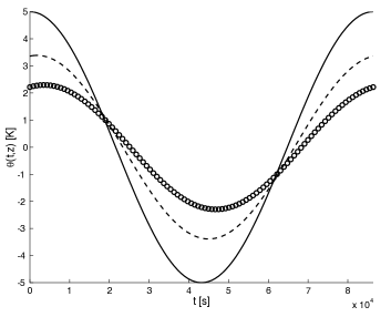
Figure 11: Daily temperature fluctuations at the beginning (–), middle (- -) and end (o) of a tunnel.

Figure 11 shows inlet air temperature fluctuations of amplitude 5 degrees Celsius at the beginning, middle and end of a 1000 m long tunnel for daily temperature variations. The temperature fluctuations are damped as they propagate along the tunnel. There is also a phase shift in the fluctuations along the tunnel.

For the parameters involved in this particular application the lower frequency yearly oscillations are almost unaffected by the thermal mass of the soil. This means that, once the initial transients die away, seasonal oscillations in ambient air temperature do not affect the peak air temperature in the tunnel. The majority of the damping is due to daily oscillations. This was suggested by the results presented in Section 4 (see Figure 5 where the tunnel surface temperature closely approached the air temperature and hence greatly reduced heat flux over the wall).

Figure 12 shows the decay of the peak daily temperature along the length of the tunnel. By the end of the tunnel (1000 m) the amplitude of the fluctuations is approximately half this value.

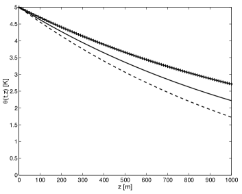
Figure 12: Decay of peak daily temperature along a tunnel with varying tunnel heat load.

The effect of the inhomogeneous term $\dot{q}$ is also shown in Figure 12. The three different profiles are for $\dot{q}=$ 0, -10 (- -) and +10 (+) W/m²/m (Watts per square meter of tunnel surface per meter of tunnel length). Depending on the sign of the flux term, the air temperature along the tunnel is shifted either up or down, as expected.

7 Summary

This paper has presented analytic solutions to a number of air flow, heat convection and heat condition problems. These include the following:

• A model of the turbulent air flow profile through both an open circular tunnel and in the annulus between a stationary circular tunnel with a moving concentric core. This is used to estimate the air flow profile and hence the convective heat transfer coefficient for an open tunnel and between the tunnel wall and a moving train.

• The evolution of the temperature of the soil surround an underground tunnel in response to an instantaneous change in air temperature within the tunnel. This is used to estimate the period of time it takes for the soil around a new tunnel to reach a steady operating temperature.

• The limit cycle thermal response of the soil surrounding a tunnel to an oscillating air temperature within the tunnel. This is used to quantify the effect of the thermal mass of the soil on temperatures within the tunnel.

• The effect of a correlation between short-term fluctuations in air temperature and heat transfer coefficient, both the result of passing trains, is to increase the mean soil temperature.

• Finally, a model is derived that accounts for the propagation of temperature fluctuations along the axis a tunnel of finite length and through the surrounding soil (perpendicular to the tunnel axis).

The analytical model for the coupled evolution of air temperature within and soil temperature around an underground rail tunnel can be applied to a simple rail tunnel as described, or to other engineering applications where the effect of periodic temperature variations influence an effectively infinite solid. These include modelling the heat dissipation from a cable tunnel (used for underground high voltage power distribution) and the response of the soil temperature to ground coupled heat pumps. The more detailed treatment of the thermal mass surrounding a tunnel would allow existing models, such as that developed by Ampofo et al. (2004), to quantify the effects potential benefits of flushing the London Underground with cool night air, for example.

Further work on this subject could be undertaken to apply the underlying analytical approach to more complicated boundary conditions. While some tunnels are lined with concrete, which is thermally similar to the surrounding soil, many tunnels are lined with cast iron segments, which are not. An obvious progression of the work presented in this paper is to make an allowance for tunnel linings. Further, tunnels are often within the thermal boundary layers of adjacent tunnels or the ground surface. As a result the assumption that the tunnel is surrounded by an infinite amount of soil with no additional heat loads is not valid.

Appendix A Physical Parameters

Table 1: Physical constants from Kreith and Bohn (1993)

Density (air)	$\rho_{a}$	1.16	kg/m3
Absolute Viscosity (air)	$\mu$	1.82$\times 10^{-5}$	N.s/m2
Dynamic Viscosity (air)	$\nu$	1.57$\times 10^{-5}$	m2/s	$\nu=\mu/\rho_{a}$
Thermal Conductivity (air)	Ka	2.51$\times 10^{-2}$	W/m.K
Specific Heat (air)	Cpa	1012	J/kg.K
Density (soil)	$\rho_{s}$	1500	kg/m3
Specific Heat (soil)	Cps	1842	J/kg.K
Theramal Conductivity (soil)	Ks	0.35	W/m.K
Thermal Diffusivity (soil)	$\kappa$	1.27 $\times 10^{-7}$	m2/s

Table 2: Piccadilly Line Parameters from Abi-Zadeh et al. (2003)

Tunnel Radius	$a$	1.70	m
Tunnel CSA	$A_{t}$	9.07	m2	$At=\pi a^{2}$
Train CSA	$A_{v}$	6.00	m2
Train Radius (equivalent)	$b$	1.38	m	$b=(A_{v}/\pi)^{1/2}$
Annulus Area	$A_{a}$	3.07	m2	$A_{a}=A_{t}-A_{v}$
Wall Roughness	$k_{o}$	0.01	m	typical
Train Surface Roughness	$k_{i}$	0.01	m	typical
Train Speed	$V$	14.0	m/s	typical
Average Tunnel Air Velocity	$U_{t}$	10.0	m/s	assumed
Tunnel Air Flux	$Q$	90.7	m3/s	$Q=U_{t}\times A_{t}$
Average Annulus Air Velocity	$U_{a}$	29.5	m/s	$U_{a}=Q/A_{a}$
Train Headway	$hwy$	120	s	time between trains
Train Length	$L$	183	m
Train Passing Time	$t_{pass}$	13.1	s	$t_{pass}=L/V$
Prop. of time Train Present	$\sigma$	0.11	-	$\sigma=t_{pass}/hwy$
Angular Freq. (short-term)	$\omega_{\varepsilon}$	5.23 $\times 10^{-2}$	rad/s	$\omega_{\varepsilon}=2\pi/hwy$

Table 3: Open Tunnel Flow

Reynolds Number	$Re$	1.08 $\times 10^{6}$	-	$Re=U_{t}a/\nu$
Friction Velocity	$v_{*}$	0.615	m/s	$v_{*}=Q/(2\pi a^{2}(2.375+1.25\log(1/k_{o}))$
Flow Type	$F_{t}$	392	-	$F_{t}=v_{*}k_{o}/\nu$
Wall Shear Stress	$\tau_{w}$	0.439	N/m2	$\tau_{w}=\rho_{a}v_{*}^{2}$
Tunnel Heat Transfer Coeff.	$h_{t}$	44.4	W/m2.K	$h_{t}=\tau_{w}C_{pa}/U_{t}$

Table 4: Train / Tunnel Annulus Flow

Reynolds Number	$Re$	1.20 $\times 10^{6}$	-	$Re=2U_{a}(a-b)/\nu$
Inner flow integral	$A_{i}$	2.00	-	$A_{i}=d_{i}(6b+3.625d_{i}+(2.5b+1.25d_{i})(\log(1/k_{i})))$
Outer flow integral	$A_{o}$	6.60	-	$A_{o}=d_{o}(6a+3.625d_{o}+(2.5a-1.25d_{o})(\log(1/k_{o})))$
Inner Friction Velocity	$v_{*i}$	0.958	m/s	$v_{*i}=v_{*o}(d_{i}/d_{o})^{1/2}$
Inner Boundary Layer	$d_{i}$	8.01 $\times 10^{-2}$	m	Solved Numerically
Outer Friction Velocity	$v_{*o}$	1.66	m/s	$v_{*o}=(Q-2\pi v_{*i}A_{i}-\pi Vv_{*i}(d_{i}^{2}+2bd_{i}))/(2\pi A_{o})$
Outer Boundary Layer	$d_{o}$	0.24	m	$d_{o}=a-b-d_{i}$
Flow Type (wall)	$F_{tw}$	1057	-	$F_{tw}=v_{*o}k_{o}/\nu$
Flow Type (train)	$F_{tt}$	611	-	$F_{tt}=v_{*i}k_{i}/\nu$
Wall Shear Stress	$\tau_{w}$	3.19	N/m2	$\tau_{w}=\rho_{a}v_{*o}^{2}$
Train Shear Stress	$\tau_{t}$	1.06	N/m2	$\tau_{t}=\rho_{a}v_{*i}^{2}$
Annulus Heat Transfer Coeff.	$h_{v}$	110	W/m2.K	$h_{w}=\tau_{w}C_{pa}/U_{a}$

Table 5: Effective Heat Transfer Coefficient

Open Tunnel Coefficient	$H_{t}$	127	m-1	$H_{t}=h_{t}/K_{s}$
Non-dim decay time	$t_{d}$	0.20	-	$t_{d}=\kappa t/a^{2}$
Decay Time (open tunnel)	$t$	4.56 $\times 10^{6}$	s	$t=t_{d}a^{2}/\kappa$
Annulus Coefficient	$H_{v}$	314	m-1	$H_{v}=h_{v}/K_{s}$
Non-dim decay time	$t_{d}$	0.02	-	$t_{d}=\kappa t/a^{2}$
Decay Time (annulus)	$t$	4.56 $\times 10^{5}$	s	$t=t_{d}a^{2}/\kappa$

Table 6: Decay of Temperature Fluctuations with Radial Distance

Non-dim. decay distance	$d_{d}$	2.2	-	from Figure 3.5
Period (yearly oscillations)	$p_{y}$	3.15 $\times 10^{7}$	s
Angular Freq. (yearly)	$\omega_{y}$	1.99 $\times 10^{-7}$	rad/s	$\omega_{y}=2\pi/p_{y}$
Therm. bndry layer (yearly)	$L_{y}$	1.8	m	$L_{y}=d_{d}/(\omega_{y}/\kappa)^{1/2}$
Period (daily oscillations)	$p_{d}$	8.64 $\times 10^{4}$	s
Angular Freq. (daily)	$\omega_{d}$	7.27 $\times 10^{-5}$	rad/s	$\omega_{d}=2\pi/p_{d}$
Therm. bndry layer (daily)	$L_{d}$	0.1	m	$L_{d}=d_{d}/(\omega_{d}/\kappa)^{1/2}$

References

- Abi-Zadeh et al. (2003) Abi-Zadeh, D., Casey, N., Sadokierski, S., Tabarra, M. (2003) “King’s Cross St Pancras Underground Station Redevelopment: Assessing the Effects on Environmental Conditions,” Underground Construction 2003 Conference Proceedings, pp. 641–653.
- Abramowitz and Stegun (1965) Abramowitz, M., Stegun I. A. (1964) “Handbook of Mathematical Functions,” Dover.
- Ampofo et al. (2004) Ampofo, F., Maidment, J., Missenden, J., (2004) ”Underground Railway Environment in the UK Part 2: Investigation of Heat Load,” Applied Thermal Engineering 24, pp. 633–645, 2004
- Barrow and Pope (1987) Barrow, H., Pope, C. W. (1987) “A Simple Analysis of Flow and Heat Transfer in Railway Tunnels,” International Journal of Heat and Fluid Flow, Vol 8, No 2, pp. 119–123, 1987.
- Carslaw and Jaeger (1959) Carslaw, H. S., Jaeger, J. C. (1959) “Conduction of Heat in Solids,” 2nd Edition, Clarendon Press.
- Grimson (1971) Grimson, J. (1971) “Advanced Fluid Dynamics and Heat Transfer,” McGraw-Hill.
- Huang and Chun (2003) Huang, S., Chun, C. H. (2003) “A Numerical Study of Turbulent Flow and Conjugate Heat Transfer in Concentric Annuli with Moving Inner Rod,” International Journal of Heat and Fluid Flow, Vol. 46, pp. 3707–3716 (2003).
- Jin and Zhang (1996) Jin, J., Zhang, S.-J. (1996) “Computation of Special Functions,” Wiley
- Kreith and Bohn (1993) Kreith, F., Bohn, M. S. (1993) “Principles of Heat Transfer,” 5th Edition, West Publishing Company.
- Patankar and Spalding (1970) Patankar, S. V., Spalding, D. B. (1970) “Heat and Mass Transfer in Boundary Layers,” 2nd Edition, Intertext Publishing.
- Peavy (1961) Peavy, B. A. (1961) “Heating and Cooling of Air Flowing Through an Underground Tunnel,” Journal of Research of National Bureau of Standards, Vol. 67C, No. 3.
- Pope (2001) Pope, S. B. (2001) “Turbulent Flows,” Cambridge University Press.
- Schlichting and Gersten (2000) Schlichting, H., Gersten, K. (2000) “Boundary Layer Theory,” 8th Edition, Springer-Verlag.
- Shigechi et al. (1990) Shigechi, T., Kawae, N., Lee, Y. (1990) “Turbulent Fluid Flow and Heat Transfer in Concentric Annuli with Moving Cores,” International Journal of Heat and Fluid Flow, Vol 33, No 9, pp. 2029–2037, 1990.