Isolated Eigenvalues of the Ferromagnetic Spin-$J$ XXZ Chain with Kink Boundary Conditions
Jaideep Mulherkar^a, Bruno Nachtergaele^a, Robert Sims^a, Shannon Starr^b

^aDepartment of Mathematics, University of California, Davis, Davis, CA 95616-8633, USA
^bDepartment of Mathematics, University of Rochester, Rochester, NY 14627, USA

Abstract:

We investigate the low-lying excited states of the spin $J$ ferromagnetic XXZ chain with Ising anisotropy $\Delta$ and kink boundary conditions. Since the third component of the total magnetization, $M$, is conserved, it is meaningful to study the spectrum for each fixed value of $M$. We prove that for $J\geq 3/2$ the lowest excited eigenvalues are separated by a gap from the rest of the spectrum, uniformly in the length of the chain. In the thermodynamic limit, this means that there are a positive number of excitations above the ground state and below the essential spectrum.

Keywords: Anisotropic Heisenberg Ferromagnet, XXZ Model, Perturbation Theory PACS numbers: 05.30.Ch, 05.50.+q
MCS numbers: 81Q15, 82B10, 82B24, 82D40  Copyright © 2007 by the authors. Reproduction of this article in its entirety, by any means, is permitted for non-commercial purposes.

1. Introduction

In this paper, we are investigating the existence of isolated excited states in certain one-dimensional, quantum spin models of magnetic systems. It turns out that if the spins are of magnitude $1$ or more and their interactions have a suitable anisotropy, such as in the ferromagnetic XXZ Heisenberg model, isolated excited states are possible. For the spin $1/2$ chain the ground states are separated by a gap to the rest of the spectrum, and there are no isolated eigenvalues below the continuum.

Our main result is a mathematical demonstration that such states indeed exist for sufficiently large anisotropy. Concretely, we study the one-dimensional spin $J$ ferromagnetic XXZ model with the following boundary terms. The Hamiltonian is

$$H_{L}^{\rm k}(\Delta^{-1})=\sum_{\alpha=-L}^{L-1}\Big{[}(J^{2}-S_{\alpha}^{3}S_{\alpha+1}^{3})-\Delta^{-1}(S_{\alpha}^{1}S_{\alpha+1}^{1}+S_{\alpha}^{2}S_{\alpha+1}^{2})\Big{]}+J\sqrt{1-\Delta^{-2}}(S_{-L}^{3}-S_{L}^{3})$$

where $S_{\alpha}^{1}$,$S_{\alpha}^{2}$ and $S_{\alpha}^{3}$ are the spin $J$ matrices acting on the site $\alpha$. Apart from the magnitude of the spins, $J$, the main parameter of the model is the anisotropy $\Delta>1$, and we will refer to the limit $\Delta\rightarrow\infty$ as the Ising limit. In the case of $J=1/2$ these boundary conditions were first introduced in [2]. They lead to ground states with a domain wall between down spins on the left portion of the chain and up spins on the right. The domain wall is exponentially localized [1]. The third component of the magnetization, $M$, is conserved, and there is exactly one ground state for each value of $M$. Different values of $M$ correspond to different positions of the domain walls, which in one dimension are sometimes referred to as kinks. In [3] and [4] the ground states for this type boundary conditions were further analyzed and generalized to higher spin. A careful analysis of the Ising limit, see Section 4, reveals that for $J\geq 1$ one or more low-lying excitations, each with a finite degeneracy, closely resemble the domain wall, i.e. kinked, ground states, and therefore one should expect them to be resolute under perturbations. In this paper, we first show that these states exists and correspond to isolated eigenvalues of the finite volume XXZ chain with sufficiently strong anisotropy. We illustrate this feature in Figure 1. Moreover, as consequence of the strong localization near the position of the ground state kink, these eigenvalues only weakly depend on the distance of the domain wall to the edges of the chain, and for this reason, we are next able to demonstrate that they persits even after the thermodynamic limit. The main difficulty we must overcome corresponds to the fact that, in the thermodynamic limit, the perturbation of the entire chain is an unbounded operator, and therefore, the standard, finite-order perturbation theory is inadequate for a rigorous argument.

The XXZ kink Hamiltonian commutes with the operator $S^{3}_{tot}=\sum_{\alpha=-L}^{L}S^{3}_{\alpha}$. We define $\mathcal{H}_{M}$ to be the eigenspace of $S^{3}_{tot}$ with eigenvalue $M\in\{-J(2L+1),\dots,J(2L+1)\}$. These subspaces are called “sectors”, and they are invariant subspaces for $H_{L}^{\rm k}(\Delta^{-1})$.

It was shown in [3, 4, 5, 6] that for each sector there is a unique ground state of $H_{L}^{\rm k}(\Delta^{-1})$ with eigenvalue 0. Moreover, this ground state, $\psi_{M}$, is given by the following expression:

$$\psi_{M}=\sum\bigotimes_{\alpha\in[-L,L]}\binom{2J}{J-m_{\alpha}}^{1/2}q^{\alpha(J-m_{\alpha})}|{m_{\alpha}}\rangle_{\alpha}\,,$$

where the sum is over all configurations for which $\sum_{\alpha}m_{\alpha}=M$ and the relationship between $\Delta>1$ and $q\in(0,1)$ is given by $\Delta=(q+q^{-1})/2$. A straightforward calculation shows a sharp transition in the magnetization from fully polarized down at the left to fully polarized up at the right. For this reason they are called kink ground states. In [6] Koma and Nachtergaele proved that the kink ground states (as well as their spin-flipped or reflected versions the antikinks) comprise the entire set of ground states for the infinite-volume model, aside from the 2 other ground states: the translation invariant maximally magnetized and minimally magnetized all +J and all -J groundstates. Since the infinite-volume Hamiltonian incorporates all possible limits for all possible boundary conditions, this is a strong a posteriori justification for choosing the kink boundary conditions. It is worth noting that it has been proved for the antiferromagnetic model that no such ground states exist [7, 8].

In [9], Koma, Nachtergaele, and Starr showed that there is a spectral gap above each of the ground states in this model for all values of $J$. Based on numerical evidence, they also made a conjecture that for $J\geq\frac{3}{2}$ the first excited state of the XXZ model is an isolated eigenvalue, and that the magnitude of the spectral gap is asymptotically given by $J\gamma(\Delta)$, where $\gamma(\Delta)$ is an eigenvalue of a particular one-particle problem. Caputo and Martinelli [10] showed that the gap is indeed of order $J$.

Figure 1. The ground state and first excited state of the XXZ chain of length $7$ with $J=\frac{3}{2}$, $\Delta=2.5$ in the sector $M=-3/2$.

Our main result is a proof that for all sufficiently large $\Delta$ the first few excitations of the XXZ model are isolated eigenvalues. This is true for all $J\geq\frac{3}{2}$ and for spin 1 with $M$ even, which is illustrated in Figure  2 for the spin 3/2 and spin 2 chains. See Section 3 for the precise statements. It turns out that in the Ising limit the eigenvalues less than $2J$ are all of multiplicity at most $2$ in each sector. Moreover, the first excited states are simple except in the case when $J>1$ is an integer and $M=0$ mod $2J$. In this case, they are doubly degenerate. This is discussed in Section 4. In Section 5, we write the XXZ Hamiltonian as an explicit perturbation of the Ising limit. Theorem 5.3 verifies that the perturbation is relatively bounded with respect to the Ising limit, and we finish this section by demonstrating that our estimates suffice to guarantee analytic continuation of the limiting eigenvalues. It is clear that the same method of proof can be applied to other Hamiltonians.

While the question of low-lying excitations is generally interesting, it is of particular importance in the context of quantum computation. For quantum computers to become a reality we need to find or build physical systems that faithfully implement the quantum gates used in the algorithms of quantum computation [11]. The basic requirement is that the experimenter has access to two states of a quantum system that can be effectively decoupled from environmental noise for a sufficiently long time, and that transitions between these two states can be controlled to simulate a number of elementary quantum gates (unitary transformations). Systems that have been investigated intensively are single photon systems, cavity QED, nuclear spins (using NMR in suitable molecules), atomic levels in ion traps, and Josephson rings [12, 13, 14]. We believe that if one could build one-dimensional spin $J$ systems with $J\geq 3/2$, which interact through an anisotropic interaction such as in the XXZ model, this would be a good starting point to encode qubits and unitary gates. The natural candidates for control parameters in such systems would be the components of a localized magnetic field. From the experimental point of view this is certainly a challenging problem. This work is a first step toward developing a mathematical model useful in the study of optimal control for these systems such as has already been carried out for nuclear magnetic resonance (NMR) [15, 16] and superconducting Joshepson qubits [17].

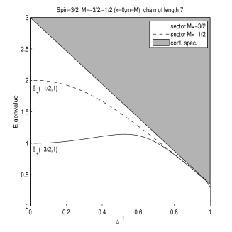
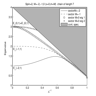
Figure 2. The low-lying spectrum of the XXZ model for $J=\frac{3}{2}$ and $J=2$ for various sectors. Note the two-fold degeneracy for spin $2$ in the sector $M=0$ corresponding to $E_{+}(0,1)=E_{-}(0,1)$. The shaded region contains those eigenvalues which converge to continuous spectrum in the thermodynamic limit. We note that, for $\Delta=1$, the gap vanishes in the thermodynamics limit.

2. Set-up

We study the spin $J$ ferromagnetic XXZ model on the one-dimensional lattice $\mathbb{Z}$. The local Hilbert space for a single site $\alpha$ is $\mathcal{H}_{\alpha}=\mathbb{C}^{2J+1}$ with $J\in\frac{1}{2}\mathbb{N}=\{0,\frac{1}{2},1,\frac{3}{2},2,\dots\}$. We consider the Hilbert space for a finite chain on the sites $[-L,L]=\{-L,-L+1,\dots,+L\}$. This is $\mathcal{H}_{[-L,L]}=\bigotimes_{\alpha=-L}^{L}\mathcal{H}_{\alpha}$. The Hamiltonian of the spin-$J$ XXZ model is

(2.1) $$\begin{gathered}H_{L}(\Delta^{-1})\,=\,\sum_{\alpha=-L}^{L-1}h_{\alpha,\alpha+1}(\Delta^{-1})\,,\\ h_{\alpha,\alpha+1}(\Delta^{-1})\,=\,J^{2}-S_{\alpha}^{3}S_{\alpha+1}^{3}-\Delta^{-1}(S_{\alpha}^{1}S_{\alpha+1}^{1}+S_{\alpha}^{2}S_{\alpha+1}^{2})\,,\end{gathered}$$

where $S_{\alpha}^{1}$,$S_{\alpha}^{2}$ and $S_{\alpha}^{3}$ are the spin-$J$ matrices acting on the site $\alpha$, tensored with the identity operator acting on the other sites. The main parameter of the model is the anisotropy $\Delta>1$ and we get the Ising limit as $\Delta\rightarrow\infty$. It is mathematically more convenient to work with the parameter $\Delta^{-1}$, which we then assume is in the interval $[0,1]$. As we said, $\Delta^{-1}=0$ is the Ising limit, and $\Delta^{-1}=1$ is the isotropic XXX Heisenberg model. It was shown [2, 3, 4, 6] that additional ground states emerge when we add particular boundary terms. Examples of this are the kink and antikink Hamiltonians

(2.2) $$H^{\rm k}_{L}(\Delta^{-1})\ =\,H_{L}(\Delta^{-1})+J\sqrt{1-\Delta^{-2}}\,(S_{-L}^{3}-S_{L}^{3})$$

(2.3) $$H^{\rm ak}_{L}(\Delta^{-1})\, =\,H_{L}(\Delta^{-1})-J\sqrt{1-\Delta^{-2}}\,(S_{-L}^{3}-S_{L}^{3})$$

It is easy to see that the kink and anti-kink Hamiltonians are unitarily equivalent. We will be mainly interested in the kink Hamiltonian with $L\geq 2$. Note that, by a telescoping sum, we can absorb the boundary fields into the local interactions:

(2.4) $$H_{L}^{\rm k}(\Delta^{-1})\,=\,\sum_{\alpha=-L}^{L-1}h^{\rm k}_{\alpha,\alpha+1}(\Delta^{-1})\,,$$

$$h^{\rm k}_{\alpha,\alpha+1}(\Delta^{-1})\,=\,J^{2}-S_{\alpha}^{3}S_{\alpha+1}^{3}-\Delta^{-1}(S_{\alpha}^{1}S_{\alpha+1}^{1}+S_{\alpha}^{2}S_{\alpha+1}^{2})+J\sqrt{1-\Delta^{-2}}\,(S_{\alpha}^{3}-S_{\alpha+1}^{3})$$

The Ising kink Hamiltonian is the result of taking $\Delta\rightarrow\infty$, equivalently setting $\Delta^{-1}=0$, namely it is

(2.5) $$\begin{gathered}H_{L}^{\rm k}(0)\,=\,\sum_{\alpha=-L}^{L-1}h^{\rm k}_{\alpha,\alpha+1}(0)\,,\\ h^{\rm k}_{\alpha,\alpha+1}(0)\,=\,(J^{2}-S_{\alpha}^{3}S_{\alpha+1}^{3})+J(S_{\alpha}^{3}-S_{\alpha+1}^{3})\\ =\,(J+S_{\alpha}^{3})(J-S_{\alpha+1}^{3})\,.\end{gathered}$$

Each of the Hamiltonians introduced above commutes with the total magnetization

$$S^{3}_{\rm tot}\,=\,\sum_{\alpha=-L}^{L}S^{3}_{\alpha}\,.$$

As indicated in the introduction, for each $M\in\{-J(2L+1),\dots,J(2L+1)\}$, the corresponding sector is defined to be the eigenspace of $S^{3}_{\rm tot}$ with eigenvalue $M$; clearly, these are invariant subspaces for all the Hamiltonians introduced above.

The Ising basis is a natural orthonormal basis for $\mathcal{H}_{[-L,L]}$. At each site we have an orthonormal basis of the Hilbert space $\mathcal{H}_{\alpha}$ given by the eigenvectors of $S^{3}_{\alpha}$ and labeled according to their eigenvalues. We will denote this by $S^{3}_{\alpha}|{m}\rangle_{\alpha}=m|{m}\rangle_{\alpha}$ for $m\in[-J,J]$, and $\alpha\in[-L,L]$. Here, and throughout the remainder of the paper, we will use the notation $[-J,J]$ for the set $\{-J,-J+1,\dots,J\}$ as we have done with $[-L,L]$. Finally, there is an orthonormal basis of the entire Hilbert space consisting of simple tensor product vectors: $\bigotimes_{\alpha=-L}^{L}|{m_{\alpha}}\rangle_{\alpha}$.

Also recall that the raising and lowering operators are defined such that

$$S_{\alpha}^{+}|{m}\rangle_{\alpha}\,=\,\begin{cases}\sqrt{J(J+1)-m(m+1)}\,|{m+1}\rangle_{\alpha}&\text{ if $-J\leq m\leq J-1$,}\\ 0&\text{if $m=J$;}\end{cases}$$

$$S_{\alpha}^{-}|{m}\rangle_{\alpha}\,=\,\begin{cases}\sqrt{J(J+1)-m(m-1)}\,|{m-1}\rangle_{\alpha}&\text{ if $-J+1\leq m\leq J$,}\\ 0&\text{if $m=-J$.}\end{cases}$$

A short calculation shows that $S^{1}_{\alpha}$ and $S^{2}_{\alpha}$ are given by $S^{1}_{a}=(S^{+}_{\alpha}+S^{-}_{\alpha})/2$ and $S^{2}_{a}=(S^{+}_{\alpha}-S^{-}_{\alpha})/2i$, and

$$S_{\alpha}^{1}S_{\alpha+1}^{1}+S_{\alpha}^{2}S^{2}_{\alpha+1}\,=\,\frac{1}{2}\left(S_{\alpha}^{+}S_{\alpha+1}^{-}+S_{\alpha}^{-}S_{\alpha+1}^{+}\right)\,.$$

3. Main theorem

Many of the results in this paper concern the kink Hamiltonian given by  (2.4). We will study it as a perturbation of the Ising Hamiltonian  (2.5) in the regime $0<\Delta^{-1}\ll 1$. We denote an Ising configuration as $\vec{m}=(m_{\alpha})_{\alpha=-L}^{L}$, where $m_{\alpha}\in[-J,J]$ for each $\alpha$, and the corresponding basis vector as

$$|{\vec{m}}\rangle\,=\,\bigotimes_{\alpha=-L}^{L}|{m_{\alpha}}\rangle_{\alpha}\,.$$

Observe that the Ising kink Hamiltonian is diagonal with respect to this basis,

(3.1) $$\begin{gathered}H^{\rm k}_{L}(0)\,|{\vec{m}}\rangle\,=\,E^{\rm k}(\vec{m})\,|{\vec{m}}\rangle\,,\quad\text{ where}\\ E^{\rm k}(\vec{m})\,=\,\sum_{\alpha=-L}^{L-1}e^{\rm k}(m_{\alpha},m_{\alpha+1})\quad\text{ and}\\ e^{\rm k}(m_{\alpha},m_{\alpha+1})\,=\,(J+m_{\alpha})(J-m_{\alpha+1})\,.\end{gathered}$$

Since each of the $e^{\rm k}(m_{\alpha},m_{\alpha+1})$ are non-negative, it is easy to see that the ground states of $H^{\rm k}_{L}(0)$ are all of the form

(3.2) $$\Psi_{0}(x,m;L)=|{\vec{m}}\rangle\,,\quad\text{ where }\quad m_{\alpha}\,=\,\begin{cases}-J&\text{ for $-L\leq\alpha\leq x-1$}\\ m&\text{ for $\alpha=x$}\\ J&\text{for $x+1\leq\alpha\leq L$,}\end{cases}$$

with some $x\in[-L,L]$ and $m\in[-J,J]$. Note that the total magnetization corresponding to $\Psi_{0}(x,m;L)$ is $M=-2Jx+m$. As we will verify in Proposition 4.1, it is easy to check that these ground states are unique per sector. We do point out that there is a slight ambiguity in the above labeling scheme, however, since $\Psi_{0}(x-1,-J;L)$ and $\Psi_{0}(x,J;L)$ coincide. Let us consider the following elementary result.

Theorem 3.1.

For $J\in\frac{1}{2}\mathbb{N}$, $L\geq 2$ and $M\in\{-J(2L+1),\dots,J(2L+1)\}$, the eigenspace of $H^{\rm k}_{L}(0)$ corresponding to energy $E=2J$ has dimension at least equal to $2L+1$.

Because of this theorem, we see that, in the $L\to\infty$ limit, the energy $E=2J$ is essential spectrum; an eigenvalue with infinite multiplicity. As our interest is in perturbation theory, it is natural for us to restrict our attention to energies strictly between $0$ and $2J$. We will call the corresponding eigenvectors “low energy excitations”.

We will now describe all the low energy excitations for the Ising kink Hamiltonian. In order to do so, it is convenient to introduce a family of eigenvectors which contains all possible low energy excitations.

Let $x$ be any site away from the boundary, i.e. take $x\in[-L+1,L-1]$, and choose $m\in[-J,J]$. These choices specify a sector $M=-2Jx+m$ and a groundstate $\Psi_{0}(x,m;L)$. If $m<J$, we define the following vectors: For $1\leq n\leq J-m$ set

(3.3) $$\Psi_{n}^{+}(x,m;L)\,=\,|{\vec{m}}\rangle\,,\quad\text{where}\quad m_{\alpha}\,=\,\begin{cases}-J&\text{ if $\alpha\leq x-1$,}\\ m+n&\text{if $\alpha=x$,}\\ J-n&\text{if $\alpha=x+1$,}\\ J&\text{ if $\alpha\geq x+2$.}\end{cases}$$

If $-J<m$, we define the following vectors: For $1\leq n\leq J+m$ set

(3.4) $$\Psi_{n}^{-}(x,m;L)\,=\,|{\vec{m}}\rangle\,,\quad\text{where}\quad m_{\alpha}\,=\,\begin{cases}-J&\text{ if $\alpha\leq x-2$,}\\ -J+n&\text{if $\alpha=x-1$,}\\ m-n&\text{if $\alpha=x$,}\\ J&\text{ if $\alpha\geq x+1$.}\end{cases}$$

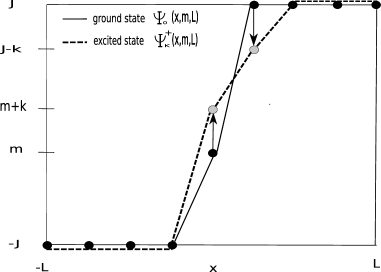
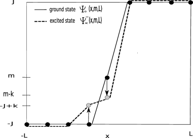
Figure 3. The two kinds of low lying Ising excitations. The left picture belongs to the set $K_{+}(m)$ and the right to the set $K_{-}(m)$.

We call these two sequences of Ising basis vectors the “localized kink excitations”. Clearly, these vectors $\{\Psi_{n}^{\pm}(x,m;L)\}$ have the same total magnetization $M$ and moreover,

(3.5) $$H^{\rm k}_{L}(0)\,\Psi^{\pm}_{n}(x,m;L)\,=\,E_{\pm}(m,n)\,\Psi^{\pm}_{n}(x,m;L),\,\mbox{with }E_{\pm}(m,n)\,=\,n^{2}+(J\pm m)n\,,$$

where $E_{\pm}(m,n)$ has been calculated using (3.1); note that in each case there is only one non-zero term. In Figure 3 we have shown two ground states, in the left and right graphs, as well as two low excitations. These are the schematic diagrams for $\Psi_{0}(x,m)$, in solid in both pictures, and $\Psi_{k}^{+}(x,m)$ and $\Psi_{k}^{-}(x,m)$, in a dashed line, in the left and right, respectively

We now define two sets of labels:

(3.6) $$K_{\pm}(m)\,=\,\{n\,:\,n\in\mathbb{N}\,,\ 1\leq n\leq J\mp m\,,\ E_{\pm}(m,n)<2J\}\,.$$

Depending on $m$ and $J$, neither, one, or both of these sets may be empty. We have the following theorem.

Theorem 3.2.

(1) The low energy excitations of $H^{\rm k}_{L}(0)$ form a subset of the localized kink excitations introduced in (3.3) and (3.4) above.
(2) For $M$ of the form $M=-2Jx+m$ with some $x\in[-L+1,L-1]$ and $m\in[-J,J]$, the set of low energy excitations equals

$$\{\Psi^{+}_{n}(x,m;L)\,:\,n\in K_{+}(m)\}\cup\{\Psi^{-}_{n}(x,m;L)\,:\,n\in K_{-}(m)\}\,.$$

This is a nonempty set except in the following two cases: $J=\frac{1}{2}$, or $J=1$, and $m=0$.
(3) The low energy excitations of $H_{L}^{k}(0)$ are at most two-fold degenerate. The first excitation is simple, except for the case that $J$ is an integer $J>1$, and $M=0$ mod $2J$.

Remark 3.3.

The two-fold degeneracy of the first excited state, guaranteed by part (3) of the theorem, occurs due to the spin flip and reflection symmetry. All other degeneracies with energy $<2J$ occur as follows. Suppose $2J=ab$ for integers $2\leq a\leq b$. In this case, let $m=J-2+a-b$. Then $\Psi_{1}^{+}(x,m;L)$ is degenerate with $\Psi_{a-1}^{-}(x,m;L)$, both with energy $2J-1+a-b$. Similarly, $\Psi_{1}^{-}(x,-m;L)$ is degenerate with $\Psi_{a-1}^{+}(x,-m;L)$ for the same energy.

Next we consider the perturbed Hamiltonian $H^{k}_{L}(\Delta^{-1})$. As is discussed in Section 5.2, each low-lying eigenvalue $E_{\pm}(m,n)$, associated to some $n\in K_{\pm}(m)$, is isolated from the rest of the spectrum by an isolation distance $d_{\pm}(m,n)\geq 1$, independent of $L$, which is defined by

$$d_{\pm}(m,n)=\inf_{E\in\sigma(H^{k}_{L}(0))\setminus\{E_{\pm}(m,n)\}}|E-E_{\pm}(m,n)|\,.$$

Theorem 3.4.

Let $L\geq 2$, and fix $J\geq\frac{3}{2}$. For any $n\in K_{\pm}(m)$, consider the interval $I=[E_{\pm}(m,n)-d_{\pm}(m,n)/2,E_{\pm}(m,n)+d_{\pm}(m,n)/2]$ about the low lying energy $E_{\pm}(m,n)$. The spectral projection of $H_{L}^{\rm k}(\Delta^{-1})$ onto $I$ is analytic for large enough values of $\Delta$. In particular, the dimension of the spectral projection onto $I$ is constant for this range of $\Delta$.

Remark 3.5.

Our estimates yield a lower bound on $\Delta$ as is provided by (5.39). A slightly worse bound demonstrates that taking $\Delta>18J^{5/2}$ suffices, but we do not expect either estimate to be sharp.

The above theorem confirms the structure of the spectrum shown in Figure 2. Moreover, since our numerical calculations indicate that some of the eigenvalues enter the continous spectrum, we do not expect this type of perturbation theory to work for the entire range of $\Delta^{-1}\in[0,1]$.

4. Proof of Theorems  3.1 and  3.2 (Excitations of the Ising Model)

In this section, we will focus on the Ising kink Hamiltonian $H_{L}^{\rm k}(0)$, as introduced in (2.5), for a fixed $J\in\frac{1}{2}\mathbb{N}$. The ground states can be characterized as follows:

Proposition 4.1.

The ground states of the Ising kink Hamiltonian are all of the form

(4.1) $$\Psi_{0}(x,m;L)\,=|{\vec{m}}\rangle\,,\quad\text{ where }\quad m_{\alpha}\,=\,\begin{cases}-J&\text{ for $\alpha=-L,\dots,x-1$,}\\ m&\text{ for $\alpha=x$,}\\ +J&\text{ for $\alpha=x+1,\dots,L$;}\end{cases}$$

for $x\in[-L,\dots,L]$ and $m\in[-J,J]$. Moreover, there is exactly one ground state in each sector; the total magnetization eigenvalue for $\Psi_{0}(x,m;L)$ is $M=2Jx+m$.

This proposition was already used, implicitly, in setting up Theorem 3.2. Here we prove it.

Proof: Given any Ising configuration $\vec{m}=(m_{\alpha})_{\alpha=-L}^{L}$, equation (3.1) demonstrates that the energy associated to $|{\vec{m}}\rangle$, $E^{\rm k}(\vec{m})$, is the sum of $2L$ non-negative terms. Therefore, the only way to have $E^{\rm k}(\vec{m})=0$ is if all of the summands are $0$. This is the case only if either $m_{\alpha}=-J$ or $m_{\alpha+1}=+J$ for all $\alpha$. Clearly, this is satisfied for the Ising configurations with $m_{\alpha}=-J$ for all $\alpha<x$, $m_{\alpha}=+J$ for all $\alpha>x$, and $m_{x}$ equal to any number in $[-J,J]$. It is equally easy to see that these are all of the ground state configurations: if $\vec{m}$ is a groundstate configuration and for some $x$ we have $m_{x}\neq-J$, then $m_{x+1}=J$, which, by induction, means that $m_{\alpha}=+J$ for all $\alpha>x$. Similar reasoning yields that $m_{\alpha}=-J$ for all $\alpha<x$.

To show that the ground states are unique in each sector, consider the equation $M-m=-2Jx$, subject to the constraints: $M\in\{-J(2L+1),\dots,J(2L+1)\}$, $m\in[-J,J]$, and $x\in[-L,L]$. If $M-J\neq 0$ mod $2J$, then there is a unique pair $(x,m)$ which satisfies this equation. If $M-J=0$ mod $2J$, then there are two possible solutions $(x,J)$ and $(x-1,-J)$ for some $x$. But then, it is trivial to see that $\Psi_{0}(x,J;L)$ and $\Psi_{0}(x-1,-J;L)$ coincide.  

Thus in any sector $M$, there is a unique ground state eigenvector $\Psi_{0}(x,m;L)$ for some choice of $(x,m)$ with $M=-2Jx+m$. We next observe that there are many eigenvectors with eigenvalue $2J$; recall this was the statement of Theorem 3.1.

Proof of Theorem 3.1: First consider the case that $M-J$ is not divisible by $2J$. Then the unique groundstate eigenvector is $\Psi_{0}(x,m;L)$ for some $x\in[-L,L]$ and $-J<m<J$. If $x>-L$, then for each $y\in[-L,x-2]$ consider the Ising configuration $\vec{m}$ with components

$$m_{\alpha}\,=\,\begin{cases}-J&\text{ if $\alpha\leq x-1$ and $\alpha\neq y$;}\\ -J+1&\text{ if $\alpha=y$;}\\ m-1&\text{ if $\alpha=x$;}\\ J&\text{ if $\alpha\geq x+1$.}\end{cases}$$

The total magnetization for the vector $|{\vec{m}}\rangle$ is still $M$. Using the formula (3.1) again, it is easy to check that $e^{\rm k}(m_{y},m_{y+1})=2J$, $e^{\rm k}(m_{\alpha},m_{\alpha+1})=0$ for all $\alpha\neq y$, and therefore, $E^{\rm k}(\vec{m})=2J$. This constitutes $x-1+L$ possible values of $y$; producing at least this many distinct eigenvectors with energy $2J$. Similarly, if $x<L$ then there are $L-x-1$ Ising configurations of the form $\vec{m}$ with components

$$m_{\alpha}\,=\,\begin{cases}-J&\text{ if $\alpha\leq x-1$;}\\ m+1&\text{ if $\alpha=x$;}\\ J-1&\text{ if $\alpha=y$;}\\ J&\text{ if $\alpha\geq x+1$ and $\alpha\neq y$;}\end{cases}$$

corresponding to some $y\in[x+2,L]$. In total, this gives $2L-2$ orthonormal eigenvectors corresponding to eigenvalue $2J$, yielding a lower bound on the dimension of the eigenspace. If $x=-L$ or $L$, then the dimension is increased by at least 1. In the special case where $M-J$ is divisible by $2J$, the eigenvector can be written in two ways as $\Psi_{0}(x,J;L)$ or $\Psi_{0}(x-1,-J;L)$. When constructing excitations for $y$ to the left of the kink, use the first formula above relative to $\Psi_{0}(x,J;L)$. When constructing excitations for $y$ to the right of the kink, use the second formula above relative to $\Psi_{0}(x-1,-J;L)$. Once again, this results in $2L-1$ orthonormal eigenvectors corresponding to eigenvalue $2J$.  

We now claim that any Ising configuration which is neither a ground state nor a localized kink excitation corresponds to an energy that is at least $2J$. This is the content of the following lemma.

Lemma 4.2.

Consider an Ising configuration $\vec{m}=(m_{\alpha})_{\alpha=-L}^{L}$.
(1) If there is any $x\in[-L,L-1]$ such that $m_{x}>m_{x+1}$, then $E^{\rm k}(\vec{m})\geq 2J$.
(2) If there is any $x\in[-L+1,\dots,L-1]$ such that $m_{x-1}>-J$ and $m_{x+1}<J$, then $E^{\rm k}(\vec{m})\geq 2J$.

Proof: (1) It is clear from (3.1) that we need only prove

(4.2) $$J^{2}-m_{x}m_{x+1}+J(m_{x}-m_{x+1})\,=\,e^{\rm k}(m_{x},m_{x+1})\,\geq\,2J.$$

Since $m_{x}>m_{x+1}$, we have that $J(m_{x}-m_{x+1})\geq J$. We need only verify that $J^{2}-m_{x}m_{x+1}\geq J$ to establish the claim. The product of two integers $m_{x},m_{x+1}\in[-J,J]$ is at most equal to $J^{2}$. But this is only attained by $m_{x}=m_{x+1}=\pm J$. Since $m_{x}>m_{x+1}$, we can neither have $m_{x+1}=J$ nor $m_{x}=-J$. The next largest possible value of $m_{x}m_{x+1}$ is $J(J-1)$, and we have verified the claim.

(2) Again, because all terms are nonnegative, it suffices to show that

$$e^{\rm k}(m_{x-1},m_{x})+e^{\rm k}(m_{x},m_{x+1})\,\geq\,2J\,.$$

Using the formula for $e^{\rm k}(\cdot,\cdot)$ and simplifying gives

$$e^{\rm k}(m_{x-1},m_{x})+e^{\rm k}(m_{x},m_{x+1})\,=\,2J^{2}+J(m_{x-1}-m_{x+1})-m_{x}(m_{x-1}+m_{x+1})\,.$$

Since $|m_{x}|\leq J$, we have

$$e^{\rm k}(m_{x-1},m_{x})+e^{\rm k}(m_{x},m_{x+1})\, \geq\,2J^{2}+J(m_{x-1}-m_{x+1})-J|m_{x-1}+m_{x+1}|$$

$$=\,J(2J+m_{x-1}-m_{x+1}-|m_{x-1}+m_{x+1}|)\,.$$

Therefore,

$$e^{\rm k}(m_{x-1},m_{x})+e^{\rm k}(m_{x},m_{x+1})\,\geq\,\begin{cases}2J(J-m_{x+1})&\text{ if $m_{x-1}+m_{x+1}\geq 0$;}\\ 2J(J+m_{x-1})&\text{ if $m_{x-1}+m_{x+1}\leq 0$.}\end{cases}$$

Since $J-m_{x+1}\geq 1$ and $J+m_{x-1}\geq 1$, in either case we have proven the claim.  

Now we can finish the proof of the first main result, Theorem 3.2.

Proof of Theorem 3.2: Part (1) of the theorem is a direct consequence of Lemma 4.2 because the only Ising configurations that do not satisfy condition (1) or (2) of that lemma are the ground state configurations and the localized kink excitations.

To prove part (2), let $M=-2Jx+m$ for some $x\in[-L+1,L-1]$ and $m\in[-J,J]$. We first consider the case that $J\geq 3/2$.

If $J$ is sufficiently large and $|m|\leq J-2$, then $n=1\in K_{\pm}(m)$ as

$$E_{\pm}(m,1)\,=\,1^{2}+(J\pm m)1\,\leq\,1+J+|m|\,<\,2J\,.$$

So, in this case, both $K_{+}(m)$ and $K_{-}(m)$ are nonempty.

Similarly, if $|m|=J-1$, then either

$$E_{+}(-J+1,1)\,=\,1^{2}+(J+(-J+1))1\,=\,2,$$

or

$$E_{-}(J-1,1)\,=\,1^{2}+(J-(J-1))1\,=\,2.$$

Hence, $1\in K_{+}(m)\cup K_{-}(m)$ if $|m|=J-1$ and $J\geq 3/2$.

Lastly, if $|m|=J$, then either

$$E_{+}(-J,1)\,=\,1^{2}+(J+(-J))1\,=\,1,$$

or

$$E_{-}(J,1)\,=\,1^{2}+(J-J)1\,=\,1.$$

Hence, $1\in K_{+}(m)\cup K_{-}(m)$ if $|m|=J-1$ and $J\geq 1$.

We have proved (2) in the case that $J\geq 3/2$. Actually, the last observation above also verifies (2) in the case that $J=1$ and $m=\pm 1$.

Finally, if $J=1$ and $m=0$, then $E_{\pm}(0,1)=1^{2}+(1\pm 0)=2$ and if $J=1/2$, then $E_{\pm}(\mp 1/2,1)=1^{2}+(1/2-1/2)=1$. In both these cases, the set of kink excitations is empty.

We now prove the first part of (3). First, observe that for any $m\in[-J,J]$, $J\pm m\geq 0$ and therefore with $m$ fixed, both $E_{\pm}(m,n)$ are increasing functions of $n$ for $n\geq 0$. Therefore the only degeneracies that can occur for a particular energy $E$ is if $E_{+}(m,n_{1})=E$ and $E_{-}(m,n_{2})=E$ for some integers $n_{1}$ and $n_{2}$. This is obviously at most a two-fold degeneracy.

In order to prove the second part of (3), we will simply prove Remark 3.3. Without loss of generality, suppose $m\geq 0$. Then $E_{+}(m,2)=4+2J+2m>2J$. So the only possibility for $E_{+}(m,n)$ to be less than $2J$ is if $n=1$, which gives the energy $J+m+1$ and an auxiliary condition, namely $J-m\geq 2$. A degeneracy happens only if there is a $p\geq 1$ such that $E_{-}(m,p)=E_{+}(m,1)$. This means

$$p^{2}+(J-m)p=J+m+1\qquad\Longleftrightarrow\qquad(p+1)(p+J-m-1)\,=\,2J\,.$$

Setting $a=p+1$ and $b=p+J-m-1$ (which satisfies $b\geq a$ because $J-m\geq 2$) we have exactly the result claimed. Note that the second part of (3) refers to the first excitation. For $m\geq 0$, the lowest excitation is $E_{-}(m,1)$. This means $p=1$, which implies $m=0$ and therefore $2J$ is even with $J\geq 2$ (because $J-m\geq 2$).

 

5. Proof of the main theorem

The goal of this section is to prove Theorem 3.4. We will do so by analyzing the kink Hamiltonian $H_{L}^{\rm k}(\Delta^{-1})$ as a perturbation of the Ising limit $H_{L}^{\rm k}(0)$. Within the first subsection below, specifically in Theorem 5.3, we prove that the operators which arise in our expansion of $H_{L}^{\rm k}(\Delta^{-1})$ are relatively bounded with respect to $H_{L}^{\rm k}(0)$. In the next subsection, we discuss how the explicit bounds on $\Delta$, those claimed in Theorem 3.4, follow from relative boundedness and basic perturbation theory.

5.1. Relative Boundedness

In this subsection, we will analyze the kink Hamiltonian introduced in (2.4). Recall that this Hamiltonian is written as

(5.1) $$H_{L}^{\rm k}(\Delta^{-1})\,=\,\sum_{\alpha=-L}^{L-1}h^{\rm k}_{\alpha,\alpha+1}(\Delta^{-1})\,,$$

$$h^{\rm k}_{\alpha,\alpha+1}(\Delta^{-1})\,=\,J^{2}-S_{\alpha}^{3}S_{\alpha+1}^{3}-\Delta^{-1}(S_{\alpha}^{1}S_{\alpha+1}^{1}+S_{\alpha}^{2}S_{\alpha+1}^{2})+J\sqrt{1-\Delta^{-2}}\,(S_{\alpha}^{3}-S_{\alpha+1}^{3}).$$

By adding and subtracting terms of the form $J(S_{\alpha}^{3}-S_{\alpha+1}^{3})$ to the local Hamiltonians, we find that

(5.2) $$H_{L}^{\rm k}(\Delta^{-1})=H_{L}^{\rm k}(0)+\Delta^{-1}H_{L}^{(1)}+\left(1-\sqrt{1-\Delta^{-2}}\,\right)H_{L}^{(2)}$$

where

(5.3) $$H_{L}^{(1)}\,=\,-\,\sum_{\alpha=-L}^{L-1}h_{\alpha,\alpha+1}^{(1)}\quad\mbox{ with }\quad h_{\alpha,\alpha+1}^{(1)}\,=\,\frac{1}{2}(S_{\alpha}^{+}S_{\alpha+1}^{-}+S_{\alpha}^{-}S_{\alpha+1}^{+})$$

and

(5.4) $$H_{L}^{(2)}=J(S_{L}^{3}-S_{-L}^{3}).$$

In Theorem 5.3 below, we will show that both $H_{L}^{(1)}$ and $H_{L}^{(2)}$ are relatively bounded perturbations of $H_{L}^{\rm k}(0)$. To prove such estimates, we will use the following lemma several times.

Lemma 5.1.

Let $A$ and $B$ be self-adjoint $n\times n$ matrices. If $A\geq 0$ and ${\rm Ker}(A)\subset{\rm Ker}(B)$, then there exists a constant $c>0$ for which,

(5.5) $$-cA\,\leq\,B\,\leq\,cA.$$

One may take $c=\frac{\|B\|}{\lambda_{1}}$ where $\lambda_{1}$ denotes the smallest positive eigenvalue of $A$.

Proof: Any vector $\psi\in\mathbb{C}^{n}$ can be written as $\psi=\psi_{0}+\psi_{1}$ where $\psi_{0}\in{\rm Ker}(A)$ and $\psi_{1}\in{\rm Ker}(A)^{\perp}$. Clearly then, $\lambda_{1}\|\psi_{1}\|^{2}\leq\langle\psi,A\psi\rangle$ and therefore

(5.6) $$\left|\langle\psi,B\psi\rangle\right|\,=\,\left|\langle\psi_{1},B\psi_{1}\rangle\right|\,\leq\,\|B\|\,\|\psi_{1}\|^{2}\,\leq\,\frac{\|B\|}{\lambda_{1}}\,\langle\psi,A\psi\rangle,$$

as claimed.  

For our proof of Theorem 5.3, we find it useful to introduce the Ising model without boundary conditions as an auxillary Hamiltonian, i.e.,

$$H_{L}(0)\,=\,\sum_{\alpha=-L}^{L-1}h_{\alpha,\alpha+1}(0)\quad\text{where}\quad h_{\alpha,\alpha+1}(0)\,=\,J^{2}-S_{\alpha}^{3}S_{\alpha+1}^{3}\,.$$

It is easy to prove the next lemma.

Lemma 5.2.

The Ising model without boundary terms is relatively bounded with respect to the Ising kink Hamiltonian. In particular, for any vector $\psi$,

$$\|H_{L}(0)\psi\|\,\leq\,\|H_{L}^{\rm k}(0)\psi\|+2J^{2}\|\psi\|\,.$$

Proof: Consider the terms of the Ising kink Hamiltonian:

(5.7) $$h_{\alpha,\alpha+1}^{\rm k}(0)\,=\,(J+S_{\alpha}^{3})(J-S_{\alpha+1}^{3})\,=\,h_{\alpha,\alpha+1}(0)+J(S_{\alpha}^{3}-S_{\alpha+1}^{3}).$$

Summing on $\alpha$ then, we find that

(5.8) $$H_{L}(0)\,=\,H_{L}^{\rm k}(0)\,+\,J(S_{L}^{3}-S_{-L}^{3}),$$

and therefore, the bound

(5.9) $$\|H_{L}(0)\psi\|\,\leq\,\|H_{L}^{\rm k}(0)\psi\|\,+\,2J^{2}\,\|\psi\|,$$

is clear for any vector $\psi$.  

We now state the relative boundedness result.

Theorem 5.3.

The linear term in the perturbation expansion of $H_{L}^{\rm k}(\Delta^{-1})$, see (5.2), satisfies

(5.10) $$\left\|H_{L}^{(1)}\psi\right\|\,\leq\,\sqrt{J^{2}\,+\,2J^{3}}\,\|H_{L}^{\rm k}(0)\psi\|\,+\,2J^{2}\,\sqrt{J^{2}\,+\,2J^{3}}\,\|\psi\|,$$

for any vector $\psi$. Moreover, we also have that

(5.11) $$\left\|H_{L}^{(2)}\psi\right\|\,\leq\,2J^{2}\left\|\psi\right\|$$

Proof: Using Lemma 5.2, it is clear we need only prove that

(5.12) $$\left\|H_{L}^{(1)}\psi\right\|\,\leq\,\sqrt{J^{2}\,+\,2J^{3}}\left\|H_{L}(0)\psi\right\|.$$

to establish (5.10). To this end, Lemma 5.1 provides an immediate bound on the individual terms of these Hamiltonians. In fact, observe that for any fixed $\alpha$, both $h_{\alpha,\alpha+1}(0)$ and $h_{\alpha,\alpha+1}^{(1)}$ are self-adjoint with $h_{\alpha,\alpha+1}(0)\geq 0$ and

(5.13) $${\rm Ker}\left(h_{\alpha,\alpha+1}(0)\right)\,=\,\left\{|\vec{m}\rangle\,:\,m_{\alpha}=m_{\alpha+1}=\pm J\,\right\}\subset{\rm Ker}\left(h_{\alpha,\alpha+1}^{(1)}\right).$$

It is also easy to see that, for every $\alpha$, the first positive eigenvalue of $h_{\alpha,\alpha+1}(0)$ is $\lambda_{1}=J$, and we have that

(5.14) $$\|h_{\alpha,\alpha+1}^{(1)}\|\,=\,\frac{1}{2}\left\|S_{\alpha}^{+}S_{\alpha+1}^{-}+S_{\alpha}^{-}S_{\alpha+1}^{+}\right\|\,\leq\,J^{2}.$$

An application of Lemma 5.1 yields the operator inequality

(5.15) $$-J\,h_{\alpha,\alpha+1}(0)\,\leq\,h_{\alpha,\alpha+1}^{(1)}\,\leq\,J\,h_{\alpha,\alpha+1}(0),$$

valid for any $\alpha$.

The norm bound we seek to prove will follow from considering products of these local Hamiltonians. For any vector $\psi$, one has that

(5.16) $$\|H_{L}^{(1)}\psi\|^{2}\,=\,\langle\psi,(H_{L}^{(1)})^{2}\psi\rangle\,=\,\sum_{\alpha,\alpha^{\prime}=-L}^{L-1}\langle\psi,h_{\alpha,\alpha+1}^{(1)}\,h_{\alpha^{\prime},\alpha^{\prime}+1}^{(1)}\psi\rangle$$

and

(5.17) $$\|H_{L}(0)\psi\|^{2}\,=\,\langle\psi,(H_{L}(0))^{2}\psi\rangle\,=\,\sum_{\alpha,\alpha^{\prime}=-L}^{L-1}\langle\psi,h_{\alpha,\alpha+1}(0)\,h_{\alpha^{\prime},\alpha^{\prime}+1}(0)\psi\rangle.$$

The arguments we provided above apply equally well to the diagonal terms of (5.16) and (5.17) in the sense that

(5.18) $$-J^{2}\,\left(h_{\alpha,\alpha+1}(0)\right)^{2}\,\leq\,\left(h_{\alpha,\alpha+1}^{(1)}\right)^{2}\,\leq\,J^{2}\,\left(h_{\alpha,\alpha}(0)\right)^{2},$$

is also valid for any $\alpha$. We find a similar bound by considering the terms on the right hand side of (5.16) and (5.17) for which $|\alpha-\alpha^{\prime}|>1$. In this case, each of the operators $h_{\alpha,\alpha+1}(0)$ and $h_{\alpha,\alpha+1}^{(1)}$ commute with both of the operators $h_{\alpha^{\prime},\alpha^{\prime}+1}(0)$ and $h_{\alpha^{\prime},\alpha^{\prime}+1}^{(1)}$. Moreover, we conclude from (5.15) that the operators $g_{\alpha}^{\pm}=J\,h_{\alpha,\alpha+1}(0)\pm h_{\alpha,\alpha+1}^{(1)}$ are non-negative for every $\alpha$. Since all the relevant quantities commute, it is clear that

(5.19) $$0\leq\frac{1}{2}\left(g_{\alpha}^{+}g_{\alpha^{\prime}}^{-}\,+\,g_{\alpha}^{-}g_{\alpha^{\prime}}^{+}\right)\,=\,J^{2}\,h_{\alpha,\alpha+1}(0)h_{\alpha^{\prime},\alpha^{\prime}+1}(0)\,-\,h_{\alpha,\alpha+1}^{(1)}h_{\alpha^{\prime},\alpha^{\prime}+1}^{(1)}.$$

Our observations above imply the following bound

(5.20) $$\left\|H_{L}^{(1)}\psi\right\|^{2}\,-\,J^{2}\,\left\|H_{L}(0)\psi\right\|^{2}\,\leq\,\sum_{\alpha=-L}^{L-2}\left\langle\psi,\left(h_{\alpha,\alpha+1}^{(1)}h_{\alpha+1,\alpha+2}^{(1)}\,+\,h_{\alpha+1,\alpha+2}^{(1)}h_{\alpha,\alpha+1}^{(1)}\right)\psi\right\rangle.$$

In fact, the terms on the right hand side of (5.20) for which either $\alpha^{\prime}=\alpha$ or $|\alpha-\alpha^{\prime}|>1$ are non-positive by (5.18), respectively, (5.19). In the case that $|\alpha-\alpha^{\prime}|=1$, the operators $h_{\alpha,\alpha+1}(0)h_{\alpha^{\prime},\alpha^{\prime}+1}(0)$ are non-negative (since they commute) and hence we may drop these terms; those terms that remain we group as the self-adjoint operators appearing on the right hand side of (5.20) above.

Our estimate is completed by applying Lemma 5.1 one more time. Note that for any $\alpha\in\{-L,\cdots,L-2\}$ the operator $A_{\alpha}=h_{\alpha,\alpha+1}(0)+h_{\alpha+1,\alpha+2}(0)$ is self-adjoint, non-negative, and

(5.21) $${\rm Ker}(A_{\alpha})\,=\,\left\{|\vec{m}\rangle\,:\,m_{\alpha}\,=\,m_{\alpha+1}\,=\,m_{\alpha+2}\,=\,\pm J\right\}\,\subset\,{\rm Ker}(B_{\alpha}),$$

where the self-adjoint operator $B_{\alpha}$ appearing above is given by

(5.22) $$B_{\alpha}=h_{\alpha,\alpha+1}^{(1)}h_{\alpha+1,\alpha+2}^{(1)}\,+\,h_{\alpha+1,\alpha+2}^{(1)}h_{\alpha,\alpha+1}^{(1)}.$$

For each $\alpha$, the first positive eigenvalue of $A_{\alpha}$ is $\lambda_{1}(\alpha)=J$, and it is also easy to see that $\|B_{\alpha}\|\leq 2J^{4}$. Thus, term by term Lemma 5.1 implies that

(5.23) $$\langle\psi,B_{\alpha}\psi\rangle\,\leq\,2J^{3}\,\langle\psi,A_{\alpha}\psi\rangle,$$

from which we conclude that

(5.24) $$\left\|H_{L}^{(1)}\psi\right\|^{2}\,\leq\,\left(J^{2}\,+\,2J^{3}\right)\,\left\|H_{L}(0)\psi\right\|^{2},$$

as claimed in (5.12). We have proved (5.10).

Equation (5.11) follows directly from the easy observation that $\left\|H_{L}^{(2)}\right\|$ is equal to $2J^{2}$.  

5.2. Perturbation theory

In Section 4, we verified that, in any given sector, the spectrum of the Ising kink Hamiltonian, $H_{L}^{\rm k}(0)$, when restricted to the interval $[0,2J)$ consists of only isolated eigenvalues whose multiplicity is at most two. In fact, for the sector $M=-2Jx+m$ these eigenvalues are determined by

(5.25) $$E_{\pm}(m,n)\,=\,n^{2}\,+\,(J\,\pm\,m)n$$

for those values of $n\in\mathbb{N}$ with $E_{\pm}(m,n)<2J$. It is clear from (5.25) that each of these eigenvalues have an isolation distance $d_{\pm}(m,n)>0$ from the rest of the spectrum and that this distance is independent of the length scale $L$.

For our proof of the relative boundedness result in Theorem 5.3, we expanded the Hamiltonian as

(5.26) $$H_{L}^{\rm k}(\Delta^{-1})\,=\,H_{L}^{\rm k}(0)\,+\,\Delta^{-1}H_{L}^{(1)}\,+\,\left(1-\sqrt{1-\Delta^{-2}}\right)H_{L}^{(2)}.$$

Using the first resolvent formula, it is easy to see that

(5.27) $$\left(H_{L}^{\rm k}(\Delta^{-1})-\xi\right)^{-1}\,=\,R(\xi)\,\left[1\,+\,\left(\Delta^{-1}H_{L}^{(1)}\,+\,\left(1-\sqrt{1-\Delta^{-2}}\right)H_{L}^{(2)}\right)\,R(\xi)\,\right]^{-1},$$

where we have denoted the resolvent by $R(\xi)=\left(H_{L}^{\rm k}(0)-\xi\right)^{-1}$, and it is assumed that $\Delta^{-1}$ has been chosen small enough so that

(5.28) $$\left\|\,\left(\Delta^{-1}H_{L}^{(1)}\,+\,\left(1-\sqrt{1-\Delta^{-2}}\right)H_{L}^{(2)}\right)\,R(\xi)\,\right\|\,<\,1.$$

It is clear from sections II.1.3-4 of [18] and chapter I of [19] that the spectral projections corresponding to $H_{L}^{\rm k}(\Delta^{-1})$ can be written as a power series in $\Delta^{-1}$, the coefficients of which being integrals of the resolvent over a fixed contour $\Gamma$. Proving an estimate of the form (5.28) for $\Delta$ large enough, uniformly with respect to $\xi\in\Gamma$, is sufficient to guarantee analyticity of the spectral projections. We verify such a uniform estimate below.

Let $E_{\pm}(m,n)$ be an eigenvalue of $H_{L}^{\rm k}(0)$ with isolation distance $d_{\pm}(m,n)$ as specified above. Denote by $\Gamma$ the circle in the complex plane centered at $E_{\pm}(m,n)$ with radius $d_{\pm}(m,n)/2$. We claim that if

(5.29) $$\Delta\,>\,18J^{5/2},$$

then (5.28) is satisfied uniformly for $\xi\in\Gamma$.

We proved in Theorem 5.3 that for any vector $\psi$,

(5.30) $$\left\|H_{L}^{(1)}\psi\right\|\,\leq\,\sqrt{J^{2}\,+\,2J^{3}}\,\|H_{L}^{\rm k}(0)\psi\|\,+\,2J^{2}\,\sqrt{J^{2}\,+\,2J^{3}}\,\|\psi\|.$$

Applying this bound to vectors $\psi$ of the form $\psi=R(\xi)\phi$ yields a norm estimate on $H_{L}^{(1)}R(\xi)$, i.e.,

(5.31) $$\left\|H_{L}^{(1)}R(\xi)\phi\right\|\,\leq\,\left(\sqrt{J^{2}\,+\,2J^{3}}\,\|H_{L}^{\rm k}(0)R(\xi)\|\,+\,2J^{2}\,\sqrt{J^{2}\,+\,2J^{3}}\,\|R(\xi)\|\right)\|\phi\|.$$

Moreover, since

(5.32) $$\|H_{L}^{\rm k}(0)R(\xi)\|\,\leq\,1\,+\,|\xi|\,\|R(\xi)\|,$$

we have proved that

(5.33) $$\left\|\Delta^{-1}H_{L}^{(1)}R(\xi)\right\|\,\leq\,\Delta^{-1}\sqrt{J^{2}+2J^{3}}\left[1\,+\,(|\xi|\,+\,2J^{2})\,\|R(\xi)\|\,\right].$$

Similar arguments, again using Theorem 5.3, imply that

(5.34) $$\left\|\left(1-\sqrt{1-\Delta^{-2}}\right)H_{L}^{(2)}R(\xi)\right\|\,\leq\,\left(1-\sqrt{1-\Delta^{-2}}\right)\,2J^{2}\,\left\|R(\xi)\right\|.$$

For $\xi\in\Gamma$, the circular contour described above, we have that

(5.35) $$\|R(\xi)\|\,=\,\frac{1}{{\rm dist}(\xi,\sigma(H_{L}^{\rm k}(0)))}\,=\,\frac{2}{d_{\pm}(m,n)},$$

and

(5.36) $$|\xi|\,\leq\,E_{\pm}(m,n)\,+\,d_{\pm}(m,n)/2.$$

We derive a bound of the form (5.28), uniform for $\xi\in\Gamma$, by ensuring $\Delta$ large enough so that

(5.37) $$C_{1}\Delta^{-1}\,+\,C_{2}(1-\sqrt{1-\Delta^{-2}})\,<\,1,$$

where

(5.38) $$C_{1}=\sqrt{J^{2}+2J^{3}}\left[1\,+\,\left(\frac{2E_{\pm}(m,n)}{d_{\pm}(m,n)}\,+\,1\,+\frac{4J^{2}}{d_{\pm}(m,n)}\right)\right]\quad\mbox{ and }\quad C_{2}=\frac{4J^{2}}{d_{\pm}(m,n)}.$$

Explicitly, one finds that the inequality (5.37) is satisfied for all

(5.39) $$\Delta>\frac{C_{1}^{2}+C_{2}^{2}}{C_{2}\sqrt{C_{1}^{2}+2C_{2}-1}+C_{1}-C_{1}C_{2}}$$

Equation (5.29) is a simple sufficient condition for $\Delta$ to satisfy this inequality. This is easy to verify if one first replaces $1-\sqrt{1-\Delta^{-2}}$ by $\Delta^{-2}$ in (5.37).

6. Acknowledgements

This article is based on work supported in part by the U.S. National Science Foundation under Grant # DMS-0605342. J.M. wishes to thank NSF Vigre grant #DMS-0135345. The research of S.S. was supported in part by a U.S. National Science Foundation grant, #DMS-0706927.

References

- [1] O. Bolina, P. Contucci, and B. Nachtergaele, Path Integral Representation for Interface States of the Anisotropic Heisenberg Model, 2000 Phys. Rev. Math. 12 1325
- [2] V. Pasquier and H. Saleur, Common structures between finite systems and conformal field theories through quantum groups, 1990 Nucl Phys B 330 523
- [3] F. C. Alcaraz, S. R. Salinas, and W. F. Wreszinski, Anisotropic ferromagnetic quantum domains, 1995 Phys Rev Lett 75 930
- [4] C.-T. Gottstein and R. F. Werner, Ground states of the infinite q-deformed Heisenberg ferromagnet, arXiv:cond-mat/9501123
- [5] T. Matsui, On ground states of the one-dimensional ferromagnetic model, 1996 Lett Math Phys 37 397
- [6] T. Koma and B. Nachtergaele, The complete set of ground states of the ferromagnetic XXZ chains, 1998, Adv Theor Math Phys 2 533
- [7] N. Datta, T. Kennedy, Instability of interfaces in the antiferromagnetic XXZ chain at zero temperature, 2003, Commun Math Phys 236 477
- [8] T. Matsui, On the absence on non-periodicd ground states for the antiferromagnetic XXZ model, 2005, Commun Math Phys 253 585
- [9] T. Koma, B. Nachtergaele, S. Starr, The spectral gap of the ferromagnetic Spin-J XXZ chain, 2001 Adv Theor Math Phys 5 1047
- [10] P. Caputo, F. Martinelli, Relaxation time of anisotropic simple exclusion processes and quantum Heisenberg models, 2003 Ann Appl Probab 13 691
- [11] P. W. Shor, Polynomial-time algorithms for prime factorization and discrete logarithms on a quantum computer, 1997 SIAM J Comput 26 1484
- [12] M. Nielsen and I. Chuang, 2000 Quantum computation and Quantum Information (Cambridge University Press)
- [13] J. E. Mooij, T. P. Orlando, L. Levitov, L. Tian, Caspar H.van der Wal, Seth Lloyd, Josephson Persistent-Current Qubit, 1999 Science 285 1036
- [14] I. L. Chuang, L. M. K. Vandersypen, X. Zhou, D. W. Leung, S. Lloyd, Experimental Realization of a Quantum Algorithm, 1998 Nature 393 143
- [15] N. Khaneja, R. Brockett, S. J. Glaser, Time optimal control in spin systems, 2001 Phys Rev A 63 032308
- [16] H. Mabuchi and N. Khaneja, Principles and applications of control in quantum systems, 2005 Int J Robust Nonlin 15 647
- [17] A. Galiautdinov, Steering with coupled qubits: A unitary evolution approach, 2007, arXiv:quant-ph/07051784
- [18] Tosio Kato, 1982 Perturbation theory of linear operators (Springer-Verlag)
- [19] B.Simon and M. Reed, 1972 Methods of Modern Mathematical Physics, Vol. IV: Analysis of Operators (Academic press)