Matrix-Lifting Semi-Definite Programming for Decoding in Multiple Antenna Systems

Abstract

This paper presents a computationally efficient decoder for multiple antenna systems. The proposed algorithm can be used for any constellation (QAM or PSK) and any labeling method. The decoder is based on matrix-lifting Semi-Definite Programming (SDP). The strength of the proposed method lies in a new relaxation algorithm applied to the method of [1]. This results in a reduction of the number of variables from $(NK+1)^{2}$ to $(2N+K)^{2}$, where $N$ is the number of antennas and $K$ is the number of constellation points in each real dimension. Since the computational complexity of solving SDP is a polynomial function of the number of variables, we have a significant complexity reduction. Moreover, the proposed method offers a better performance as compared to the best quasi-maximum likelihood decoding methods reported in the literature.

I Introduction

The problem of Maximum Likelihood (ML) decoding in Multi-Input Multi-Output (MIMO) wireless systems is known to be NP-hard. A variety of sub-optimum polynomial time algorithms based on Semi-Definite Programming (SDP) are suggested for MIMO decoding [2, 3, 4, 5, 6, 7, 8, 1, 9]. The first quasi ML decoding methods based on SDP were introduced for PSK signalling [2, 3, 4, 5], offering a near ML performance and a polynomial time worst case complexity. Subsequently, SDP methods were used for decoding of MIMO systems based on QAM constellation [6, 1].

The method presented in [6] is for MIMO systems using 16-QAM, where the structure of constellation is captured by a polynomial constraint. Then, by introducing some slack variables, the constraints are expressed in terms of quadratic polynomials. This method can be generalized for larger constellations at the cost of defining more slack variables, increasing the complexity, and significantly decreasing the performance. The method proposed in [7] is a further relaxation of [6], only utilizing upper and lower bounds on the symbol energy in the relaxation step. There is a very slight degradation in performance compared to [6]; however, its computational complexity is independent of the constellation size for any uniform QAM (order of complexity is cubic). The method in [8] is a further tightening of [7] by appending some inequality conditions that are implicit in the alphabet constraint. Its computational complexity is still less than [6].

In [1], an efficient approximate ML decoder for MIMO systems is developed based on vector lifting SDP. The transmitted vector is expanded as a linear combination (with zero-one coefficients) of all the possible constellation points in each dimension. Using this formulation, the distance minimization in Euclidean space is expressed in terms of a binary quadratic minimization problem. The minimization of this problem is over the set of all binary rank-one matrices with column sums equal to one. Although the algorithm in [1] is a sub-optimal decoding method, it is shown that by adding several extra constraints, it can approach the ML performance. However, implementing the extra constraints increases the computational complexity.

In this paper, we introduce a new algorithm based on matrix-lifting SDP [10, 11] for any constellation (QAM or PSK) and any labeling method. This algorithm is inspired by the method in [1] with an efficient implementation resulting in a better performance and lower computational complexity. In SDP optimization problems, the computational complexity is a polynomial function of the number of variables. Using the proposed method, the number of variables in [1] is decreased from $(NK+1)^{2}$ to $(2N+K)^{2}$, where $N$ is the number of antennas and $K$ is the number of constellation points in each real dimension. In addition to this large reduction in the complexity, simulation results show that the proposed algorithm also outperforms all other known convex quasi-ML decoding methods, e.g. [6, 7, 8].

Following notations are used in the sequel. The space of $N\times K$ (resp. $N\times N$) real matrices is denoted by ${\mathcal{M}}_{N\times K}$ (resp. ${\mathcal{M}}_{N}$), and the space of $N\times N$ symmetric matrices is denoted by ${\mathcal{S}}_{N}$. For a $N\times K$ matrix $\mathbf{X}\in{\mathcal{M}}_{N\times K}$, the $(i,j)$th element is represented by $x_{ij}$, where $1\leq i\leq N,\;1\leq j\leq K$, i.e. ${\bf X}=[x_{ij}]$. We use ${{\rm trace}}(\mathbf{A})$ to denote the trace of a square matrix ${\bf A}$. The space of symmetric matrices is considered with the trace inner product $\langle\mathbf{A},\mathbf{B}\rangle={{\rm trace}}(\mathbf{AB})$. For $\mathbf{A},\mathbf{B}\in{\mathcal{S}}_{N}$, $\mathbf{A}\succeq 0$ (resp. $\mathbf{A}\succ 0$) denotes positive semi-definiteness (resp. positive definiteness), and $\mathbf{A}\succeq\mathbf{B}$ denotes $\mathbf{A}-\mathbf{B}\succeq 0$. For two matrices $\mathbf{A},\mathbf{B}\in{\mathcal{M}}_{N}$, $\mathbf{A}\geq\mathbf{B}$, ($\mathbf{A}>\mathbf{B}$) means $a_{ij}\geq b_{ij}$, $(a_{ij}>b_{ij})$ for all $i,j$. The Kronecker product of two matrices $\mathbf{A}$ and $\mathbf{B}$ is denoted by $\mathbf{A}\otimes\mathbf{B}$. For $\mathbf{X}\in{\mathcal{M}}_{N\times K}$, ${\rm vec}(\mathbf{X})$ denotes the vector in $\mathbb{R}^{NK}$ (real $NK$-dimensional space) that is formed from the columns of the matrix $\mathbf{X}$. For $\mathbf{X}\in{\mathcal{M}}_{N}$, ${\rm diag}(\mathbf{X})$ is a vector of the diagonal elements of $\mathbf{X}$. We use $\mathbf{e}_{N}\in\mathbb{R}^{N}$ (resp. $\mathbf{0}_{N}\in\mathbb{R}^{N}$) to denote the $N\times 1$ vector of all ones (resp. all zeros), $\mathbf{E}_{N\times K}\in{\mathcal{M}}_{N\times K}$ to denote the matrix of all ones, and $\mathbf{I}_{N}$ to denote the $N\times N$ Identity matrix. For $\mathbf{X}\in{\mathcal{M}}_{N\times K}$, the notation $\mathbf{X}(1:i,1:j)$, $i<K$ and $j<N$ denotes the sub-matrix of $\mathbf{X}$ containing the first $i$ rows and the first $j$ columns.

The rest of the paper is organized as follows. The problem formulation is introduced in Section II. Section III is the review of the vector-lifting semi-definite programming presented in [1]. In Section IV, we propose our new algorithm based on matrix-lifting semi-definite programming. We use the geometry of the relaxation to find a projected relaxation which has a better performance. In Section V, we present an optimization method, based on matrix nearness to find the integer solution of the original decoding problem from the relaxed optimization problem. Finally, Section VI conclude the paper with some simulation results.

II Problem Formulation

A MIMO system with $\tilde{M}$ transmit antennas and $\tilde{N}$ receive antennas can be modeled by

$${\bf y}={\bf H}{\bf x}+{\bf n},$$ (1)

where $M=2\tilde{M}$, $N=2\tilde{N}$, ${\bf y}$ is the $M\times 1$ received vector, ${\bf H}$ is $M\times N$ real channel matrix, ${\bf n}$ is $N\times 1$ additive white Gaussian noise vector, and ${\bf x}$ is $N\times 1$ data vector whose components are selected from the set $\{s_{1},\cdots,s_{K}\}$, see [1]. Noting $x_{i}\in\{s_{1},\cdots,s_{K}\}$, for $i=1,\cdots,N$, we have

$$x_{i}=u_{i,1}s_{1}+u_{i,2}s_{2}+\cdots+u_{i,K}s_{K},$$ (2)

where

$$u_{i,j}\in\left\{0,1\right\}\;\;{\rm and}\;\;\sum_{j=1}^{K}u_{i,j}=1,\;\;\forall\,i=1,\cdots,N.$$ (3)

Let

$${\bf U}=\left[\begin{array}[]{ccccccc}u_{1,1}&\cdots&u_{1,K}\\ u_{2,1}&\cdots&u_{2,K}\\ \vdots&\ddots&\vdots\\ u_{N,1}&\cdots&u_{N,K}\end{array}\right] {\bf s}=\left[\begin{array}[]{c}s_{1}\\ \vdots\\ s_{K}\end{array}\right].$$ and (11)

Therefore, the transmitted vector is $\mathbf{x}=\mathbf{U}\mathbf{s}$ where ${\bf U}{\bf e}_{K}={\bf e}_{N}$.

At the receiver, the ML decoding is given by

$$\hat{\mathbf{x}}=\arg\min_{x_{i}\in\{s_{1},\cdots,s_{K}\}}\|\hat{\mathbf{y}}-\mathbf{H}\mathbf{x}\|^{2},$$ (12)

where $\hat{\mathbf{x}}$ is the most likely input vector and $\hat{\mathbf{y}}$ is the received vector. Noting ${\bf x}={\bf Us}$, this problem is equivalent to

$$\min_{\mathbf{Ue}_{K}=\mathbf{e}_{N}}\|\hat{\mathbf{y}}-\mathbf{HUs}\|^{2}\equiv$$

$$\min_{\mathbf{Ue}_{K}=\mathbf{e}_{N}}\mathbf{s}^{T}\mathbf{U}^{T}\mathbf{H}^{T}\mathbf{HUs}-2\hat{\mathbf{y}}^{T}\mathbf{HUs}.$$ (13)

Therefore, the decoding problem can be formulated as

$$\min \mathbf{s}^{T}\mathbf{U}^{T}\mathbf{H}^{T}\mathbf{HUs}-2\hat{\mathbf{y}}^{T}\mathbf{HUs}$$

$$s.t. {\bf Ue}_{K}={\bf e}_{N}$$ (14)

$$u_{i,j}\in\{0,1\}.$$

Let $\mathbf{Q}=\mathbf{H}^{T}\mathbf{H}$, ${\bf S}={\bf ss}^{T}$, $\mathbf{C}=-\mathbf{s\hat{y}}^{T}\mathbf{H}$, and let ${\mathcal{E}}_{N\times K}$ denote the set of all binary matrices in ${\mathcal{M}_{N\times K}}$ with row sums equal to one, i.e.

$${\mathcal{E}}_{N\times K}=\left\{{\bf U}\in{\mathcal{M}_{N\times K}}:{\bf U}{\bf e}_{K}={\bf e}_{N},u_{ij}\in\{0,1\}\right\}.$$ (15)

Therefore, the minimization problem (II) is

$$\min {\rm trace}\left({\bf SU}^{T}{\bf QU}+2{\bf CU}\right)$$

$$s.t. {\bf U}\in{\mathcal{E}}_{N\times K}$$ (16)

III Vector-Lifting Semi-Definite Programming

In order to solve the optimization problem (II), the authors in [1] proposed a quadratic vector optimization solution by defining ${\bf u}={\rm vec}({\bf U}^{T}),{\bf U}\in{\mathcal{E}}_{N\times K}$. By using this notation, the objective function is replaced by ${\bf u}^{T}({\bf Q}\otimes{\bf S}){\bf u}+2{\rm vec}({\bf C})^{T}{\bf u}$. Then, the quadratic form is linearized using the vector $\left[\begin{array}[]{c}1\\ {\bf u}\end{array}\right],$ i.e.

$${\bf Z}_{\bf u} = \left[\begin{array}[]{c}1\\ {\bf u}\end{array}\right]\left[\begin{array}[]{cc}1&{\bf u}^{T}\end{array}\right]$$ (20)

$$= \left[\begin{array}[]{cc}1&{\bf u}^{T}\\ {\bf u}&{\bf u}{\bf u}^{T}\end{array}\right]=\left[\begin{array}[]{cc}1&{\bf u}^{T}\\ {\bf u}&{\bf X}\end{array}\right],$$ (25)

where ${\bf X}={\bf u}{\bf u}^{T}$ and it is relaxed to ${\bf X}\succeq{\bf u}{\bf u}^{T}$, or equivalently, by the Schur complement, to the lifted constraint $\left[\begin{array}[]{cc}1&{\bf u}^{T}\\ {\bf u}&{\bf X}\end{array}\right]\succeq 0.$ Note that this matrix is selected from the set

$${\mathcal{F}}:={\rm conv}\left\{{\bf Z}_{\bf u}:{\bf u}={\rm vec}({\bf U}^{T}),~{}{\bf U}\in{\mathcal{E}}_{N\times K}\right\},$$ (26)

where ${\rm conv(.)}$ denotes the convex hull of a set. Therefore, the decoding problem using vector lifting semi-definite programming can be represented by

$${\rm trace} \left[\begin{array}[]{cc}0&{\rm vec}({\bf C})^{T}\\ {\rm vec}({\bf C})&\mathbf{Q}\otimes\mathbf{S}\end{array}\right]\left[\begin{array}[]{cc}1&{\bf u}^{T}\\ {\bf u}&{\bf X}\end{array}\right]$$ (31)

$$s.t. \left[\begin{array}[]{cc}1&{\bf u}^{T}\\ {\bf u}&{\bf X}\end{array}\right]\in\mathcal{F},$$ (34)

which can be solved by SDP technique.

Note that in (31), the optimization parameter is a matrix in $\mathcal{S}_{NK+1}$, which has $(NK+1)^{2}$ variables. In the following, we reduce the number of optimization variables by exploiting the matrix structure of ${\bf U}$.

IV Matrix-Lifting Semi-Definite Programming

To keep the matrix ${\bf U}$ in its original form in (II), the idea is to use the constraint ${\bf X}={\bf U}^{T}{\bf U}$ instead of ${\bf X}={\bf u}{\bf u}^{T}$. As a result, the relaxation ${\bf X}\succeq{\bf u}{\bf u}^{T}$ is transformed to ${\bf X}\succeq{\bf U}^{T}{\bf U}$, or equivalently, by the Schur complement, $\left[\begin{array}[]{cc}{\bf I}_{N}&{\bf U}\\ {\bf U}^{T}&{\bf X}\end{array}\right]\succeq 0.$ This is known as matrix-lifting semi-definite programming. Define the new variable ${\bf V}={\bf US}$. Since the matrix ${\bf S}$ is symmetric, the objective function in (II) can be represented as the Quadratic Matrix Program [11]

$${\rm trace} \left(\left[\begin{array}[]{cc}{\bf U}^{T}&{\bf V}^{T}\end{array}\right]\left[\begin{array}[]{cc}{\bf 0}&\frac{1}{2}{\bf Q}\\ \frac{1}{2}{\bf Q}&{\bf 0}\end{array}\right]\left[\begin{array}[]{c}{\bf U}\\ {\bf V}\end{array}\right]+2{\bf CU}\right)$$ (40)

$$= {\rm trace} \left(\left[\begin{array}[]{cc}{\bf 0}&\frac{1}{2}{\bf Q}\\ \frac{1}{2}{\bf Q}&{\bf 0}\end{array}\right]\left[\begin{array}[]{c}{\bf U}\\ {\bf V}\end{array}\right]\left[\begin{array}[]{cc}{\bf U}^{T}&{\bf V}^{T}\end{array}\right]+2{\bf CU}\right)$$ (46)

$$= {\rm trace} \left(\mathcal{L}_{\bf Q}{\bf W}_{\bf U}\right),$$ (47)

where

$$\mathcal{L}=\left[\begin{array}[]{ccc}{\bf 0}&{\bf C}&{\bf 0}\\ {\bf C}^{T}&{\bf 0}&\frac{1}{2}{\bf Q}\\ {\bf 0}&\frac{1}{2}{\bf Q}&{\bf 0}\end{array}\right]$$ (48)

and

$${\bf W}_{\bf U}=\left[\begin{array}[]{ccc}{\bf I}&{\bf U}^{T}&{\bf V}^{T}\\ {\bf U}&{\bf UU}^{T}&{\bf UV}^{T}\\ {\bf V}&{\bf VU}^{T}&{\bf VV}^{T}\end{array}\right].$$ (49)

To linearize ${\bf W}_{\bf U}$, we consider the matrix

$$\left[\begin{array}[]{c}{\bf U}\\ {\bf V}\end{array}\right]\left[\begin{array}[]{cc}{\bf U}^{T}&{\bf V}^{T}\end{array}\right]=\left[\begin{array}[]{cc}{\bf X}&{\bf Y}\\ {\bf Y}&{\bf Z}\end{array}\right],$$ (50)

where ${\bf X,Y,Z}\in\mathcal{S}_{N}$. This equality can be relaxed to

$$\left[\begin{array}[]{cc}{\bf UU}^{T}&{\bf UV}^{T}\\ {\bf VU}^{T}&{\bf VV}^{T}\end{array}\right]-\left[\begin{array}[]{cc}{\bf X}&{\bf Y}\\ {\bf Y}&{\bf Z}\end{array}\right]\preceq 0.$$ (51)

It can be shown that this relaxation is convex in the Löwner partial order and it is equivalent to the linear constraint [10]

$${\bf W}\triangleq\left[\begin{array}[]{ccc}{\bf I}&{\bf U}^{T}&{\bf V}^{T}\\ {\bf U}&{\bf X}&{\bf Y}\\ {\bf V}&{\bf Y}&{\bf Z}\end{array}\right]\succeq 0.$$ (52)

On the other hand, the feasible set in (II) is the set of binary matrices in $\mathcal{M}_{N\times K}$ with row sum equal to one, the set $\mathcal{E}_{N\times K}$ in (15). By relaxing the rank-one constraint for the matrix variable in (40), we have a tractable SDP problem. The feasible set for the objective function in (40) is approximated by

$$\mathcal{F}_{\mathcal{M}}={\rm conv}\left\{{\bf W}_{\bf U}\right. | {\bf U}\in{\mathcal{M}_{N\times K}}:{\bf U}{\bf e}_{K}={\bf e}_{N},$$ (53)

$$\left.u_{ij}\in\{0,1\},\forall i,j;{\bf V}={\bf US}\right\}$$

Therefore, the decoding problem can be represented by

$$\min {\rm trace}\left(\mathcal{L}{\bf W}\right)$$

$$s.t. {\bf W}\in\mathcal{F}_{\mathcal{M}}.$$ (54)

Note that the size of matrix ${\bf W}$ is $(2N+K)\times(2N+K)$, compared to $(NK+1)\times(NK+1)$ in [1]. In SDP optimization problems, the computational complexity is a polynomial function of the number of variables (elements of ${\bf W}$). By the new implementation of (IV), the number of variables in [1] is decreased from $(NK+1)^{2}$ to $(2N+K)^{2}$, resulting in a large reduction in the complexity.

Although the rank constraint in (50) is relaxed, we can still consider some additional linear constraints to further improve the quality of the solution. These constraints are valid for the non-convex rank-constrained decoding problem. However, we force the SDP problem to satisfy these constraints. Consider the auxiliary matrix ${\bf V}$ and the symmetric matrices ${\bf X,Y}$ and ${\bf Z}$ in matrix ${\bf W}$. Since ${\bf U}\in\mathcal{E}_{N\times K}$ and $\sum_{j=1}^{N}u_{ij}^{2}=1,$ it is clear that ${\rm diag}(X)={\bf e}_{N}$. Also, ${\bf Y}$ represents ${\bf USU}^{T}$ and ${\bf Z}$ represents ${\bf US^{2}U}^{T}$. It is easy to show that

$${\rm diag}(\bf Y)={\bf U}{\rm diag}(\bf S) {\rm and} {\rm diag}(\bf Z)={\bf U}{\rm diag}(\bf S^{2}).$$ (55)

Moreover, ${\bf S}={\bf ss}^{T}$ (rank-one matrix) and ${\bf S}^{2}=(\sum_{1=i}^{K}s_{i}^{2}){\bf S}$. Therefore, instead of ${\rm diag}(\bf Z)={\bf U}{\rm diag}(\bf S^{2})$, we have a stronger result for ${\bf Z}$, i.e. ${\bf Z}=(\sum_{1=i}^{K}s_{i}^{2}){\bf Y}$. Therefore, we have

$$\min {\rm trace}\left(\mathcal{L}\left[\begin{array}[]{ccc}{\bf I}&{\bf U}^{T}&{\bf V}^{T}\\ {\bf U}&{\bf X}&{\bf Y}\\ {\bf V}&{\bf Y}&{\bf Z}\end{array}\right]\right)$$ (59)

$$s.t. {\bf Ue}_{K}={\bf e}_{N}\;\;;\;\;{\bf U}\geq 0$$ (64)

$${\bf V}={\bf US}$$

$${\rm diag}({\bf X})={\bf e}_{N}$$

$${\rm diag}(\bf Y)={\bf U}{\rm diag}(\bf S)$$

$${\bf Z}=(\sum_{1=i}^{K}s_{i}^{2}){\bf Y}$$

$$\left[\begin{array}[]{ccc}{\bf I}&{\bf U}^{T}&{\bf V}^{T}\\ {\bf U}&{\bf X}&{\bf Y}\\ {\bf V}&{\bf Y}&{\bf Z}\end{array}\right]\succeq 0$$

$${\bf U,V}\in\mathcal{M}_{N\times K},{\bf X,Y,Z}\in\mathcal{S}_{N}$$

The equation in (55) determines the diagonal elements of ${\bf Y}$. This property is hidden in the special structure of ${\bf U}$, i.e. ${\bf U}\in\mathcal{E}_{N\times K}$. By using this property, we can even add more constraints. The equation ${\bf Y}={\bf USU}^{T}$ implies that $Y_{ij}=S_{kl}$ for some $k$ and $l$. Therefore, the value of $Y_{ij}$ is between the minimum and the maximum elements of ${\bf S}$. In addition, it can be easily shown that in communication applications, ${\bf S}$, ${\bf Y}$, and ${\bf Z}$ are diagonal dominant matrices (since ${\bf s}^{T}{\bf e}_{K}=0$). This property can be also used to add more constraints to improve the quality of the solution. Our studies show that the improvements due to including the above constraints are marginal. Therefore, in the sequel, we focus on the form given in (59) with the following consideration. The objective function in (II) is ${\rm trace}\left({\bf SU}^{T}{\bf QU}+2{\bf CU}\right)$ which is equivalent to ${\rm trace}\left({\bf QU}{\bf SU}^{T}+2{\bf UC}\right)$. Exchanging the role of ${\bf Q}$ and ${\bf S}$ results in two different formulations. Here, the auxiliary variable ${\bf V}$ is defined as ${\bf QU}$. Similarly, the auxiliary variables ${\bf X,Y,}$ and ${\bf Z}$ represents ${\bf U}^{T}{\bf U},{\bf U}^{T}{\bf QU},$ and ${\bf U}^{T}{\bf Q}^{2}{\bf U}$, respectively. Therefore, it is easy to show that the equivalent minimization problem is

$$\min {\rm trace}\left(\left[\begin{array}[]{ccc}{\bf 0}&{\bf C}&{\bf 0}\\ {\bf C}^{T}&{\bf 0}&\frac{1}{2}{\bf S}\\ {\bf 0}&\frac{1}{2}{\bf S}&{\bf 0}\end{array}\right]\left[\begin{array}[]{ccc}{\bf I}&{\bf U}&{\bf V}\\ {\bf U}^{T}&{\bf X}&{\bf Y}\\ {\bf V}^{T}&{\bf Y}&{\bf Z}\end{array}\right]\right)$$ (71)

$$s.t. {\bf Ue}_{K}={\bf e}_{N}\;\;;\;\;{\bf U}\geq 0$$ (76)

$${\bf V}={\bf QU}$$

$${\rm diag}({\bf X})={\bf U}^{T}{\bf e}_{N}\;\;;\;\;X_{ij}=0\;i\neq j$$

$${\bf Ye}_{K}={\bf U}^{T}{\bf Qe}_{N}\;\;;\;\;{\rm trace}({\bf YE}_{K})={\rm trace}({\bf QE}_{N})$$

$${\bf Ze}_{K}={\bf U}^{T}{\bf Q}^{2}{\bf e}_{N}\;\;;\;\;{\rm trace}({\bf ZE}_{K})={\rm trace}({\bf Q}^{2}{\bf E}_{N})$$

$$\left[\begin{array}[]{ccc}{\bf I}&{\bf U}&{\bf V}\\ {\bf U}^{T}&{\bf X}&{\bf Y}\\ {\bf V}^{T}&{\bf Y}&{\bf Z}\end{array}\right]\succeq 0$$

$${\bf U,V}\in\mathcal{M}_{N\times K},{\bf X,Y,Z}\in\mathcal{S}^{K},$$

where the size of the variable matrix is $(2K+N)$. Note that both (59) and (71) are equivalent, however, depending on the structure of the system (values of $N$ and $K$), we can use the one which offers a smaller number of variables. In the following, we focus on (59), which is a better choice for $N\leq K$.

IV-A Geometry of the Relaxation

In this section, we eliminate the constraints defining ${\bf Ue}_{K}={\bf e}_{N}$ by providing a tractable representation of the linear manifold spanned by this constraint. This method is called gradient projection or reduced gradient method [12]. The following lemma is on the representation of matrices having sum of the elements in each row equal to one. This lemma is used in our reduced gradient method.

Lemma 1

[1] Let ${\bf G}=\left[\begin{array}[]{c|c}{\bf I}_{K-1}&-{\bf e}_{K-1}\end{array}\right]\in{\mathcal{M}}_{(K-1)\times K}$ and ${\bf F}=\frac{1}{K}\left({\bf E}_{N\times K}-{\bf E}_{N\times(K-1)}{\bf G}\right)\in{\mathcal{M}}_{N\times K}.$ A matrix ${\bf U}\in\mathcal{M}_{N\times K}$ with the property that the summation of its elements in each row is equal to one, i.e. ${\bf Ue}_{K}={\bf e}_{N}$, can be written as

$${\bf U}={\bf F}+\bf{\hat{U}}{\bf G},$$ (77)

where $\bf{\hat{U}}={\bf U}(1:N,1:(K-1))$.

Corollary 1

$\forall{\bf U}\in{\mathcal{E}}_{N\times K}$, $\exists\hat{\bf U}\in{\mathcal{M}}_{N\times(K-1)}$, $\hat{u}_{ij}\in\{0,1\}$ s.t. ${\bf U}={\bf F}+\bf{\hat{U}}{\bf G}$, where $\bf{\hat{U}}={\bf U}(1:N,1:(K-1))$. Note that the summation of each row of $\bf{\hat{U}}$ is 0 or 1.

Consider the minimization problem (II). By substituting (77), the objective function is

$${\rm trace}\left({\bf SU}^{T}{\bf QU}+2{\bf CU}\right)$$ (78)

$$= {\rm trace}\left({\bf S(F+\hat{U}G)}^{T}{\bf Q(F+\hat{U}G)}+2{\bf C(F+\hat{U}G)}\right)$$

$$= {\rm trace}\left({\bf GSG}^{T}\bf{\hat{U}}^{T}{\bf Q}\bf{\hat{U}}+{\bf GSF}^{T}{\bf Q}\bf{\hat{U}}+{\bf QFSG}^{T}\bf{\hat{U}}^{T}\right.$$

$$\qquad\quad\left.+{\bf GC}\bf{\hat{U}}+{\bf C}^{T}{\bf G}^{T}\bf{\hat{U}}^{T}+2{\bf CF}+{\bf SF}^{T}{\bf QF}\right)$$

$$= {\rm trace}\left(\hat{\mathcal{L}}\bf{W}_{\bf{\hat{U}}}+2{\bf CF}+{\bf SF}^{T}{\bf QF}\right),$$

where

$$\hat{\mathcal{L}} = \left[\begin{array}[]{ccc}{\bf 0}&{\bf GSF}^{T}{\bf Q}+{\bf GC}&{\bf 0}\\ {\bf QFSG}^{T}+{\bf C}^{T}{\bf G}^{T}&{\bf 0}&\frac{1}{2}{\bf Q}\\ {\bf 0}&\frac{1}{2}{\bf Q}&{\bf 0}\end{array}\right],$$ (82)

$${\bf W}_{\bf{\hat{U}}} = \left[\begin{array}[]{ccc}{\bf I}&\bf{\hat{U}}^{T}&\bf{\hat{V}}^{T}\\ \bf{\hat{U}}&\bf{\hat{U}}\bf{\hat{U}}^{T}&\bf{\hat{U}}\bf{\hat{V}}^{T}\\ \bf{\hat{V}}&\bf{\hat{V}}\bf{\hat{U}}^{T}&\bf{\hat{V}}\bf{\hat{V}}^{T}\end{array}\right],$$ (86)

$$\bf{\hat{V}} = \bf{\hat{U}}{\bf GSG}^{T}.$$ (87)

Therefore, (II) can be written as

$$\min {\rm trace}\left(\hat{\mathcal{L}}\bf{W}_{\bf{\hat{U}}}\right)$$

$$s.t. \bf{\hat{U}}={\bf U}(1:N,1:(K-1));\;\;{\bf U}\in{\mathcal{E}}_{N\times K}$$ (88)

$$\bf{\hat{V}}=\bf{\hat{U}}\left({\bf GSG}^{T}\right)$$

Using a similar procedure, we can show that (IV-A) is equivalent to the following reduced matrix-lifting semi-definite programming problem:

$$\min {\rm trace}\left(\hat{\mathcal{L}}\left[\begin{array}[]{ccc}{\bf I}&\bf{\hat{U}}^{T}&\bf{\hat{V}}^{T}\\ \bf{\hat{U}}&\bf{\hat{X}}&\bf{\hat{Y}}\\ \bf{\hat{V}}&\bf{\hat{Y}}&\bf{\hat{Z}}\end{array}\right]\right)$$ (92)

$$s.t. \bf{\hat{U}}{\bf e}_{K-1}\leq{\bf e}_{N}\;\;;\;\;\bf{\hat{U}}\geq 0$$ (97)

$$\bf{\hat{V}}=\bf{\hat{U}}\left({\bf GSG}^{T}\right)$$

$${\rm diag}(\bf{\hat{X}})=\bf{\hat{U}}{\bf e}_{K-1}$$

$${\rm diag}(\bf{\hat{Y}})=\bf{\hat{U}}{\rm diag}\left({\bf GSG}^{T}\right)$$

$$\bf{\hat{Z}}=\left(\sum_{1=i}^{K-1}(s_{i}-s_{K})^{2}\right)\bf{\hat{Y}}$$

$$\left[\begin{array}[]{ccc}{\bf I}&\bf{\hat{U}}^{T}&\bf{\hat{V}}^{T}\\ \bf{\hat{U}}&\bf{\hat{X}}&\bf{\hat{Y}}\\ \bf{\hat{V}}&\bf{\hat{Y}}&\bf{\hat{Z}}\end{array}\right]\succeq 0$$

$$\bf{\hat{U}},\bf{\hat{V}}\in\mathcal{M}_{N\times(K-1)},\bf{\hat{X}},\bf{\hat{Y}},\bf{\hat{Z}}\in\mathcal{S}_{N}$$

Note that this method can also be applied to the equivalent formulation in (71).

IV-B Solving the SDP Problem

The relaxed decoding problems can be solved using Interior-Point Methods (IPMs), which are the most common methods for solving SDP problems of moderate sizes with polynomial computational complexities [13]. There are a large number of IPM-based solvers to handle SDP problems, e.g., DSDP [14], SeDuMi [15], SDPA [16], etc. In our numerical experiments, we use SDPA solver.

In the matrix-lifting SDP optimization problem (59), the rank-constrained matrix ${\bf W}_{\bf u}$ is relaxed to the positive semi-definite matrix ${\bf W}$. Utilizing the rank-constrained property of the variable parameter, the relaxed problem (59) can be solved using a non-linear method, known as the augmented Lagrangian algorithm. This approach can be used for large problem sizes and the complexity can be significantly reduced, while the performance degradation is negligible [17].

V Integer Solution - Matrix Nearness Problem

Solving the relaxed decoding problems results in the solution $\bf{\tilde{U}}$. In general, this matrix is not in $\mathcal{E}_{N\times K}$. The condition ${\bf U}{\bf e}_{K}={\bf e}_{N}$ is satisfied. However, the elements are between 0 and 1. This matrix has to be converted to a 0-1 matrix by finding a matrix in $\mathcal{E}_{N\times K}$ which is nearest to this matrix. Matrix approximation problems typically measure the distance between matrices with a norm. The Frobenius and spectral norms are common choices as they are analytically tractable.

To find the nearest solution in $\mathcal{E}_{N\times K}$ to $\bf{\tilde{U}}$, the solution of the relaxed problem, we solve

$$\min_{{\bf U}\in\;\mathcal{E}_{N\times K}}\|{\bf U}-\bf{\tilde{U}}\|_{\mathds{F}}^{2},$$ (98)

where $\|{\bf A}\|_{\mathds{F}}^{2}$ is the Frobenius norm of the matrix ${\bf A}$ which is defined as $\|{\bf A}\|_{\mathds{F}}^{2}={\rm trace}({\bf AA}^{T})$, and

$$\|{\bf U}-\bf{\tilde{U}}\|_{\mathds{F}}^{2} = {\rm trace}\left(({\bf U}-\bf{\tilde{U}})({\bf U}-\bf{\tilde{U}})^{T}\right)$$ (99)

$$= N-2{\rm trace}(\bf{\tilde{U}}{\bf U}^{T})+{\rm trace}(\bf{\tilde{U}}\bf{\tilde{U}}^{T}).$$

The last equality is due to the fact that for any ${\bf U}\in\mathcal{E}_{N\times K}$, we have ${\rm diag}({\bf UU}^{T})={\bf e}_{N}$, see (59). Therefore, after removing the constants, finding the integer solution is the solution of the following problem:

$$\max_{{\bf U}\in\;\mathcal{E}_{N\times K}}{\rm trace}(\bf{\tilde{U}}{\bf U}^{T})$$ (100)

Consider the maximization problem

$$\max {\rm trace}(\bf{\tilde{U}}{\bf U}^{T})$$

$$s.t. {\bf U}{\bf e}_{K}={\bf e}_{N}$$ (101)

$$0\leq{\bf U}\leq 1,$$

where $\leq$ in the last constraint is element-wise. This problem is a linear programming problem with linear constraints and the optimum solution is a corner point meaning that the constraints are satisfied with equality at the optimum point. In other words, at the optimum point, ${\bf U}\in\mathcal{E}_{N\times K}$. Therefore, to find the solution for (100), we can simply solve the linear problem (V), which is strongly polynomial time. To improve this result, the randomization algorithms, introduced in [1], can be further applied.

VI Simulation Results

We simulate the proposed matrix lifting method (92) for system with $4$ transmit and $4$ receive antennas employing 16-QAM. Fig. 1 shows the performance of the proposed method vs. the performance of the vector lifting method in [1] and the previous known methods in [6, 7, 8]. As it can be seen, the proposed method outperforms all other convex sub-optimal methods.

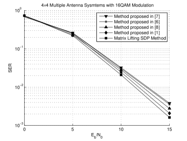
Figure 1: Performance of the proposed matrix lifting SDP method in a MIMO system with $4$ transmit and $4$ receive antennas employing 16-QAM

The worst case complexity of the proposed method solved by IPMs is a polynomial function of the number of antennas (similar to the analysis in [1]). In the optimization problem of (59), where $N\leq K$, the dimension of the matrix variable ${\bf W}$ is $m=O(K)$ and the number of constraints is $p=O(K^{2})$. Similar to [1], it can be easily seen that a solution to (92) can be found in at most $O(K^{5.5})$ arithmetic operations (utilizing the sparsity of the rank-one constraint matrices), where the computational complexity of [1], [6], [8], [7] are $\mathcal{O}(N^{5.5}K^{5.5})$, $\mathcal{O}(N^{6.5}K^{6.5})$, $\mathcal{O}(K^{2}N^{4.5}+K^{3}N^{3.5})$, and $\mathcal{O}(N^{3.5})$ respectively. Note that for the equivalent optimization problem (71), where $K\leq N$, the computational complexity is at most $\mathcal{O}(N^{5.5})$. It must be emphasized that depending on values of $N$ and $K$, we can implement the optimization problem (59) or (71) which results in less computational complexity.

Note that many of the constraints have very simple structures. This property can be used to develop an interior-point optimization algorithm fully exploiting the constraint structures of the problem, thereby getting complexity order better than that of using a general purpose solver such as SeDuMi or SDPA. Moreover, we can further reduce the complexity of the proposed method by implementing the augmented Lagrangian method [17].

References

• [1] A.ย Mobasher, M.ย Taherzadeh, R.ย Sotirov, and A.ย K. Khandani, โ€œA near maximum likelihood decoding algorithm for mimo systems based on semi-definite programming,โ€ to appear in IEEE Trans. on Info. Theory, Nov. 2007.
• [2] B.ย Steingrimsson, T.ย Luo, and K.ย M. Wong, โ€œSoft quasi-maximum-likelihood detection for multiple-antenna wireless channels,โ€ IEEE Transactions on Signal Processing, vol.ย 51, no.ย 11, pp. 2710โ€“ 2719, Nov. 2003.
• [3] B.ย Steingrimsson, Z.ย Q. Luo, and K.ย M. Wong;, โ€œQuasi-ML detectors with soft output and low complexity for PSK modulated MIMO channels,โ€ in 4th IEEE Workshop on Signal Processing Advances in Wireless Communications (SPAWC 2003), 15-18 June 2003, pp. 427 โ€“ 431.
• [4] Z.ย Q. Luo, X.ย Luo, and M.ย Kisialiou, โ€œAn Efficient Quasi-Maximum Likelihood Decoder for PSK Signals,โ€ in ICASSP โ€™03, 2003.
• [5] W.-K. Ma, P.ย C. Ching, and Z.ย Ding, โ€œSemidefinite relaxation based multiuser detection for m-ary psk multiuser systems,โ€ IEEE Trans. on Signal Processing, 2004.
• [6] A.ย Wiesel, Y.ย C. Eldar, and S.ย Shamai, โ€œSemidefinite relaxation for detection of 16-QAM signaling in mimo channels,โ€ IEEE Signal Processing Letters, vol.ย 12, no.ย 9, Sept. 2005.
• [7] N.ย D. Sidiropoulos and Z.-Q. Luo, โ€œA semidefinite relaxation approach to mimo detection for high-order qam constellations,โ€ IEEE SIGNAL PROCESSING LETTERS, vol.ย 13, no.ย 9, Sept. 2006.
• [8] Y.ย Yang, C.ย Zhao, P.ย Zhou, and W.ย Xu, โ€œMimo detection of 16-qam signaling based on semidefinite relaxation,โ€ to appear in IEEE SIGNAL PROCESSING LETTERS, 2007.
• [9] A.ย Mobasher, M.ย Taherzadeh, R.ย Sotirov, and A.ย K. Khandani, โ€œA Near Maximum Likelihood Decoding Algorithm for MIMO Systems Based on Graph Partitioning,โ€ in IEEE International Symposium on Information Theory, Sept. 4-9 2005.
• [10] Y.ย Ding and H.ย Wolkowicz, โ€œA Matrix-lifting Semidefinite Relaxation for the Quadratic Assignment Problem,โ€ Department of Combinatorics & Optimization, University of Waterloo, Tech. Rep. CORR 06-22, 2006.
• [11] A.ย Beck, โ€œQuadratic matrix programming,โ€ SIAM Journal on Optimization, vol.ย 17, no.ย 4, pp. 1224โ€“1238, 2007.
• [12] S.ย Hadley, F.ย Rendl, and H.ย Wolkowicz, โ€œA new lower bound via projection for the quadratic assignment problem,โ€ Math. Oper. Res., vol.ย 17, no.ย 3, pp. 727โ€“739, 1992.
• [13] F.ย Alizadeh, J.-P.ย A. Haeberly, and M.ย Overton, โ€œPrimal-dual interior-point methods for semidefinite programming: Stability, convergence, and numerical results,โ€ SIAM Journal on Optimization, vol.ย 8, no.ย 3, pp. 746โ€“768, 1998.
• [14] S.ย J. Benson and Y.ย Ye, โ€œDSDP5 User Guide The Dual-Scaling Algorithm for Semidefinite Programming,โ€ Mathematics and Computer Science Division, Argonne National Laboratory, Argonne, IL, Tech. Rep. ANL/MCS-TM-255, 2004, available via the WWW site at http://www.mcs.anl.gov/$\sim$benson.
• [15] J.ย Sturm, โ€œUsing sedumi 1.02, a matlab toolbox for optimization over symmetric cones,โ€ Optimization Methods and Software, vol. 11-12, pp. 625โ€“653, 1999.
• [16] M.ย Kojima, K.ย Fujisawa, K.ย Nakata, and M.ย Yamashita, โ€œSDPA(SemiDefinite Programming Algorithm) User s Mannual Version 6.00,โ€ Dept. of Mathematical and Computing Sciences, Tokyo Institute of Technology, 2-12-1 Oh-Okayama, Meguro-ku, Tokyo, 152-0033, Japan, Tech. Rep., 2002, available via the WWW site at http://sdpa.is.titech.ac.jp/SDPA/.
• [17] A.ย Mobasher and A.ย K. Khandani, โ€œMatrix-Lifting SDP for Decoding in Multiple Antenna Systems,โ€ Department of E&CE, University of Waterloo, Tech. Rep. UW-E&CE 2007-06, 2007, available via the WWW site at http://www.cst.uwaterloo.ca/$\sim$amin.