On Zeta Functions and Families of Siegel Modular Forms

Abstract

Let $p$ be a prime, and let $\Gamma=\mathop{\rm Sp}\nolimits_{g}({\mathbb{Z}})$ be the Siegel modular group of genus $g$. We study $p$-adic families of zeta functions and Siegel modular forms.

$L$-functions of Siegel modular forms are described in terms of motivic $L$-functions attached to $\mathop{\rm Sp}\nolimits_{g}$, and their analytic properties are given. Critical values for the spinor $L$-functions and $p$-adic constructions are discussed. Rankin’s lemma of higher genus is established. A general conjecture on a lifting from $\,GSp_{\,2m}\times GSp_{\,2m}$ to $GSp_{\,4m}$ (of genus $g=4m$) is formulated.

Constructions of $p$-adic families of Siegel modular forms are given using Ikeda-Miyawaki constructions.

1 Introduction

The present artical is based on some recent talks of the author, especially the talk in Moscow University on February 2, 2007, for the International conference "Diophantine and Analytical Problems in Number Theory" for 100th birthday of A.O. Gelfond.

Let $\Gamma=\mathop{\rm Sp}\nolimits_{g}({\mathbb{Z}})\subset\mathop{\rm SL}\nolimits_{2g}({\mathbb{Z}})$ be the Siegel modular group of genus $g$. Let $p$ be a prime, $\mathbf{T}(p)=\mathbf{T}(\underbrace{1,\cdots,1}_{g},\underbrace{p,\cdots,p}_{g})$ the Hecke $p$-operator, and $[\mathbf{p}]_{g}=p\mathbf{I}_{2g}=\mathbf{T}(\underbrace{p,\cdots,p}_{2g})$ the scalar Hecke operator for $Sp_{g}$.

We discuss the following topics:

1. $L$-functions of Siegel modular forms

2. Motivic $L$-functions for $\mathop{\rm Sp}\nolimits_{g}$, and their analytic properties

3. Critical values and $p$-adic constructions for the spinor $L$-functions

4. Rankin’s Lemma of higher genus

5. A lifting from $\,GSp_{\,2m}\times GSp_{\,2m}$ to $GSp_{\,4m}$ (of genus $g=4m$)

6. Constructions of $p$-adic families of Siegel modular forms

7. Ikeda-Miyawaki constructions and their $p$-adic versions

2 $L$-functions of Siegel modular forms

The Fourier expansion of a Siegel modular form.

Let $\displaystyle f=\sum_{\mathcal{T}\in B_{n}}a(\mathcal{T})q^{\mathcal{T}}\in\mathcal{M}_{k}^{n}$ be a Siegel modular form of weight $k$ and of genus $n$ on the Siegel upper-half plane $\mathbb{H}_{n}=\{z\in\mathrm{M}_{n}(\mathbb{C})\ |\ \mathrm{Im}(z)>0\}$.

Recal some basic facts about the formal Fourier expansion of $f$, which uses the symbol

$$q^{\mathcal{T}}=\exp(2\pi i\,{\rm tr}({\mathcal{T}}z))=\prod_{i=1}^{n}q_{ii}^{{\mathcal{T}}_{ii}}\prod_{i<j}q_{ij}^{2{\mathcal{T}}_{ij}}$$

$\in\mathbb{C}[\mskip-3.0mu[q_{11},\dots,q_{nn}]\mskip-3.0mu][q_{ij},\ q_{ij}^{-1}]_{i,j=1,\cdots,m}$, where $q_{ij}=\exp(2\pi(\sqrt{-1}z_{i,j}))$, and $\mathcal{T}$ is in the semi-group $B_{n}=\{{\mathcal{T}}={}^{t}{\mathcal{T}}\geq 0|{\mathcal{T}}\hbox{ half-integral}\}.$

Hecke operators and the spherical map

Recall that the local Hecke algebra over ${\mathbb{Z}}$, denoted by $\mathcal{L}_{n,{\mathbb{Z}}}={\mathbb{Z}}[{\mathbf{T}(p)},{\mathbf{T}_{1}(p^{2})},\dotsc,{\mathbf{T}}_{n}(p^{2})]$, is generated by the following $n+1$ Hecke operators

$${\mathbf{T}(p)}:=T(\underbrace{1,\dotsc,1}_{n},\underbrace{p,\dots,p}_{n})\,,$$

$${\mathbf{T}}_{i}(p^{2}):=T(\underbrace{1,\dotsc,1}_{n-i},\underbrace{p,\dotsc,p}_{i},\underbrace{p^{2},\dotsc,p^{2}}_{n-i},\underbrace{p,\dotsc,p}_{i})\,,\,i=1,\dotsc,n$$

${\mathbf{T}}_{n}(p^{2})={[\mathbf{p}]}={[\mathbf{p}]}_{n}=T(\underbrace{p,\dotsc,p}_{2n})=p\/\mathbf{I}_{2n}$ and the spherical map $\Omega:\mathcal{L}_{n,{\mathbb{Q}}}={\mathbb{Q}}[{\mathbf{T}(p)},{\mathbf{T}_{1}(p^{2})},\dotsc,{\mathbf{T}}_{n}(p^{2})]\to{\mathbb{Q}}[x_{0},x_{1},\dotsc,x_{n}]$ is an a certain injective ring morphism.

Satake parameters of an eigenfunction of Hecke operators

Suppose that $f\in{\mathcal{M}}_{k}^{n}$ an eigenfunction of all Hecke operators $f\longmapsto f|T$, $T\in{\mathcal{L}}_{n,p}$ for all primes $p$, hence $f|T=\lambda_{f}(T)f$.

Then all the numbers $\lambda_{f}(T)\in\mathbb{C}$ define a homomorphism $\lambda_{f}:{\mathcal{L}}_{n,p}\longrightarrow\mathbb{C}$ given by a $(n+1)$-tuple of complex numbers $(\alpha_{0},\alpha_{1},\cdots,\alpha_{n})=(\mathbb{C}^{\times})^{n+1}$ (the Satake parameters of $f$), in such a way that

$$\lambda_{f}(T)=\Omega(T)(\alpha_{0},\alpha_{1},\cdots,\alpha_{n}).$$

In particular, one has

$$\lambda_{f}({[\mathbf{p}]})=\alpha_{0}^{2}\alpha_{1}\cdots\alpha_{n}=p^{kn-n(n+1)/2}$$

$$\lambda_{f}({\mathbf{T}(p)})=\Omega({\mathbf{T}(p)})=\alpha_{0}(1+\alpha_{1})\dotsb(1+\alpha_{n})=\sum\limits_{j=0}^{n}\alpha_{0}s_{j}(\alpha_{1},\alpha_{2},\dotsc,\alpha_{n})\,.$$

$L$-functions, functional equation and motives for $\mathrm{Sp}_{n}$ (see [Pa94], [Yosh01])

One defines

• $\displaystyle Q_{f,p}(X)=(1-\alpha_{0}X)\prod_{r=1}^{n}\prod_{1\leq i_{1}<\cdots<i_{r}\leq n}(1-\alpha_{0}\alpha_{i_{1}}\cdots\alpha_{i_{r}}X),$

• $\displaystyle R_{f,p}(X)=(1-X)\prod_{i=1}^{n}(1-\alpha_{i}^{-1}X)(1-\alpha_{i}X)\in\mathbb{Q}[\alpha_{0}^{\pm 1},\cdots,\alpha_{n}^{\pm 1}][X].$

Then the spinor $L$-function $L(Sp(f),s)$ and the standard $L$-function $L(St(f),s,\chi)$ of $f$ (for $s\in\mathbb{C}$, and for all Dirichlet characters) $\chi$ are defined as the Euler products

• $\displaystyle L(Sp(f),s,\chi)=\prod_{p}Q_{f,p}(\chi(p)p^{-s})^{-1}$

• $\displaystyle L(St(f),s,\chi)=\prod_{p}R_{f,p}(\chi(p)p^{-s})^{-1}$

3 Motivic $L$-functions for $\mathop{\rm Sp}\nolimits_{n}$, and their analytic properties

Relations with $L$-functions and motives for $\mathrm{Sp}_{n}$

Following [Pa94] and [Yosh01], these functions are conjectured to be motivic for all $k>n$:

$$L(Sp(f),s,\chi)=L(M(Sp(f))(\chi),s),L(St(f),s)=L(M(St(f))(\chi),s),\mbox{ where}$$

and the motives $M(Sp(f))$ and $M(St(f))$ are pure if $f$ is a genuine cusp form (not coming from a lifting of a smaller genus):

• $M(Sp(f))$ is a motive over $\mathbb{Q}$ with coefficients in $\mathbb{Q}(\lambda_{f}(n))_{n\in\mathbb{N}}$ of rank $2^{n}$, of weight $w=kn-n(n+1)/2$, and of Hodge type $\oplus_{p,q}H^{p,q}$, with

  $$p=(k-i_{1})+(k-i_{2})+\cdots+(k-i_{r}),$$ (3.1)

  $$q=(k-j_{1})+(k-j_{2})+\cdots+(k-i_{s}),\mbox{ where }r+s=n,$$

  $$1\leq i_{1}<i_{2}<\cdots<i_{r}\leq n,1\leq j_{1}<j_{2}<\cdots<j_{s}\leq n,$$

  $$\{i_{1},\cdots,i_{r}\}\cup\{j_{1},\cdots,i_{s}\}=\{1,2,\cdots,n\};$$

• $M(St(f))$ is a motive over $\mathbb{Q}$ with coefficients in $\mathbb{Q}(\lambda_{f}(n))_{n\in\mathbb{N}}$ of rank $2n+1$, of weight $w=0$, and of Hodge type $H^{0,0}\oplus_{i=1}^{n}(H^{-k+i,k-i}\oplus H^{k-i,-k+i})$.

A functional equation

Following general Deligne’s conjecture [De79] on the motivic $L$-functions, the $L$-function satisfy a functional equation determined by the Hodge structure of a motive:

$$\Lambda(Sp(f),kn-n(n+1)/2+1-s)=\varepsilon(f)\Lambda(Sp(f),s),\text{~{}where}$$

$\Lambda(Sp(f),s)=\Gamma_{n,k}(s)L(Sp(f),s),\varepsilon(f)=(-1)^{k2^{n-2}},$
 
$\Gamma_{1,k}(s)=\Gamma_{\mathbb{C}}(s)=2(2\pi)^{-s}\Gamma(s)$, $\Gamma_{2,k}(s)=\Gamma_{\mathbb{C}}(s)\Gamma_{\mathbb{C}}(s-k+2)$, and
$\Gamma_{n,k}(s)=\prod_{p<q}\Gamma_{\mathbb{C}}(s-p)\Gamma^{a_{+}}_{\mathbb{R}}(s-(w/2))\Gamma_{\mathbb{R}}(s+1-(w/2))^{a_{-}}$ for some non-negative integers $a_{+}$ and $a_{-}$, with $a_{+}+a_{-}=w/2$, and $\Gamma_{\mathbb{R}}(s)=\pi^{-s/2}\Gamma(s/2)$.

In particular, for $n=3$ and $k\geq 5$, this conjectural functional equation has the form $\Lambda(Sp(f),s)=\Lambda(Sp(f),3k-5-s)$, where

$$\Lambda(Sp(f),s)=\Gamma_{\mathbb{C}}(s)\Gamma_{\mathbb{C}}(s-k+3)\Gamma_{\mathbb{C}}(s-k+2)\Gamma_{\mathbb{C}}(s-k+1)L(Sp(f),s).$$

For $k\geq 5$ the critical values in the sense of Deligne [De79] are :

$$s=k,\cdots,2k-5.$$

A study of the analytic properties of $L(Sp(f),s)$

(compare with [Vo]).

One could try to use a link between the eigenvalues $\lambda_{f}(T)$ and the Fourier coefficients $a_{f}({\mathcal{T}})$, where $T\in{\mathcal{D}}(\Gamma,S)$ runs through the Hecke operators, and ${\mathcal{T}}\in B_{n}$ runs over half-integral symmetric matrices. It was found by A.N.Andrianov (see [An67]) that

$$D({X})=\sum_{\delta=0}^{\infty}\mathbf{T}(p^{\delta}){X}^{\delta}=\frac{E({X})}{F({X})},$$

where

$$E({X})$$

$$=1-p^{2}\left(\mathbf{T}_{2}(p^{2})+(p^{2}-p+1)(p^{2}+p+1)[\mathbf{p}]_{3}\right){X}^{2}+(p+1)p^{4}\mathbf{T}(p)[\mathbf{p}]_{3}{X}^{3}$$

$$-p^{7}[\mathbf{p}]_{3}\left(\mathbf{T}_{2}(p^{2})+(p^{2}-p+1)(p^{2}+p+1)[\mathbf{p}]_{3}\right){X}^{4}+p^{15}[\mathbf{p}]_{3}^{3}\,{X}^{6}\,\in{\mathcal{L}}_{\mathbb{Z}}[{X}].$$

Computing a formal Dirichlet series

Knowing $E(X)$, one computes the following formal Dirichlet series

$$D_{E}(s)=\sum_{h=1}^{\infty}\mathbf{T}_{E}(h)h^{-s}=\prod_{p}D_{E,p}(p^{-s}),\mbox{ where}$$

$$D_{E,p}(X)=\sum_{\delta=0}^{\infty}\mathbf{T}_{E}(p^{\delta})X^{\delta}=\frac{D_{p}(X)}{E(X)}=\frac{1}{F(X)}\in{\mathcal{D}}(\Gamma,S)[\mskip-3.0mu[X]\mskip-3.0mu].$$

Main identity

For all ${\mathcal{T}}$ one obtains the following identity

$$a_{f}({\mathcal{T}})L(Sp(f),s)=\sum_{h=1}^{\infty}a_{f}(\mathcal{T},E,h)h^{-s},\mbox{ where}$$

$$f|\mathbf{T}_{E}(h)=\sum_{{\mathcal{T}}\in B_{n}}a_{f}(\mathcal{T},E,h)q^{\mathcal{T}}.$$

Indeed, one has

$$f|\mathbf{T}_{E}(h)=\lambda_{f}(\mathbf{T}_{E}(h))f,\mbox{ and }L(Sp(f),s)=\sum_{h=1}^{\infty}\lambda_{f}(\mathbf{T}_{E}(h))h^{-s},\mbox{ hence }$$

$$\sum_{h=1}^{\infty}f|\mathbf{T}_{E}(h)h^{-s}=L(Sp(f),s)\cdot f=\sum_{h=1}^{\infty}\sum_{{\mathcal{T}}\in B_{n}}a_{f}(\mathcal{T},E,h)h^{-s}q^{\mathcal{T}},$$

and it suffices to compare the Fourier coefficients. Such an identity is an unavoidable step in the problem of analytic continuation of $L(Sp(f),s)$ and in the study of its arithmetical implications: one obtains a mean of computing special values out of Fourier coefficients.

For the standard $L$-function $L(St(f),s)$, (see [Pa94], [CourPa], and [Boe-Schm]).

4 Critical values, periods and $p$-adic $L$-functions for $\mathop{\rm Sp}\nolimits_{3}$

Critical values, periods and $p$-adic $L$-functions for $\mathop{\rm Sp}\nolimits_{3}$

A general conjecture by Coates, Perrin-Riou (see [Co-PeRi], [Co], [Pa94]), predicts that for $n=3$ and $k>5$, the motivic function $L(Sp(f),s)$, admits a $p$-adic analogue. Let us fix an embedding $i_{p}:\overline{\mathbb{Q}}\to{\mathbb{C}}_{p}=\widehat{\overline{\mathbb{Q}}}_{p}$, and let $\alpha_{0}(p)$ be an inverse root of $Q_{f,p}$ with the smallest $p$-valuation.

• The Panchishkin condition (see [Ha-Li-Sk], [Pa94], [PaAnnIF94]) for the existence of bounded $p$-adic $L$-functions in this case takes the form ${\rm ord}_{p}(\alpha_{0}(p))=0$ ($\alpha_{0}(p)$ is an inverse root with the smallest $p$-valuation). Recall that this condition says:

  for a pure motive $M$ of rank $d$,
  Newton $p$-polygone at ($d/2$)=Hodge polygone at ($d/2$)

• Otherwise, one obtains $p$-adic $L$-functions of logarithmic growth $o(\log^{h}(\cdot))$ with $h=[2{\rm ord}_{p}(\alpha_{0}(p))]+1$, $2{\rm ord}_{p}(\alpha_{0}(p))$ = the difference
  Newton $p$-Polygone at ($d/2$)–Hodge Polygone at ($d/2$)

For the unitary groups, this condition for the existence of $p$-adic $L$-functions was discussed in [Ha-Li-Sk].

5 Rankin’s Lemma of higher genus

Our next purpose is to evaluate the generating series

$$D^{(1,1)}_{p}(X)=\sum_{\delta=0}^{\infty}T(p^{\delta})\otimes T(p^{\delta})\,X^{\delta}\in\mathcal{L}_{2,{\mathbb{Z}}}\otimes\mathcal{L}_{2,{\mathbb{Z}}}[\mskip-3.0mu[X]\mskip-3.0mu].$$

in terms of Hecke algebra generators $\mathcal{L}_{2,{\mathbb{Z}}}\otimes\mathcal{L}_{2,{\mathbb{Z}}}$:

$${\mathbf{T}(p)}\otimes 1,\quad{\mathbf{T}_{1}(p^{2})}\otimes 1,\quad{[\mathbf{p}]}\otimes 1,$$

$$1\otimes{\mathbf{T}(p)},\quad 1\otimes{\mathbf{T}_{1}(p^{2})},\quad 1\otimes{[\mathbf{p}]}.$$

Theorem 5.1 ([PaVaRnk])

For genus $n=2$, we have the following explicit representation

$$D^{(1,1)}_{p}(X)=\sum_{\delta=0}^{\infty}T(p^{\delta})\otimes T(p^{\delta})\,X^{\delta}=(1-p^{6}{[\mathbf{p}]}\otimes{[\mathbf{p}]}X^{2})\frac{R(X)}{S(X)}\,,\text{~{}where}$$

$$R(X)=1+r_{1}X+\dotsc+r_{12}X^{12},\quad{\text{~{}with~{}~{}}r_{1}=r_{11}=0},$$

$$S(X)=1+s_{1}X+\dotsc+s_{16}X^{16},$$

$$\qquad R(X),S(X)\in\mathcal{L}_{2,{\mathbb{Z}}}\otimes\mathcal{L}_{2,{\mathbb{Z}}}[X],$$

where $r_{i}$ and $s_{i}$ are given in the Appendix of [PaVaRnk]

Here we give the Newton polygons of $R(X)$ and $S(X)$ with respect to powers of $p$ and $X$ (see Figure 1). It follows from our comutation that all slopes are integral.

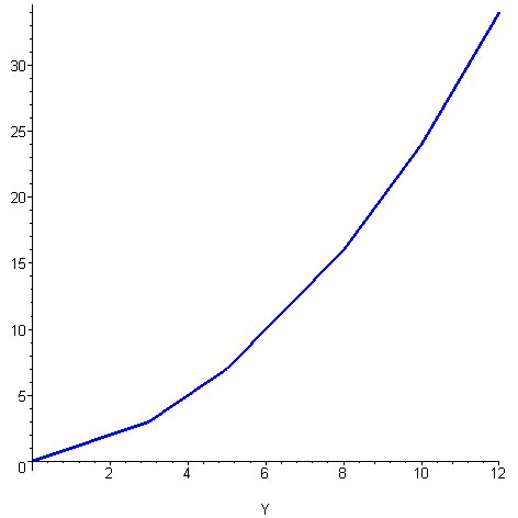
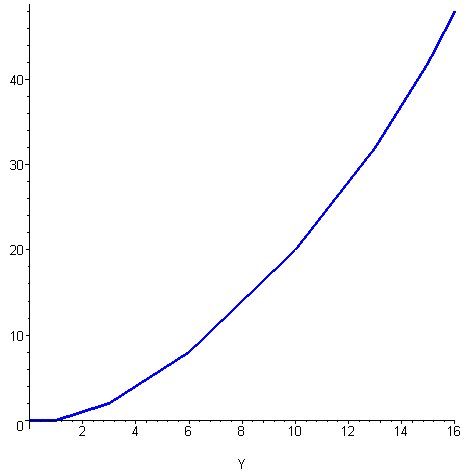
Figure 1: Newton polygons of $R(X)$ and $S(X)$ with respect to powers of $p$ and $X$, of heights 34 and 48, resp.

We hope that these polygons could help to find some geometric objects attached to the polynomials $R(X)$ and $S(X)$, in the spirit of a recent work of C.Faber and G.Van Der Geer, [FVdG].

A half of coefficients: $s_{9},\dotsc,s_{16}$ can be found using this simple functional equation :

$$s_{16-i}=(p^{6}{\mathbf{T}_{2}(p^{2})}\otimes{\mathbf{T}_{2}(p^{2})})^{8-i}s_{i}\ \ \ (i=0,\cdots,8).$$

Proof: Recall that

$$\sum_{\delta=0}^{\infty}\,\Omega^{(n=2)}(T(p^{\delta}))X^{\delta}=\frac{1-\dfrac{x_{0}^{2}x_{1}x_{2}}{p}\,X^{2}}{(1-x_{0}X)\,(1-x_{0}x_{1}X)(1-x_{0}x_{2}X)\,(1-x_{0}x_{1}x_{2}X)\,}$$

From this series it is possible to obtain a formula for ${\Omega}(T(p^{\delta}))$ considering four geometric progressions

$$\sum_{\nu_{1}=0}^{\infty}(x_{0}X)^{\nu_{1}}=\frac{1}{1-x_{0}X},\quad\sum_{\nu_{2}=0}^{\infty}(x_{0}x_{1}X)^{\nu_{2}}=\frac{1}{1-x_{0}x_{1}X}$$

$$\sum_{\nu_{3}=0}^{\infty}(x_{0}x_{2}X)^{\nu_{3}}=\frac{1}{1-x_{0}x_{2}X},\quad\sum_{\nu_{4}=0}^{\infty}(x_{0}x_{1}x_{2}X)^{\nu_{4}}=\frac{1}{1-x_{0}x_{1}x_{2}X}$$

$$\Omega_{x} (T(p^{\delta}))=p^{-1}x_{0}^{\delta}(px_{1}^{(3+\delta)}x_{2}-px_{1}x_{2}^{(3+\delta)}-px_{1}^{(2+\delta)}+px_{2}^{(2+\delta)}-px_{1}^{(3+\delta)}x_{2}^{(2+\delta)}$$

$$+px_{1}^{(2+\delta)}x_{2}^{(3+\delta)}+px_{1}-px_{2}-x_{1}^{(2+\delta)}x_{2}^{2}+x_{1}^{(1+\delta)}x_{2}+x_{1}^{(2+\delta)}x_{2}^{(1+\delta)}-x_{1}^{(1+\delta)}x_{2}^{(2+\delta)}$$

$$+x_{1}^{2}x_{2}^{(2+\delta)}-x_{1}x_{2}^{(1+\delta)}-x_{1}^{2}x_{2}+x_{1}x_{2}^{2})/((1-x_{1})(1-x_{2})(1-x_{1}x_{2})(x_{1}-x_{2}))$$

$$= -p^{-1}x_{0}^{\delta}((1-x_{1}x_{2})(px_{1}-x_{2})x_{1}^{(\delta+1)}+(1-x_{1}x_{2})(x_{1}-px_{2})x_{2}^{(\delta+1)}$$

$$-(1-px_{1}x_{2})(x_{1}-x_{2})(x_{1}x_{2})^{(\delta+1)}-(p-x_{1}x_{2})(x_{1}-x_{2}))/$$

$$\quad((1-x_{1})(1-x_{2})(1-x_{1}x_{2})(x_{1}-x_{2})).$$

Tensor product of local Hecke algebras

We use a second group of variables $y_{0},y_{1},y_{2}$ and $\Omega_{y}$ in order to obtain a tensor product of local Hecke algebras

$$\Omega^{(n)}_{x}\otimes\Omega^{(n)}_{y}:\mathcal{L}_{n,{\mathbb{Q}}}\otimes\mathcal{L}_{n,{\mathbb{Q}}}\to{\mathbb{Q}}[x_{0},x_{1},\dotsc,x_{n};y_{0},y_{1},\dotsc,y_{n}],\text{~{}et}$$

$$\Omega^{(2)}_{y}(T(p^{\delta})):=\Omega^{(2)}_{x}(T(p^{\delta}))|_{x=y}$$

The product of two polynomials $\Omega^{(2)}_{x}(T(p^{\delta}))$ and $\Omega^{(2)}_{y}(T(p^{\delta}))$ is computed straightforward :

$$\Omega {}^{(2)}_{x}(T(p^{\delta}))\cdot\Omega^{(2)}_{y}(T(p^{\delta}))=p^{-2}x_{0}^{\delta}y_{0}^{\delta}(px_{1}^{(3+\delta)}x_{2}-px_{1}^{(2+\delta)}-px_{1}^{(3+\delta)}x_{2}^{(2+\delta)}$$

$$+px_{1}^{(2+\delta)}x_{2}^{(3+\delta)}-px_{1}x_{2}^{(3+\delta)}+px_{2}^{(2+\delta)}+px_{1}-px_{2}-x_{1}^{(2+\delta)}x_{2}^{2}+x_{1}^{(1+\delta)}x_{2}$$

$$+x_{1}^{(2+\delta)}x_{2}^{(1+\delta)}-x_{1}^{(1+\delta)}x_{2}^{(2+\delta)}+x_{1}^{2}x_{2}^{(2+\delta)}-x_{1}x_{2}^{(1+\delta)}-x_{1}^{2}x_{2}+x_{1}x_{2}^{2})$$

$$\times(py_{1}^{(3+\delta)}y_{2}-py_{1}^{(2+\delta)}-py_{1}^{(3+\delta)}y_{2}^{(2+\delta)}+py_{1}^{(2+\delta)}y_{2}^{(3+\delta)}-py_{1}y_{2}^{(3+\delta)}$$

$$+py_{2}^{(2+\delta)}+py_{1}-py_{2}-y_{1}^{(2+\delta)}y_{2}^{2}+y_{1}^{(1+\delta)}y_{2}+y_{1}^{(2+\delta)}y_{2}^{(1+\delta)}$$

$$-y_{1}^{(1+\delta)}y_{2}^{(2+\delta)}+y_{1}^{2}y_{2}^{(2+\delta)}-y_{1}y_{2}^{(1+\delta)}-y_{1}^{2}y_{2}+y_{1}y_{2}^{2})/$$

$$\quad((1-x_{1})(1-x_{2})(1-x_{1}x_{2})(x_{1}-x_{2})(1-y_{1})(1-y_{2})(1-y_{1}y_{2})(y_{1}-y_{2}))$$

Summation of obtained expression give the following result :

$$(\Omega^{(2)}\otimes\Omega^{(2)})(D^{(1,1)}_{p}(X))=\sum_{\delta=0}^{\infty}\,\Omega^{(2)}_{x}(T(p^{\delta}))\cdot\Omega^{(2)}_{y}(T(p^{\delta}))\,X^{\delta}=$$

$$-{\displaystyle\frac{(p\,\mathit{x}_{1}-\mathit{x}_{2})\,(1-p\,\mathit{y}_{1}\,\mathit{y}_{2})\,\mathit{x}_{1}\,\mathit{y}_{1}\,\mathit{y}_{2}}{p^{2}\,(1-\mathit{x}_{1})\,(1-\mathit{x}_{2})\,(\mathit{x}_{1}-\mathit{x}_{2})\,(1-\mathit{y}_{1})\,(1-\mathit{y}_{2})\,(1-\mathit{y}_{1}\,\mathit{y}_{2})\,(1-\mathit{x}_{0}\,\mathit{x}_{1}\,\mathit{y}_{0}\,\mathit{y}_{1}\,\mathit{y}_{2}\,X)}}$$

$$+{\displaystyle\frac{\mathit{x}_{2}\,\mathit{y}_{1}\,(\mathit{x}_{1}-p\,\mathit{x}_{2})\,(p\,\mathit{y}_{1}-\mathit{y}_{2})}{p^{2}\,(1-\mathit{x}_{1})\,(1-\mathit{x}_{2})\,(\mathit{x}_{1}-\mathit{x}_{2})\,(1-\mathit{y}_{1})\,(1-\mathit{y}_{2})\,(\mathit{y}_{1}-\mathit{y}_{2})\,(1-\mathit{x}_{0}\,\mathit{x}_{2}\,\mathit{y}_{0}\,\mathit{y}_{1}\,X)}}$$

$$+{\displaystyle\frac{\mathit{x}_{2}\,\mathit{y}_{2}\,(\mathit{x}_{1}-p\,\mathit{x}_{2})(\mathit{y}_{1}-p\,\mathit{y}_{2})}{p^{2}\,(1-\mathit{x}_{1})\,(1-\mathit{x}_{2})\,(\mathit{x}_{1}-\mathit{x}_{1})\,(1-\mathit{y}_{1})\,(1-\mathit{y}_{2})\,(\mathit{y1}-\mathit{y}_{2})\,(1-\mathit{x}_{0}\,\mathit{y}_{0}\,\mathit{x}_{2}\,\mathit{y}_{2}\,X)}}$$

$$-{\displaystyle\frac{\mathit{x}_{2}\,\mathit{y}_{1}\,\mathit{y}_{2}\,(\mathit{x}_{1}-p\,\mathit{x}_{2})\,(1-p\,\mathit{y}_{1}\,\mathit{y}_{2})}{p^{2}\,(1-\mathit{x}_{1})\,(1-\mathit{x}_{2})\,(\mathit{x}_{1}-\mathit{x}_{2})\,(1-\mathit{y}_{1})\,(1-\mathit{y}_{2})\,(1-\mathit{y}_{1}\,\mathit{y}_{2})\,(1-\mathit{x}_{0}\,\mathit{x}_{2}\,\mathit{y}_{0}\,\mathit{y}_{1}\,\mathit{y}_{2}\,X)}}$$

$$-{\displaystyle\frac{\mathit{x}_{1}\,(p\,\mathit{x}_{1}-\mathit{x}_{2})\,(p-\mathit{y}_{1}\,\mathit{y}_{2})}{p^{2}\,(1-\mathit{x}_{1})\,(1-\mathit{x}_{2})\,(\mathit{x}_{1}-\mathit{x}_{2})\,(1-\mathit{y}_{1})\,(1-\mathit{y}_{2})\,(1-\mathit{y}_{1}\,\mathit{y}_{2})\,(1-\mathit{x}_{0}\,\mathit{x}_{1}\,\mathit{y}_{0}\,X)}}$$

$$-{\displaystyle\frac{\mathit{x}_{1}\,\mathit{x}_{2}\,\mathit{y}_{1}(1-p\,\mathit{x}_{1}\,\mathit{x}_{2})\,(p\,\mathit{y}_{1}-\mathit{y}_{2})}{p^{2}\,(1-\mathit{x}_{1})\,(1-\mathit{x}_{2})\,(1-\mathit{x}_{1}\,\mathit{x}_{2})\,(1-\mathit{y}_{1})\,(1-\mathit{y}_{2})\,(\mathit{y}_{1}-\mathit{y}_{2})\,(1-\mathit{x}_{0}\,\mathit{x}_{1}\,\mathit{x}_{2}\,\mathit{y}_{0}\,\mathit{y}_{1}\,X)}}$$

$$-{\displaystyle\frac{\mathit{x}_{1}\,\mathit{x}_{2}\,\mathit{y}_{2}\,(1-p\,\mathit{x}_{1}\,\mathit{x}_{2})\,(\mathit{y}_{1}-p\,\mathit{y}_{2})}{p^{2}\,(1-\mathit{x}_{1})\,(1-\mathit{x}_{2})\,(1-\mathit{x}_{1}\,\mathit{x}_{2})\,(1-\mathit{y}_{1})\,(1-\mathit{y}_{2})\,(\mathit{y}_{1}-\mathit{y}_{2})\,(1-\mathit{x}_{0}\,\mathit{x}_{1}\,\mathit{x}_{2}\,\mathit{y}_{0}\,\mathit{y}_{2}\,X)}}$$

$$+{\displaystyle\frac{\mathit{y}_{1}\,\mathit{y}_{2}\,(p-\mathit{x}_{1}\,\mathit{x}_{2})\,(1-p\,\mathit{y}_{1}\,\mathit{y}_{2})}{p^{2}\,(1-\mathit{x}_{1})\,(1-\mathit{x}_{2})\,(1-\mathit{x}_{1}\,\mathit{x}_{2})\,(1-\mathit{y}_{1})\,(1-\mathit{y}_{2})\,(1-\mathit{y}_{1}\,\mathit{y}_{2})\,(1-\mathit{x}_{0}\,\mathit{y}_{0}\,\mathit{y}_{1}\,\mathit{y}_{2}\,X)}}$$

$$+{\displaystyle\frac{\mathit{x}_{1}\,\mathit{x}_{2}\,(1-p\,\mathit{x}_{1}\,\mathit{x}_{2})\,(p-\mathit{y}_{1}\,\mathit{y}_{2})}{p^{2}\,(1-\mathit{x}_{1})\,(1-\mathit{x}_{2})\,(1-\mathit{x}_{1}\,\mathit{x}_{2})\,(1-\mathit{y}_{1})\,(1-\mathit{y}_{2})\,(1-\mathit{y}_{1}\,\mathit{y}_{2})\,(1-\mathit{x}_{0}\,\mathit{x}_{1}\,\mathit{x}_{2}\,\mathit{y}_{0}\,X)}}$$

$$-{\displaystyle\frac{\mathit{x}_{1}\,\mathit{y}_{1}\,(p\,\mathit{x}_{1}-\mathit{x}_{2})\,(p\,\mathit{y}_{1}-\mathit{y}_{2})}{p^{2}\,(1-\mathit{x}_{1})\,(1-\mathit{x}_{2})\,(\mathit{x}_{1}-\mathit{x}_{2})\,(1-\mathit{y}_{1})\,(1-\mathit{y}_{2})\,(\mathit{y}_{1}-\mathit{y}_{2})\,(1-\mathit{x}_{0}\,\mathit{x}_{1}\,\mathit{y}_{0}\,\mathit{y}_{1}\,X)}}$$

$$+{\displaystyle\frac{\mathit{x}_{1}\,\mathit{y}_{2}\,(p\,\mathit{x}_{1}-\mathit{x}_{2})\,(\mathit{y}_{1}-p\,\mathit{y}_{2})}{p^{2}\,(1-\mathit{x}_{1})\,(1-\mathit{x}_{2})\,(\mathit{x}_{1}-\mathit{x}_{2})\,(1-\mathit{y}_{1})\,(1-\mathit{y}_{2})\,(\mathit{y}_{1}-\mathit{y}_{2})\,(1-\mathit{x}_{0}\,\mathit{x}_{1}\,\mathit{y}_{0}\,\mathit{y}_{2}\,X)}}$$

$$-{\displaystyle\frac{\mathit{x}_{2}\,(\mathit{x}_{1}-p\,\mathit{x}_{2})\,(p-\mathit{y}_{1}\,\mathit{y}_{2})}{p^{2}\,(1-\mathit{x}_{1})\,(1-\mathit{x}_{2})\,(\mathit{x}_{1}-\mathit{x}_{2})\,(1-\mathit{y}_{1})\,(1-\mathit{y}_{2})\,(1-\mathit{y}_{1}\,\mathit{y}_{2})\,(1-\mathit{x}_{0}\,\mathit{x}_{2}\,\mathit{y}_{0}\,X)}}$$

$$+{\displaystyle\frac{\mathit{x}_{1}\,\mathit{x}_{2}\,\mathit{y}_{1}\,\mathit{y}_{2}\,(1-p\,\mathit{x}_{1}\,\mathit{x}_{2})\,(1-p\,\mathit{y}_{1}\,\mathit{y}_{2})}{p^{2}\,(1-\mathit{x}_{1})\,(1-\mathit{x}_{2})\,(1-\mathit{x}_{1}\,\mathit{x}_{2})\,(1-\mathit{y}_{1})\,(1-\mathit{y}_{2})\,(1-\mathit{y}_{1}\,\mathit{y}_{2})\,(1-\mathit{x}_{0}\,\mathit{x}_{1}\,\mathit{x}_{2}\,\mathit{y}_{0}\,\mathit{y}_{1}\,\mathit{y}_{2}\,X)}}$$

$$+{\displaystyle\frac{(p-\mathit{x}_{1}\,\mathit{x}_{2})\,(p-\mathit{y}_{1}\,\mathit{y}_{2})}{p^{2}\,(1-\mathit{x}_{1})\,(1-\mathit{x}_{2})\,(1-\mathit{x}_{1}\,\mathit{x}_{2})\,(1-\mathit{y}_{1})\,(1-\mathit{y}_{2})\,(1-\mathit{y}_{1}\,\mathit{y}_{2})\,(1-\mathit{x}_{0}\,\mathit{y}_{0}\,X)}}$$

$$-{\displaystyle\frac{\mathit{y}_{1}\,(p-\mathit{x}_{1}\,\mathit{x}_{2})\,(p\,\mathit{y}_{1}-\mathit{y}_{2})}{p^{2}\,(1-\mathit{x}_{1})\,(1-\mathit{x}_{2})\,(1-\mathit{x}_{1}\,\mathit{x}_{2})\,(1-\mathit{y}_{1})\,(1-\mathit{y}_{2})\,(\mathit{y}_{1}-\mathit{y}_{2})\,(1-\mathit{x}_{0}\,\mathit{y}_{0}\,\mathit{y}_{1}\,X)}}$$

$$-{\displaystyle\frac{\mathit{y}_{2}\,(p-\mathit{x}_{1}\,\mathit{x}_{2})\,(\mathit{y}_{1}-p\,\mathit{y}_{2})}{p^{2}\,(1-\mathit{x}_{1})\,(1-\mathit{x}_{2})\,(1-\mathit{x}_{1}\,\mathit{x}_{2})\,(1-\mathit{y}_{1})\,(1-\mathit{y}_{2})\,(\mathit{y}_{1}-\mathit{y}_{2})\,(1-\mathit{x}_{0}\,\mathit{y}_{0}\,\mathit{y}_{2}\,X)}}\,.$$

Properties of the image $(\Omega^{(2)}\otimes\Omega^{(2)})(D^{(1,1)}_{p}(X))$

We checked by an explicit computation that the polynomials, which do not depend of $X$ in the denominator of the image $(\Omega^{(2)}\otimes\Omega^{(2)})(D^{(1,1)}_{p}(X))$, disappear after simplification in the ring ${\mathbb{Q}}[x_{0},x_{1},x_{2},y_{0},y_{1},y_{2}][\mskip-3.0mu[X]\mskip-3.0mu]$, and the common denominator becomes :

$$(1-\mathit{x}_{0}\,\mathit{y}_{0}X)\,(1-\mathit{x}_{0}\,\mathit{y}_{0}\,\mathit{x}_{1}\,X)\,(1-\mathit{x}_{0}\,\mathit{y}_{0}\,\mathit{y}_{1}\,X)\,(1-\mathit{x}_{0}\,\mathit{y}_{0}\,\mathit{x}_{2}\,X)\,(1-\mathit{x}_{0}\,\mathit{y}_{0}\,\mathit{y}_{2}\,X)\,$$

$$(1-\mathit{x}_{0}\,\mathit{y}_{0}\,\mathit{x}_{1}\,\mathit{y}_{1}\,X)\,(1-\mathit{x}_{0}\,\mathit{y}_{0}\,\mathit{x}_{1}\,\mathit{x}_{2}\,X)\,(1-\mathit{x}_{0}\,\mathit{y}_{0}\,\mathit{x}_{1}\,\mathit{y}_{2}\,X)\,(1-\mathit{x}_{0}\,\mathit{y}_{0}\,\mathit{y}_{1}\,\mathit{x}_{2}\,X)\,$$

$$(1-\mathit{x}_{0}\,\mathit{y}_{0}\,\mathit{y}_{1}\,\mathit{y}_{2}\,X)\,(1-\mathit{x}_{0}\,\mathit{y}_{0}\,\mathit{x}_{2}\,\mathit{y}_{2}\,X)\,(1-\mathit{x}_{0}\,\mathit{y}_{0}\,\mathit{x}_{1}\,\mathit{y}_{1}\,\mathit{x}_{2}\,X)\,(1-\mathit{x}_{0}\,\mathit{y}_{0}\,\mathit{x}_{1}\,\mathit{y}_{1}\,\mathit{y}_{2}\,X)\,$$

$$(1-\mathit{x}_{0}\,\mathit{y}_{0}\,\mathit{x}_{1}\,\mathit{x}_{2}\,\mathit{y}_{2}\,X)\,(1-\mathit{x}_{0}\,\mathit{y}_{0}\,\mathit{y}_{1}\,\mathit{x}_{2}\,\mathit{y}_{2}\,X)\,(1-\mathit{x}_{0}\,\mathit{y}_{0}\,\mathit{x}_{1}\,\mathit{y}_{1}\,\mathit{x}_{2}\,\mathit{y}_{2}\,X).$$

Moreover, we found that the numerator consists of the factor $(1-x_{0}^{2}y_{0}^{2}x_{1}y_{1}x_{2}y_{2}X^{2})$ and a polynomial in $X$ of degree $12$ with coefficients in ${\mathbb{Q}}[x_{0},x_{1},x_{2},y_{0},y_{1},y_{2}]$ (the constant term is equal to $1$ and the main term is $p^{-2}x_{0}^{12}y_{0}^{12}x_{1}^{6}x_{2}^{6}y_{1}^{6}y_{2}^{6}X^{12}$). We also found that the factor of degree $12$ does not contain terms of degree $1$ and $11$ in $X$.

It follows that $(\Omega^{(2)}\otimes\Omega^{(2)})(D^{(1,1)}_{p}(X))={\dfrac{(1-x_{0}^{2}y_{0}^{2}x_{1}y_{1}x_{2}y_{2}X^{2})R_{x,y}(X)}{S_{x,y}(X)}}$, where $R_{x,y}(X)=1+r_{2,x,y}X^{2}+\dotsb+r_{10,x,y}X^{10}+r_{12,x,y}X^{12}$ and $S_{x,y}(X)=1+s_{1,x,y}X+\dotsb+s_{16,x,y}X^{16}\in{\mathbb{Q}}[x_{0},x_{1},x_{2},y_{0},y_{1},y_{2},X]$.

Expression through the Hecke operators

Knowing the coefficients of $R_{x,y}(X)$, $S_{x,y}(X)\in{\mathbb{Q}}[x_{0},x_{1},x_{2},y_{0},y_{1},y_{2},X]$ (the images under $\Omega_{x}\otimes\Omega_{y}$) one can reconstruct $R(X)=1+r_{2}X^{2}+\dotsb+r_{10}X^{10}+r_{12}X^{12}$ and $S(X)=1+s_{1}X+\dotsb+s_{16}X^{16}\in\mathcal{L}_{2,{\mathbb{Z}}}\otimes\mathcal{L}_{2,{\mathbb{Z}}}[X]$.

Using the images of the generators

$$\Omega_{x}({\mathbf{T}(p)}^{\lambda_{0}}{\mathbf{T}_{1}(p^{2})}^{\lambda_{1}}{[\mathbf{p}]}^{\lambda_{2}})\Omega_{y}({\mathbf{T}(p)}^{\mu_{0}}{\mathbf{T}_{1}(p^{2})}^{\mu_{1}}{[\mathbf{p}]}^{\mu_{2}}),$$

we build and solve a linear system of undetermined coefficients $K_{\lambda_{0},\lambda_{1},\lambda_{2},\mu_{0},\mu_{1},\mu_{2}}$ expressing all monomials $\Omega_{x}({\mathbf{T}(p)}^{\lambda_{0}}{\mathbf{T}_{1}(p^{2})}^{\lambda_{1}}{[\mathbf{p}]}^{\lambda_{2}})\Omega_{y}({\mathbf{T}(p)}^{\mu_{0}}{\mathbf{T}_{1}(p^{2})}^{\mu_{1}}{[\mathbf{p}]}^{\mu_{2}})$, up to degree $12$ for $R_{x,y}(X)$ ($\leqslant 16$ for $S_{x,y}(X)$) in $x_{0}$ and in $y_{0}$.   $\square$

Comparison with the case of genus $n=1$

The factor $(1-\mathit{x}_{0}^{2}\mathit{y}_{0}^{2}\,\mathit{x}_{1}\mathit{y}_{1}\mathit{x}_{2}\mathit{y}_{2}X^{2})$ of degree $2$ in $X$ is very similar to the one in case of $g=1$ :

$$\sum_{\delta=0}^{\infty}\,{\Omega^{(1)}_{x}}(T(p^{\delta}))\cdot{\Omega^{(1)}_{y}}(T(p^{\delta}))\,X^{\delta}=\sum_{\delta=0}^{\infty}{\displaystyle\frac{\mathit{x}_{0}^{\delta}\,(1-\mathit{x}_{1}^{(1+\delta)})}{1-\mathit{x}_{1}}}\cdot{\displaystyle\frac{\mathit{y}_{0}^{\delta}\,(1-\mathit{y}_{1}^{(1+\delta)})}{1-\mathit{y}_{1}}}X^{\delta}$$

$$={\displaystyle\frac{1}{(1-\mathit{x}_{1})\,(1-\mathit{y}_{1})\,(1-\mathit{x}_{0}\,\mathit{y}_{0}\,X)}}-{\displaystyle\frac{\mathit{y}_{1}}{(1-\mathit{x}_{1})\,(1-\mathit{y}_{1})\,(1-\mathit{x}_{0}\,\mathit{y}_{0}\,\mathit{y}_{1}\,X)}}$$

$$-{\displaystyle\frac{\mathit{x}_{1}}{(1-\mathit{x}_{1})\,(1-\mathit{y}_{1})\,(1-\mathit{x}_{0}\,\mathit{y}_{0}\,\mathit{x}_{1}\,X)}}+{\displaystyle\frac{\mathit{x}_{1}\,\mathit{y}_{1}}{(1-\mathit{x}_{1})\,(1-\mathit{y}_{1})\,(1-\mathit{x}_{0}\,\mathit{y}_{0}\,\mathit{x}_{1}\,\mathit{y}_{1}\,X)}}$$

$$={\displaystyle\frac{1-\mathit{x}_{0}^{2}\,\mathit{y}_{0}^{2}\,\mathit{x}_{1}\,\mathit{y}_{1}\,X^{2}}{(1-\mathit{x}_{0}\,\mathit{y}_{0}\,X)(1-\mathit{x}_{0}\,\mathit{y}_{0}\,\mathit{x}_{1}\,X)\,(1-\mathit{x}_{0}\,\mathit{y}_{0}\,\mathit{y}_{1}\,X)\,{(1-\mathit{x}_{0}\,\mathit{y}_{0}\,\mathit{x}_{1}\,\mathit{y}_{1}\,X)}}}.$$

$$\sum_{\delta=0}^{\infty} \,T(p^{\delta})\otimes T(p^{\delta})\,X^{\delta}=(1-p^{2}{[\mathbf{p}]}\otimes{[\mathbf{p}]}X^{2})\times$$

$$\times(1-{\mathbf{T}(p)}\otimes{\mathbf{T}(p)}X+(p{\mathbf{T}(p)}^{2}\otimes{[\mathbf{p}]}+p{[\mathbf{p}]}\otimes{\mathbf{T}(p)}^{2}-2p^{2}{[\mathbf{p}]}\otimes{[\mathbf{p}]})X^{2}$$

$$-p^{2}{\mathbf{T}(p)}{[\mathbf{p}]}\otimes{\mathbf{T}(p)}{[\mathbf{p}]}X^{3}+p^{4}{[\mathbf{p}]}^{2}\otimes{[\mathbf{p}]}^{2}X^{4})^{-1}\,.$$

6 A lifting from $\,GSp_{\,2m}\times GSp_{\,2m}$ to $GSp_{\,4m}$ of genus $g=4m$

Motive of the Rankin product of genus $n=2$

Let $f$ and $g$ be two Siegel cusp eigenforms of weights $k$ and $l$, $k>l$, and let $M(Sp(f))$ and $M(Sp(g))$ be the (conjectural) spinor motives of $f$ and $g$. Then $M(Sp(f))$ is a motive over $\mathbb{Q}$ with coefficients in $\mathbb{Q}(\lambda_{f}(n))_{n\in\mathbb{N}}$ of rank $4$, of weight $w=2k-3$, and of Hodge type $H^{0,2k-3}\oplus H^{k-2,k-1}\oplus H^{k-1,k-2}\oplus H^{2k-3,0}$, and $M(Sp(g))$ is a motive over $\mathbb{Q}$ with coefficients in $\mathbb{Q}(\lambda_{g}(n))_{n\in\mathbb{N}}$ of rank $4$, of weight $w=2l-3$, and of Hodge type $H^{0,2l-3}\oplus H^{l-2,l-1}\oplus H^{l-1,l-2}\oplus H^{2l-3,0}$.

For another Siegel modular form, an eigenfunction of Hecke operators $g\in\mathcal{M}_{l}^{n}$ consider the corresponding homomorphism $\lambda_{g}:{\mathcal{L}}_{n,p}\longrightarrow\mathbb{C}$ given by its Satake parameters $(\beta_{0},\beta_{1},\cdots,\beta_{n})$ of $g$, and let $\lambda_{f}\otimes\lambda_{g}:{\mathcal{L}}_{n,p}\otimes{\mathcal{L}}_{n,p}\longrightarrow\mathbb{C}$

The tensor product $M(Sp(f))\otimes M(Sp(g))$

is a motive over $\mathbb{Q}$ with coefficients in $\mathbb{Q}(\lambda_{f}(n),\lambda_{g}(n))_{n\in\mathbb{N}}$ of rank $16$, of weight $w=2k+2l-6$, and of Hodge type

$$H^{0,2k+2l-6}\oplus H^{l-2,2k+l-4}\oplus H^{l-1,2k+l-5}\oplus H^{2l-3,2k-3}$$

$$H^{k-2,k+2l-4}\oplus H^{k+l-4,k+l-2}\oplus H_{+}^{k+l-3,k+l-3}\oplus H^{k+2l-5,k-1}$$

$$H^{k-1,k+2l-5}\oplus H_{-}^{k+l-3,k+l-3}\oplus H^{k+l-2,k+l-4}\oplus H^{k+2l-4,k-2}$$

$$H^{2k-3,2l-3}\oplus H^{2k+l-5,l-1}\oplus H^{2k+l-4,l-2}\oplus H^{2k+2l-6,0}.$$

Motivic $L$-functions: analytic properties

Following Deligne’s conjecture [De79] on motivic $L$-functions, applied for a Siegel cusp eigenform $F$ for the Siegel modular group $\mathrm{Sp}_{4}(\mathbb{Z})$ of genus $n=4$ and of weight $k>5$, one has $\Lambda(Sp(F),s)=\Lambda(Sp(F),4k-9-s)$, where

$$\Lambda(Sp(F),s)=\Gamma_{\mathbb{C}}(s)\Gamma_{\mathbb{C}}(s-k+4)\Gamma_{\mathbb{C}}(s-k+3)\Gamma_{\mathbb{C}}(s-k+2)\Gamma_{\mathbb{C}}(s-k+1)$$

$$\times\Gamma_{\mathbb{C}}(s-2k+7)\Gamma_{\mathbb{C}}(s-2k+6)\Gamma_{\mathbb{C}}(s-2k+5)L(Sp(F),s),$$

(compare this functional equation with that given in [An74], p.115).

On the other hand, for $m=2$ and for two cusp eigenforms $f$ and $g$ for $\mathrm{Sp}_{2}(\mathbb{Z})$ of weights $k,l$, $k>l+1$, $\Lambda(Sp(f)\otimes Sp(g),s)=\varepsilon(f,g)\Lambda(Sp(f)\otimes Sp(g),2k+2l-5-s)$, $|\varepsilon(f,g)|=1$, where

$$\Lambda(Sp(f)\otimes Sp(g),s)=\Gamma_{\mathbb{C}}(s)\Gamma_{\mathbb{C}}(s-l+2)\Gamma_{\mathbb{C}}(s-l+1)\Gamma_{\mathbb{C}}(s-k+2)$$

$$\times\Gamma_{\mathbb{C}}(s-k+1)\Gamma_{\mathbb{C}}(s-2l+3)\Gamma_{\mathbb{C}}(s-k-l+2)\Gamma_{\mathbb{C}}(s-k-l+3)$$

$$\times L(Sp(f)\otimes Sp(g),s).$$

We used here the Gauss duplication formula $\Gamma_{\mathbb{C}}(s)=\Gamma_{\mathbb{R}}(s)\Gamma_{\mathbb{R}}(s+1)$. Notice that $a_{+}=a_{-}=1$ in this case, and the conjectural motive $M(Sp(f))\otimes M(Sp(g))$ does not admit critical values.

A holomorphic lifting from $GSp_{2m}\times GSp_{2m}$ to $GSp_{4m}$: a conjecture

Conjecture 6.1 (on a lifting from $\,GSp_{\,2m}\times GSp_{\,2m}$ to $GSp_{\,4m}$)

Let $f$ and $g$ be two Siegel modular forms of genus $2m$ and of weights $k>2m$ and $l=k-2m$. Then there exists a Siegel modular form $F$ of genus $4m$ and of weight $k$ with the Satake parameters $\gamma_{0}=\alpha_{0}\beta_{0},\gamma_{1}=\alpha_{1},\gamma_{2}=\alpha_{2},\cdots,\gamma_{2m}=\alpha_{2m},\gamma_{2m+1}=\beta_{1},\cdots,\gamma_{4m}=\beta_{2m}$ for suitable choices $\alpha_{0},\alpha_{1},\cdots,\alpha_{2m}$ and $\beta_{0},\beta_{1},\cdots,\beta_{2m}$ of Satake’s parameters of $f$ and $g$.

One readily checks that the Hodge types of $M(Sp(f))\otimes M(Sp(g))$ and $M(Sp(F))$ are the same (of rank $2^{4m}$) (it follows from the above description (3.1), and from Künneth’s-type formulas).

An evidence for this version of the conjecture comes from Ikeda-Miyawaki constructions ([Ike01], [Ike06], [Mur02]): let $k$ be an even positive integer, ${h}\in S_{2k}(\Gamma_{1})$ a normalized Hecke eigenform of weight $2k$, $F_{2n}\in S_{k+n}(\Gamma_{2n})$ the Ikeda lift of ${h}$ of genus $2n$ (we assume $k\equiv n\bmod 2$, $n\in\mathbb{N}$).

Next let $f\in S_{k+n+r}(\Gamma_{r})$ be an arbitrary Siegel cusp eigenform of genus $r$ and weight $k+n+r$, with $n,r\geq 1$. If we take $n=m,r=2m$, $k:=k+m$, $k+n+r:=k+3m$, then an example of the validity of this version of the conjecture is given by

$$(f,g)=(f,F_{2m}(h))\mapsto{\cal F}_{{h},f}\in S_{k+3m}(\Gamma_{4m}),$$

$$(f,g)=(f,F_{2m})\in S_{k+3m}(\Gamma_{2m})\times S_{k+m}(\Gamma_{2m}).$$

Another evidence comes from Siegel-Eiseinstein series

$$f=E^{2m}_{k}\mbox{ and }g=E^{2m}_{k-2m}$$

of even genus $2m$ and weights $k$ and $k-2m$: we have then

$$\alpha_{0}=1,\alpha_{1}=p^{k-2m},\cdots,\alpha_{2m}=p^{k-1},$$

$$\beta_{0}=1,\beta_{1}=p^{k-4m},\cdots,\beta_{2m}=p^{k-2m-1},$$

then we have that

$$\gamma_{0}=1,\gamma_{1}=p^{k-4m},\cdots,\gamma_{2m}=p^{k-1},$$

are the Satake parameters of the Siegel-Eisenstein series $F=E^{4m}_{k}$.

Remark 6.2

If we compare the $L$-function of the conjecture (given by the Satake parameters $\gamma_{0}=\alpha_{0}\beta_{0},\gamma_{1}=\alpha_{1},\gamma_{2}=\alpha_{2},\cdots,\gamma_{2m}=\alpha_{2m},\gamma_{2m+1}=\beta_{1},\cdots,\gamma_{4m}=\beta_{2m}$ for suitable choices $\alpha_{0},\alpha_{1},\cdots,\alpha_{2m}$ and $\beta_{0},\beta_{1},\cdots,\beta_{2m}$ of Satake’s parameters of $f$ and $g$), we see that it corresponds to the tensor product of the spinor $L$-functions, and this function is not of the same type as that of the Yoshida’s lifting [Yosh81], which is a certain product of Hecke’s $L$-functions.

We would like to mention in this context Langlands’s functoriality: The denominators of our $L$-series belong to local Langlands $L$-factors (attached to representations of $L$-groups). If we consider the homomorphisms

$${}^{L}GSp_{2m}=GSpin(4m+1)\to GL_{2^{2m}},\ \ {}^{L}GSp_{4m}=GSpin(8m+1)\to GL_{2^{4m}},$$

we see that our conjecture is compatible with the homomorphism of $L$-groups

$$GL_{2^{2m}}\times GL_{2^{2m}}\to GL_{2^{4m}},\ (g_{1},g_{2})\mapsto g_{1}\otimes g_{2},GL_{n}({\mathbb{C}})={}^{L}GL_{n}.$$

However, it is unclear to us if Langlands’s functoriality predicts a holomorphic Siegel modular form as a lift.

7 Constructions of $p$-adic families of Siegel modular forms

Constructing $p$-adic $L$-functions and modular symbols

Together with complex parameter $s$ it is possible to use certain $p$-adic parameters in order to construct $L$-functions and modular symbols. We study such parameters as the twist with Dirichlet character on one hand, and the weight parameter in the theory of families of modular forms on the other. An operation of the twist by a Dirichlet character is a fundamental operation concerning the formal power series, and the $p$-adic variation of such character gives an analytic family of modular forms. One computes the modular symbols related to an automorphic representation $\pi$ of an algebraic group $G$ over a number field, using the twists of automorphic $L$-functions $L(s,\pi\otimes\chi,r)$ with Dirichlet character $\chi$. We represent their special values as integrals giving both complex-analytic and $p$-adic-analytic continuation. We construct analytic families of such $L$-functions in cases $G=\mathrm{GL}_{2}\times\mathrm{GL}_{2}\times\mathrm{GL}_{2}$, $G=\mathrm{GL}_{2}\times\mathrm{GSp}_{2m}$, $G=\mathrm{GSp}_{2m}\times\mathrm{GSp}_{2m}$ using the doubling method and its $p$-adic versions, which expected to work also for overconvergent families of automorphic forms, and already developed in simpler situations $G=\mathrm{GL}_{2}$ by R. Coleman, G. Stevens and others.

A $p$-adic approach

Consider Tate’s field $\mathbb{C}_{p}={\widehat{\overline{\mathbb{Q}}}}_{p}$ for prime number $p$. Let us fix the embedding ${\overline{\mathbb{Q}}}\buildrel i_{p}\over{\hookrightarrow}\mathbb{C}_{p}$ and consider the algebraic numbers as numbers $p$-adic over $i_{p}$. For a $p$-adic family $k{}\mapsto f_{k}=\sum_{n=1}^{\infty}a_{n}(k)q^{n}\in{\overline{\mathbb{Q}}}[\mskip-3.0mu[q]\mskip-3.0mu]\subset\mathbb{C}_{p}[\mskip-3.0mu[q]\mskip-3.0mu]$, the Fourier coefficients $a_{n}(k)$ of $f_{k}$ and one of Satake $p$-parameters $\alpha(k):=\alpha_{p}^{(1)}(k)$ are given by the certain analytical $p$-adic functions $k{}\mapsto a_{n}(k)$ for $(n,p)=1$. The archetypal example of $p$-adic family is given by the Eisenstein series.

$$a_{n}(k)=\sum_{d|n{},{}{}(d,p)=1}d^{k-1},{}{}f_{k}=E_{k},\alpha_{p}^{(1)}(k)=1,\alpha_{p}^{(2)}(k)=p^{k-1}.$$

The existence of the $p$-adic family of cusp forms of positive slope $\sigma>0$ was shown by Coleman. We define the slope $\sigma={\mathrm{ord}}_{p}(\alpha_{p}^{(1)}(k))$ (and ask it to be constant in a $p$-adic neighborhood of weight $k$) An example for $p=7$, $f=\Delta$, $k=12$, $a_{7}=\tau(7)=-7\cdot 2392$, $\sigma=1$ is given by R. Coleman in [CoPB].

Motivation for considering of $p$-adic families

comes from the conjecture of Birch and Swinnerton-Dyer, see [Colm03]. For a cusp eigenform $f=f_{2}$, corresponding to an elliptic curve $E$ by Wiles [Wi95], we consider a family containing $f$. One can try to approach $k=2,s=1$ from the direction, taking $k\to 2$, instead of $s\to 1$, this leads to a formula linking the derivative over $s$ at $s=1$ of the $p$-adic $L$-function with the derivative over $k$ at $k=2$ of the $p$-adic analytic function $\alpha_{p}(k)$, see in [CST98]: ${L^{\prime}_{p,f}(1)=\mathcal{L}_{p}(f)L_{p,f}(1)}$ with $\mathcal{L}_{p}(f)=-2\dfrac{d\alpha_{p}(k)}{dk}\big{|}_{k=2}$. The validity of this formula needs the existence of our two variable $L$-function, constructed in [PaTV].

In order to construct $p$-adic $L$-function of two variables $(k,s)$, the theory of $p$-adic integration is used. The $H$-admissible measures with integer $H$ related to $\sigma$, which appear in this construction, are obtained from $H$-admissible measures with values in various rings of modular forms, in particular nearly holomorphic modular forms. Let us describe a typical example related to differential operators.

Nearly holomorphic modular forms and the method of canonical projection

Let $\mathcal{A}$ be a commutative field. There are several $p$-adic approaches for studying special values of $L$-functions using the method of canonical projection (see [PaTV]). In this method the special values and modular symbols are considered as $\mathcal{A}$-linear forms over spaces of modular forms with coefficients in $\mathcal{A}$. Nearly holomorphic ([ShiAr]) modular forms are certain formal series

$$g=\sum_{n=0}^{\infty}a(n;R)q^{n}\in\mathcal{A}[\mskip-3.0mu[q]\mskip-3.0mu][R]$$

with the property for $\mathcal{A}=\mathbb{C}$, $z=x+iy\in\mathbb{H}$, $R=(4\pi y)^{-1}$, the series converge to a ${\mathcal{C}}^{\infty}$-modular form over $\mathbb{H}$ of given weight $k$ and Dirichlet character $\psi$. The coefficients $a(n;R)$ are polynomials in $\mathcal{A}[R]$ of bounded degree.

Triple products families

give a recent example of families on the algebraic group of higher rank. This aspect was studied by S. Boecherer and A. Panchishkin [Boe-Pa2006]. The triple product with Dirichlet character $\chi$ is defined as a complex $L$-function (Euler product of degree 8)

$$L(f_{1}\otimes f_{2}\otimes f_{3},s,\chi)=\prod_{p\nmid N}L((f_{1}\otimes f_{2}\otimes f_{3})_{p},\chi(p)p^{-s}),$$

where

$$\begin{split}L((f_{1}\otimes f_{2}\otimes f_{3})_{p},X)^{-1}&=\det\left(1_{8}-X\begin{pmatrix}\alpha^{(1)}_{p,1}&0\\ 0&\alpha^{(2)}_{p,1}\end{pmatrix}\otimes\begin{pmatrix}\alpha^{(1)}_{p,2}&0\\ 0&\alpha^{(2)}_{p,2}\end{pmatrix}\otimes\begin{pmatrix}\alpha^{(1)}_{p,3}&0\\ 0&\alpha^{(2)}_{p,3}\end{pmatrix}\right).\end{split}$$

We use the corresponding normalized $L$-function (see [De79], [Co], [Co-PeRi]) :

$$\Lambda(f_{1}\otimes f_{2}\otimes f_{3},s,\chi)=\Gamma_{\mathbb{C}}(s)\Gamma_{\mathbb{C}}(s-k_{3}+1)\Gamma_{\mathbb{C}}(s-k_{2}+1)\Gamma_{\mathbb{C}}(s-k_{1}+1)L(f_{1}\otimes f_{2}\otimes f_{3},s,\chi),$$

where $\Gamma_{\mathbb{C}}(s)=2(2\pi)^{-s}\Gamma(s)$. The Gamma-factor determines the critical values $s=k_{1},\dotsc,k_{2}+k_{3}-2$ of $\Lambda(s)$, which we explicitly evaluate (like in the classical formula $\zeta(2)=\frac{\pi^{2}}{6}$). A functional equation of $\Lambda(s)$ has the type

$$s\mapsto k_{1}+k_{2}+k_{3}-2-s.$$

Let us consider the product of three eigenvalues: $\lambda=\lambda(k_{1}{},k_{2}{},k_{3}{})=\alpha_{p,1}^{(1)}(k{}_{1})\alpha_{p,2}^{(1)}(k{}_{2})\alpha_{p,3}^{(1)}(k_{3}{})$ with the slope $\sigma=v_{p}(\lambda(k_{1}{},k_{2}{},k_{3}{}))=\sigma(k_{1}{},k_{2}{},k_{3}{})=\sigma_{1}+\sigma_{2}+\sigma_{3}$ constant and positive for all triplets $(k_{1}{},k_{2}{},k_{3}{})$ in an appropriate $p$-adic neighbourhood of the fixed triplet of weights $(k_{1},k_{2},k_{3})$.

The statement of the problem

for triple products is the following: given three $p$-adic analytic families $\textbf{f}_{j}$ of slope $\sigma_{j}\geq 0$, to construct a four-variable $p$-adic $L$-function attached to Garrett’s triple product of these families. We show that this function interpolates the special values $(s,k_{1},k_{2},k_{2})\longmapsto\Lambda(f_{1,k_{1}}\otimes f_{2,k_{2}}\otimes f_{3,k_{3}},s,\chi)$ at critical points $s=k_{1},\dotsc,k_{2}+k_{3}-2$ for balanced weights $k_{1}\leq k_{2}+k_{3}-2$; we prove that these values are algebraic numbers after dividing by certain “periods”. However the construction uses directly modular forms, and not the $L$-values in question, and a comparison of special values of two functions is done after the construction.

Main result for triple products

• The function $\mathcal{L}_{\textbf{f}}:(s,k_{1},k_{2},k_{3})\mapsto\frac{\langle{\textbf{f}}^{0},\mathcal{E}(-r,\chi)\rangle}{\langle{\textbf{f}}^{0},{\textbf{f}}_{0}\rangle}$ depends $p$-adic analytically on four variables
  $(\chi\cdot y_{p}^{r},k_{1},k_{2},k_{3})\in X\times{\mathcal{B}}_{1}\times{\mathcal{B}}_{2}\times{\mathcal{B}}_{3}$;

• Comparison of complex and $p$-adic values: for all $({k_{1},k_{2},k_{3}})$ in an affinoid neighborhood
  ${\mathcal{B}}={\mathcal{B}}_{1}\times{\mathcal{B}}_{2}\times{\mathcal{B}}_{3}\subset X^{3}$, satisfying $k{}_{1}\leq k_{2}+k_{3}-2$: the values at $s=k_{2}+k_{3}-2-r$
  coincide with the normalized critical special values

  $$L^{*}({f_{1,k_{1}}}\otimes{f_{2,k_{2}}}\otimes{f_{3,k_{3}}},k_{2}+k_{3}-2-r,\chi)\ \ (r=0,\dotsc,k_{2}+k_{3}-k_{1}-2)\,,$$

  for Dirichlet characters $\chi\bmod Np^{v},v\geq 1$.

• Dependence on $x\in X$: let $H=[2{\rm ord}_{p}(\lambda)]+1$. For any fixed $({k_{1},k_{2},k_{3}})\in\mathcal{B}$ and $x=\chi\cdot y_{p}^{r}$ then the following linear form (representing modular symbols for triple modular forms)

  $$x\longmapsto\frac{\left\langle\textbf{f}^{0},\mathcal{E}(-r,\chi)\right\rangle}{\left\langle\textbf{f}^{0},\textbf{f}_{0}\right\rangle,}$$

  extends to a $p$-adic analytic function of type $o(\log^{H}(\cdot))$ of the variable $x\in X$.

A general program

We plan to extend this construction to other sutuations as follows :

• Construction of modular distributions $\Phi_{j}$ with values in an infinite dimensional modular tower $\mathcal{M}(\psi)$.

• Application of a canonical projector of type $\pi_{\alpha}$ onto a finite dimensional subspace ${\mathcal{M}}^{\alpha}(\psi)$ of ${\mathcal{M}}^{\alpha}(\psi)$.

• General admissibility criterium. The family of distributions $\pi_{\alpha}(\Phi_{j})$ with value in $\mathcal{M}^{\alpha}(\psi)$ give a $h$-admissible measure $\tilde{\Phi}$ with value in a module of finite rank.

• Application of a linear form $\ell$ of type of a modular symbol produces distributions $\mu_{j}=\ell(\pi_{\alpha}(\Phi_{j}))$, and an admissible measure from congruences between modular forms $\pi_{\alpha}(\Phi_{j})$.

• One shows that certain integrals $\mu_{j}(\chi)$ of the distributions $\mu_{j}$ coincide with certain $L$-values; however, these integrals are not necessary for the construction of measures (already done at stage 4).

• One shows a result of uniqueness for the constructed $h$-admissible measures : they are determined by many of their integrals over Dirichlet characters (not all).

• In most cases we can prove a functional equation for the constructed measure $\mu$ (using the uniqueness in 6), and using a functional equation for the $L$-values (over complex numbers, computed at stage 5).

This strategy is already applicable in various cases

8 Ikeda-Miyawaki constructions and their $p$-adic versions

Ikeda’s lift

Ikeda generalized in 1999 (see [Ike01]) the Saito-Kurokawa lift of modular forms from one variable to Siegel modular forms of degree 2: under the condition that ${n}\equiv k(\bmod 2)$ there exists a lifting from an eigenform $f\in S_{2k}(\Gamma_{1})$ to an eigenform $F\in S_{{n}+k}(\Gamma_{2{n}})$ such that the standard zeta function $L(St(F),s)$ of $F$ (of degree $2{n}$) is given in terms of that of $f$ by

$$\zeta(s)\prod^{2{n}}_{j=1}L(f;s+k+{n}-j).$$

(it was conjectured by Duke and Imamoǧlu in [DI98]). Notice that the Satake parameters of $F$ can be chosen in the form $\beta_{0},\beta_{1},\dots,\beta_{2{n}}$, where

$$\beta_{0}=p^{{n}k-{n}({n}+1)/2},\beta_{i}=\tilde{\alpha}p^{i-1/2}(i=1,\dots,{n}),\beta_{{n}+i}=\tilde{\alpha}^{-1}p^{i-1/2},$$

and $(1-\tilde{\alpha}p^{k-1/2}X)(1-\tilde{\alpha}^{-1}p^{k-1/2}X)=1-a(p)X+p^{2k-1}X^{2}$, see [Mur02], Lemma 4.1, p.65 (so that $\alpha=\tilde{\alpha}p^{k-1/2}$, $\tilde{\alpha}=\alpha p^{1/2-k}$ in our previous notation).

Ikeda-Miyawaki conjecture

(it was conjectured by Miyawaki in [Mi92] and proved by Ikeda in [Ike06]).

Let $k$ be an even positive integer, $f\in S_{2k}(\Gamma_{1})$ a normalized Hecke eigenform of weight $2k$, $F_{2}\in S_{k+1}(\Gamma_{2})=Maass(f)$ the Maass lift of $f$, and in general $F_{2n}\in S_{k+n}(\Gamma_{2n})$ the Ikeda lift of $f$ (we assume $k\equiv n\bmod 2$, $n\in{\mathbb{N}}$). Next let $g\in S_{k+n+r}(\Gamma_{r})$ be an arbitrary Siegel cusp eigenform of genus $r$ and weight $k+n+r$, with $n,r\geq 1$.Then according to Ikeda-Miyawaki there exists a Siegel eigenform ${\cal F}_{f,g}\in S_{k+n+r}(\Gamma_{2n+r})$ such that

$$L(s,{\cal F}_{f,g},St)=L(s,g,St)\prod_{j=1}^{2n}L(s+k+n-j,f)$$

(under a non-vanishing condition).

$p$-adic versions of Ikeda-Miyawaki constructions

Now consider a $p$-adic family

$$k{}\mapsto f_{k}=\sum_{n=1}^{\infty}a_{n}(k)q^{n}\in{\overline{\mathbb{Q}}}[\mskip-3.0mu[q]\mskip-3.0mu]\subset\mathbb{C}_{p}[\mskip-3.0mu[q]\mskip-3.0mu]$$

Fourier coefficients $a_{n}(k)$ of $f_{k}$ and one of Satake $p$-parameters $\alpha(k):=\alpha_{p}^{(1)}(k)$ are given by the certain analytical $p$-adic functions $k{}\mapsto a_{n}(k)$ for $(n,p)=1$.

Then the Fourier expansions of the modular forms $F=F_{k}$ and ${\cal F}_{f,g}={\cal F}_{f_{k},g}$ can be explicitly evaluated giving examples of $p$-adic Siegel modular forms of positive slope.

Notice that the Satake parameters of $F$ are $\beta_{0},\beta_{1},\dots,\beta_{2{n}}$, where

$$\beta_{0}=p^{{n}k-{n}({n}+1)/2},\beta_{i}=\alpha(k)p^{i-k},\beta_{{n}+i}=\alpha(k)^{-1}p^{k+i-1}(i=1,\dots,{n}).$$

Acknowledgement

It is a great pleasure for me to thank Siegfried Boecherer, Stephen Gelbart, Solomon Friedberg and Wadim Zudilin for valuable discussions and observations.

My special thanks go to Yuri Nesterenko for the invitation to the International conference "Diophantine and Analytical Problems in Number Theory" for 100th birthday of A.O. Gelfond in Moscow University, and for soliciting a paper for the proceedings.

References

• [An67] Andrianov, A.N., Shimura’s conjecture for Siegel’s modular group of genus 3, Dokl. Akad. Nauk SSSR 177 (1967), 755-758 = Soviet Math. Dokl. 8 (1967), 1474-1478.
• [An69] Andrianov, A.N., Rationality theorems for Hecke series and zeta functions of the groups $GL_{n}$ and $SP_{n}$ over local fields, Izv. Akad. Nauk SSSR, Ser. Mat., Tom 33 (1969), No. 3, (Math. USSR – Izvestija, Vol. 3 (1969), No. 3, pp. 439–476).
• [An70] Andrianov, A.N., Spherical functions for $GL_{n}$ over local fields and summation of Hecke series, Mat. Sbornik, Tom 83 (125) (1970), No 3, (Math. USSR Sbornik, Vol. 12 (1970), No. 3, pp. 429–452).
• [An74] Andrianov, A.N., Euler products corresponding to Siegel modular forms of genus 2, Russian Math. Surveys, 29:3 (1974), pp. 45–116, (Uspekhi Mat. Nauk 29:3 (1974) pp. 43–110).
• [An87] Andrianov, A.N., Quadratic Forms and Hecke Operators, Springer-Verlag, Berlin, Heidelberg, New York, London, Paris, Tokyo, 1987.
• [AnZh95] Andrianov, A.N., Zhuravlev, V.G., Modular Forms and Hecke Operators, Translations of Mathematical Monographs, Vol. 145, AMS, Providence, Rhode Island, 1995.
• [Boe-Pa2006] BΓΆcherer, S., Panchishkin, A.A., Admissible $p$-adic measures attached to triple products of elliptic cusp forms, accepted in Documenta Math. in March 2006 (a special volume dedicated to John Coates).
• [Boe-Schm] BΓΆcherer, S., and Schmidt, C.-G., $p$-adic measures attached to Siegel modular forms, Ann. Inst. Fourier 50, ${\rm N^{\circ}}$5, 1375-1443 (2000).
• [Co] Coates, J. On $p$–adic $L$–functions. Sem. Bourbaki, 40eme annee, 1987-88, n∘ 701, Asterisque (1989) 177–178.
• [Co-PeRi] Coates, J. and Perrin-Riou, B., On $p$-adic $L$-functions attached to motives over ${{\mathbb{Q}}}$, Advanced Studies in Pure Math. 17, 23–54 (1989)
• [CoPB] R.Β Coleman, $p$-adic Banach spaces and families of modular forms, Invent. Math. 127, N∘ 3 (1997), 417–479.
• [CST98] R.Β Coleman, G.Β Stevens, J.Β Teitelbaum, Numerical experiments on families of $p$-adic modular forms, in Computational perspectives in Number Theory, ed. by D.A. Buell, J.T. Teitelbaum, Amer. Math. Soc. (1998), 143–158.
• [Colm03] P.Β Colmez La conjecture de Birch et Swinnerton-Dyer $p$-adique, SΓ©minaire Bourbaki, exposΓ© n∘ 919, juin 2003.
• [CourPa] Courtieu,M., Panchishkin ,A.A., Non-Archimedean $L$-Functions and Arithmetical Siegel Modular Forms, Lecture Notes in Mathematics 1471, Springer-Verlag, 2004 (2nd augmented ed.)
• [De79] Deligne P., Valeurs de fonctions $L$ et pΓ©riodes d’intΓ©grales, Proc.Sympos.Pure Math. vol. 55. Amer. Math. Soc., Providence, RI, 1979 , 313-346.
• [DI98] Duke W. , Imamoglu, Γ–. Siegel modular forms of small weight. Math. Annalen 310 (1998), p. 73-82.
• [Evd] Evdokimov, S. A., Dirichlet series, multiple Andrianov zeta-functions in the theory of Euler modular forms of genus $3$, (Russian) Dokl. Akad. Nauk SSSR 277 (1984), no. 1, 25–29.
• [FVdG] Faber, C., van der Geer, G. Sur la cohomologie des systΓ¨mes locaux sur les espaces de modules des courbes de genre 2 et des surfaces abΓ©liennes. I, II C. R. Math. Acad. Sci. Paris 338, (2004) No.5, p. 381-384 and No.6, 467-470.
• [Hecke] Hecke, E., Über Modulfunktionen und die Dirichletschen Reihen mit Eulerscher Produktenwickelung, I, II. Math. Annalen 114 (1937), 1-28, 316-351 (Mathematische Werke. GΓΆttingen: Vandenhoeck und Ruprecht, 1959, 644-707).
• [Ha-Li-Sk] Harris, M., Li, Jian-Shu., Skinner, Ch.M., $p$-adic $L$-functions for unitary Shimura varieties. Preprint, 2006.
• [Ike01] Ikeda, T., On the lifting of elliptic cusp forms to Siegel cusp forms of degree $2n$, Ann. of Math. (2) 154 (2001), 641-681.
• [Ike06] Ikeda, T., Pullback of the lifting of elliptic cusp forms and Miyawaki’s Conjecture Duke Mathematical Journal, 131, 469-497 (2006)
• [Jia96] Jiang, D., Degree $16$ standard $L$-function of $\mathrm{GSp}(2)\times\mathrm{GSp}(2)$. Mem. Amer. Math. Soc. 123 (1996), no. 588 (196pp)
• [Ku88] Kurokawa, Nobushige, Analyticity of Dirichlet series over prime powers. Analytic number theory (Tokyo, 1988), 168–177, Lecture Notes in Math., 1434, Springer, Berlin, 1990.
• [Maa76] Maass, H. Indefinite Quadratische Formen und Eulerprodukte. Comm. on Pure and Appl. Math, 19, 689-699 (1976)
• [Man96] Manin,Β Yu. I., Selected papers of Yu. I.Β Manin, World Scientific Series in 20th Century Mathematics, 3. World Scientific Publishing Co., Inc., River Edge, NJ, 1996. xii+600 pp.
• [Ma-Pa05] Manin, Yu.I. and Panchishkin, A.A., Introduction to Modern Number Theory, Encyclopaedia of Mathematical Sciences, vol. 49 (2nd ed.), Springer-Verlag, 2005, 514 p.
• [Mi92] Miyawaki,Β I., Numerical examples of Siegel cusp forms of degree 3 and their zeta-functions, Memoirs of the Faculty of Science, Kyushu University, Ser. A, Vol. 46, No. 2 (1992), pp. 307–339.
• [Mur02] Murokawa, K., Relations between symmetric power $L$-functions and spinor $L$-functions attached to Ikeda lifts, Kodai Math. J. 25, 61-71 (2002)
• [Pa94] Panchishkin, A., Admissible Non-Archimedean standard zeta functions of Siegel modular forms, Proceedings of the Joint AMS Summer Conference on Motives, Seattle, July 20–August 2 1991, Seattle, Providence, R.I., 1994, vol.2, 251 – 292
• [PaAnnIF94] Panchishkin, A., Motives over totally real fields and $p$–adic $L$–functions. Annales de l’Institut Fourier, Grenoble, 44, 4 (1994), 989–1023
• [PaMMJ] Panchishkin, A.A., A new method of constructing $p$-adic $L$-functions associated with modular forms, Moscow Mathematical Journal, 2 (2002), Number 2, 1-16
• [PaTV] Panchishkin, A.A., Two variable $p$-adic $L$ functions attached to eigenfamilies of positive slope, Invent. Math. v. 154, N3 (2003), pp. 551 - 615
• [PaHakuba5] Panchishkin,A.A., Triple products of Coleman’s families and their periods (a joint work with S.Boecherer) Proceedings of the 8th Hakuba conference β€œPeriods and related topics from automorphic forms”, September 25 - October 1, 2005
• [PaSerre6] Panchishkin,A.A., $p$-adic Banach modules of arithmetical modular forms and triple products of Coleman’s families, (for a special volume of Quarterly Journal of Pure and Applied Mathematics dedicated to Jean-Pierre Serre), 2006.
• [PaVa] Panchishkin, A., Vankov, K. On the numerator of the symplectic Hecke series of degree three.Β Arxiv, math.NT/0604602 (2006).
• [PaVaRnk] Panchishkin,Β A., Vankov,Β K., Rankin’s lemma of higher genus and explicit formulas for Hecke operators, arXiv:math.NT/0610417, (2006) 20 pp. to appear in Arithmetic and Geometry β€” Manin Festschrift.
• [Shi63] Shimura, G., On modular correspondences for Sp(n, Z) and their congruence relations, Proc. Nat. Acad. Sci. U.S.A. 49 (1963), 824-828.
• [Shi71] Shimura G., Introduction to the Arithmetic Theory of Automorphic Functions, Princeton Univ. Press, 1971.
• [ShiAr] G.Β Shimura, Arithmeticity in the theory of automorphic forms, Mathematical Surveys and Monographs. 82. Providence, RI: American Mathematical Society (AMS). x, 302 p. (2000)
• [Tam] Tamagawa T., On the $\zeta$-function of a division algebra, Ann. of Math. 77 (1963), 387-405
• [Til-U] Tilouine, J. and Urban, E. , Several variable $p$-adic families of Siegel-Hilbert cusp eigenforms and their Galois representations, Ann. scient. Γ‰c. Norm. Sup. 4e sΓ©rie, 32 (1999) 499–574.
• [VaSp4] Vankov, K. Explicit formula for the symplectic Hecke series of genus four.Β Arxiv, math.NT/0606492, (2006).
• [Vo] S. Vo, The spin L-function on the symplectic group GSp(6), Israel Journal of Mathematics 101 (1997), 1-71.
• [Wi95] A.Β Wiles, Modular elliptic curves and Fermat’s Last Theorem, Ann. Math., II. Ser. 141, No.3 (1995), 443–55.
• [Yosh81] Yoshida, H., Siegel’s Modular Forms and the Arithmetic of Quadratic Forms, Inventiones math. 60, 193–248 (1980)
• [Yosh01] Yoshida, H., Motives and Siegel modular forms, American Journal of Mathematics, 123 (2001), 1171–1197.