Abstract

Using molecular dynamics simulations we investigate the thermodynamic of particles interacting with a continuous and a discrete versions of a core-softened (CS) intermolecular potential composed by a repulsive shoulder. Dynamic and structural properties are also analyzed by the simulations. We show that in the continuous version of the CS potential the density at constant pressure has a maximum for a certain temperature. Similarly the diffusion constant, $D$, at a constant temperature has a maximum at a density $\rho_{\mathrm{max}}$ and a minimum at a density $\rho_{\mathrm{min}}<\rho_{\mathrm{max}}$, and structural properties are also anomalous. For the discrete CS potential none of these anomalies are observed. The absence of anomalies in the discrete case and its presence in the continuous CS potential are discussed in the framework of the excess entropy.

1 Introduction

Water is an anomalous substance in many respects. While most liquids contract upon cooling, for water the specific volume at ambient pressure starts to increase when cooled below $T=4^{o}C$ at atmospheric pressure Wa64 . This effect is called density anomaly. Besides the density anomaly, there are more than sixty other anomalies known for water URL . The diffusivity is one of them. For normal liquids the diffusion coefficient, $D$, decreases under compression. However, experimental results have shown that for water at temperatures approximately below 10^oC the diffusion coefficient increases under compression and has a maximum An76 . The temperature of maximum density (TMD) line inside which the density anomaly occurs, and the line of maximum in diffusivity are located in the same region of the pressure-temperature (P-T) phase diagram of water. Simulations for water also show thermodynamic and dynamic anomalies. The simple point charged/extended (SPC/E) model for water exhibits in the P-T phase diagram a TMD line. The diffusion coefficient has a maximum and a minimum that define two lines at the P-T phase diagram, the lines of maximum and minimum in the diffusivity coefficient Ne01 ; Er01 ; Mi06a . Similarly to the experimental results, the TMD and the lines of maximum and minimum in the diffusion are located at the same region at the P-T phase diagram for the SPC/E model. Errington and Debenedetti Er01 and Netz et al. Ne01 found, in SPC/E water, that there exists a hierarchy between the density and diffusion anomalies as follows. The diffusion anomaly region, inside which the mobility of particles grow as the density is increased, englobes the density anomaly region, inside which the system expands upon cooling at constant pressure. This observation is supported by experimental results An76 .

Realistic simulations of water St74 ; Be87 ; Jo00 have achieved a good accuracy in describing the thermodynamic and dynamic anomalies of water. However, due to the high number of microscopic details taken into account in these models, it becomes difficult to discriminate what is essential to explain the anomalies. On the other extreme, a number of isotropic models were proposed as the simplest framework to understand the physics of the liquid state anomalies. From the desire of constructing a simple two-body isotropic potential capable of describing the complicated behavior present in water-like molecules, a number of models in which single component systems of particles interact via core-softened (CS) potentials have been proposed. They possess a repulsive core that exhibits a region of softening where the slope changes dramatically. This region can be a shoulder or a ramp St98 ; Fr01 ; Ba04 ; Ol05 ; He05a ; He05b ; Ja98 ; Wi06 ; Ca03 ; Ol06a ; Ol06b . Ramp and continuous shoulder-like potentials exhibit thermodynamic, dynamic, and structural anomalies Ru06b ; Ol06a ; Ol06b . However the square discontinuous shoulder shows no thermodynamic anomaly in three dimensions Fr01 . All these potentials have in common the presence of two representative repulsive scales in the potential, $\sigma$ and $\sigma_{1}$, where the closest scale, $\sigma<\sigma_{1}$, has the higher potential energy, $U(\sigma)>U(\sigma_{1})$.

One question that arises in this context is why a continuous shoulder potential like the one described by de Oliveira et al. Ol06a ; Ol06b has the anomalies while the square shoulder described by Franzese et. al. Fr01 has no anomaly? In order to shade some light in the reasons for the presence of density anomalies in CS potentials, both the discontinuous shoulder potential and the continuous version are analyzed in the framework of the excess-entropy-based formalism recently introduced by Errington et al. Er06 . Within this approach the presence of the density anomaly is related to the density dependence of the excess entropy, $s_{\mathrm{ex}}$. We will follow this surmise and compute the excess entropy for both the discontinuous and the continuous shoulder potentials. From the analysis of $s_{\mathrm{ex}}$ for the discontinuous model we are able to derive a simple argument for the presence or absence of anomalies in CS potentials.

The outline of the paper is as follows. We present the details of the two models in Sec. 2, details of the simulations, and the P-T phase-diagram for both models are presented in Sec. 3. In Sec. 4 comparisons between the behavior of the excess entropy of the continuous and discontinuous models are made and from that a condition for the presence or absence of anomalies in CS potentials is proposed. Conclusions end this sections.

2 The models

The first model we study here consists of a system of $N$ particles of diameter $\sigma,$ inside a cubic box whose volume is $V,$ resulting in a density number $\rho=N/V$ Ol06a interacting with a continuous shoulder potential given by

$$U^{*}(r)=4\left[\left(\frac{\sigma}{r}\right)^{12}-\left(\frac{\sigma}{r}\right)^{6}\right]+a\exp\left[-\frac{1}{c^{2}}\left(\frac{r-r_{0}}{\sigma}\right)^{2}\right],$$ (1)

where $U^{*}(r)=U(r)/\epsilon.$ The first term of Eq. (1) is a Lennard-Jones potential of well depth $\epsilon$ and the second term is a Gaussian centered on radius $r=r_{0}$ with height $a$ and width $c$. In a previous publication we have studied this model with setting $a=5,$ $r_{0}/\sigma=0.7$ and $c=1$ (see Fig. 1) Ol06a . This potential has two natural length scales: one close to the hard core, $\sigma,$ and another at a further distance where the potential has its lower value. This last length we call $\sigma_{1}$.

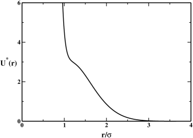
Figure 1: Interaction potential from eq. (1) with parameters $a=5,$ $r_{0}/\sigma=0.7$ and $c=1$, in reduced units.

Figure 2: Interaction potential from eq. (2) with parameter $\sigma_{1}/\sigma=1.75$ in reduced units.

The second model we study here is a system of $N$ particles of diameter $\sigma,$ inside a cubic box whose volume is $V,$ resulting in a density number $\rho=N/V$ but interacting with a discontinuous shoulder potential given by

$$U^{*}(r)=\cases{\infty&$r<\sigma$\cr 1&$\sigma_{1}>r>\sigma$\cr 0&$r>\sigma_{1}$}\;,$$ (2)

where $U^{*}(r)=U(r)/\epsilon.$ This potential has two natural length scales: the hard core distance, $\sigma,$ and the outer core, $\sigma_{1}$. Here we analyze the case $\sigma_{1}/\sigma=1.75$ illustrated in Fig. 2. Here we use dimensionless pressure, $P^{*},$ temperature, $T^{*},$ and density, $\rho^{*},$ that are given in units of $\sigma^{3}/\epsilon$, $k_{B}/\epsilon,$ and $\sigma^{3},$ respectively and $k_{B}$ stands for the Boltzmann constant.

3 Details of simulations

For the continuous shoulder potential we performed molecular dynamics simulations. Details of the simulation can be found in ref Ol06a .

Figure 3: Pressure-temperature phase-diagram obtained for the continuous shoulder potential. From bottom to top $\rho^{*}=$ 0.100, 0.103, 0.105, 0.107 0.110, 0.113, 0.115, 0.117, 0.120, 0.123, 0.125, 0.127, 0.130, 0.132, 0.134, 0.136, 0.138, 0.140, 0.142, and 0.144 are shown. The solid line illustrates the TMD and the dashed lines show the boundary of the diffusivity extrema.

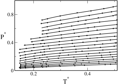
Figure 4: Pressure-temperature phase-diagram for the discontinuous shoulder potential. From bottom to top $\rho^{*}=$ 0.08, 0.09, 0.10, 0.11, 0.12, 0.13, 0.14, 0.15, 0.16, 0.17, 0.18, 0.19, 0.20, 0.21, 0.22, 0.23, 0.24, 0.25, and 0.26 are shown.

Figure (3) shows the P-T phase-diagram we have obtained in a previous publication Ol06a . The isochores have minima that define the temperature of maximum density. The TMD line encloses the region of density (and entropy) anomaly. We also have studied the mobility associated with the potential described in Eq. (1) Ol06a . The diffusion was also calculated using the the mean-square displacement averaged over different initial times. The behavior of $D$ as a function of $\rho^{*}$ goes as follows. At low temperatures, the behavior is similar to the behavior found in SPC/E supercooled water Ne01 . The diffusivity increases as the density is lowered, reaches a maximum at $\rho_{D{\rm max}}$ (and $P_{D{\rm max}}$) and decreases until it reaches a minimum at $\rho_{D{\rm min}}$ (and $P_{D{\rm min}}$). The region in the P-T plane where there is an anomalous behavior in the diffusion is bounded by $(T_{D{\rm min}},$ $P_{D{\rm min}})$ and $(T_{D{\rm max}},$ $P_{D{\rm max}})$ and their location is shown in Fig.  (3). The region of diffusion anomalies $(T_{D{\rm max}}$, $P_{D{\rm max}})$ and $(T_{D{\rm min}},$ $P_{D{\rm min}})$ lies outside the region of density anomalies like in SPC/E water Ne01 .

In order to simulate the discrete potential showed in Fig. (2) we used the collision driven molecular dynamics techniques Al59 . 500 particles were put into a simulation box with periodic boundary conditions and the rescaling velocities scheme was used for every 1000 collisions until equilibration time to achieve the desired temperature. After thermalization particles were allowed to move under microcanonical ensemble. In the collision driven molecular dynamics simulation, kinetic energy has to be rigorously conserved. Hence, no special mechanism is necessary in order to simulate a desired temperature and the NVE ensemble becomes the natural choice. The equilibration and production times in reduced units were 350 and 650 respectively. Figure (4) shows the P-T phase-diagram for the discontinuous shoulder potential. The isochores for different temperature and pressures show no minima so no density anomaly is present.

4 Excess entropy and anomalies

Why the discontinuous shoulder potential has no water-like anomalies and its continuous counterpart has all of them? We can gain some understanding about that by analyzing the density dependence of the excess entropy. Errington et al. have shown that the density anomaly is given by the condition $\Sigma_{\mathrm{ex}}=\left(\partial s_{\mathrm{ex}}/\partial\ln\rho\right)_{T}>1$ Er06 . Here $s_{\mathrm{ex}}$ is the excess entropy and is approximated by its two-body contribution,

$$s_{2}=-2\pi\rho\int\left[g(r)\ln g(r)-g(r)+1\right]r^{2}dr\;.$$

The radial distribution function, $g(r)$, is proportional to the probability to find a particle at a distance $r$ to another particle placed at the origin. Errington et al. Er06 have also suggested that the diffusion anomaly can be predicted by using the empirical Rosenfeld’s parameterization Ro99 . They found the condition $\Sigma_{2}>0.42$ for a diffusion anomalous behaviour. They also claim that $\Sigma_{2}>0$ is a good estimative for determining the region where structural anomaly occurs Er06 .

In order to understand the differences between the continuous and the discontinuous shoulder potentials we test the excess entropy criteria described above in both potentials. The radial distribution functions for different temperatures and densities for both potentials were then obtained by the molecular dynamic simulation method described in Sec. 3.

Figure (5) illustrates the two-body contribution of excess entropy for the continuous potential given by Eq. (1). $s_{2}$ is negative and its slope changes from positive to negative what indicates the presence of structural anomaly. Figure (6) shows the behavior of $\Sigma_{2}$ with density for a fixed temperature for the continuous model. The horizontal lines at $\Sigma_{2}^{t}=$ 0, 0.42, and 1 indicate the threshold beyond which there are structural, diffusion, and density anomalies respectively. In accordance with Fig. (3) the density anomalous region shown in Fig. (6) occurs in an interval of density smaller than the interval where the diffusion is anomalous. The two-body excess entropy also show the presence of structural anomaly what corroborates results of simulations of structural parameters Ol06b .

Figure (7) illustrates the two-body excess entropy of the discontinuous potential given by Eq. (2). $s_{2}$ is negative but its slope is for almost all temperatures and densities negative. The filled circles show the region where the system crystallization occur. Figure (8) shows the behavior of $\Sigma_{2}$ with density for fixed temperatures for the discontinuous model. The line $\Sigma_{2}^{t}=1$ is never crossed so no density anomaly should be expected what is in good agreement with the Fig. (4). The line $\Sigma_{2}^{t}=0.42$ is also never crossed what indicates that diffusion anomaly is not expected in the discontinuous model. This is also in agreement with results for similar step potentials where no diffusion anomaly is found for large steps Ne06 . The line $\Sigma_{2}=0$ is crossed for temperatures $T^{*}=$ 0.17 and 0.2 what would suggest the presence of structural anomaly. However this has to be taken with a grain of salt since Errington et al. Er06 demonstrated that $s_{2}$ overestimates the region of anomalies. In this sense, a detailed study of translational and orientational order parameters Ol06b is necessary prior to any affirmative on the presence of structural anomaly for this discontinuous shoulder.

Even thought the excess entropy criteria is quite useful for predicting if the anomalies would be present for a certain potential it does not provide an easy and intuitive method for understanding why the continuous shoulder has anomalies and the discontinuous one does not have. In principle, both potential exhibit similar characteristics. Both potentials have two repulsive scales and consequently the radial distribution function in both cases has two peaks, one close to the hard core and another close to the distance $r=\sigma_{1}$ as illustrated in Fig. (9) for the continuous potential and in Fig. (10) for the discontinuous potential. A closer look at the radial distribution reveals an important difference between the two cases. For the continuous potential for densities and temperatures in the region where anomalies occur $g(r)$ grows with density for $r/\sigma\approx 1$ and decreases with increasing density for $r\approx\sigma_{1}$ [see Fig. (9) for example]. For the discontinuous potential the $g(r)$ increases with density both at the hard core and at $r=\sigma_{1}$ for any temperature and density [see Fig. (10) for example]. Notice that the radial distribution function in both cases has significative changes with the change in density at the two natural scales.

Finally we propose that a two scale potential has anomalies for some temperature and densities if $\partial g(r)/\partial\rho>0$ for $r\approx\sigma$ and $\partial g(r)/\partial\rho<0$ for $r\approx\sigma_{1}$. If this requirements would not be fulfill for any temperature and density no anomaly would be present. This proposition is based in the physical picture that within the anomalous region for a fixed temperature an increase is density implies an increase in the number of particles close to the hard core. This particles move from the distance $\sigma_{1}$ to $\sigma$. For a discontinuous potential this requires an activation energy of $U=\epsilon$ while for the continuous case it can be done continuously. As it was shown by Netz et al. Ne06 for the steps potential, anomalies would only be observed if the discontinuity in $U^{*}$ would be below a certain threshold.

Now we shall test if this simple hypothesis is in agreement with Errington et al. criteria. First we compute $\Sigma_{2}$ as

$$\Sigma_{2} = \left(\frac{\partial s_{\mathrm{{ex}}}}{\partial\ln\rho}\right)_{T}$$

$$= s_{2}-2\pi\rho^{2}\int\ln g(r)\frac{\partial g(r)}{\partial\rho}r^{2}dr$$

In this expression, the first term is always negative for all two scale potentials. The integral in the second term, as we have observed above, is dominated by the the values at the two scales, $\sigma$ and $\sigma_{1}$.

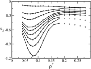
Figure 5: Pair contribution of excess entropy, $s_{2}$, against density for $T^{*}=$ 0.25, 0.30, 0.35, 0.40, 0.45, 0.50, 0.70, 1.00, and 3.00 from bottom to top for the continuous shoulder model (Fig.(1) . Circles are simulated data and lines are fifth order polynomial fit from data.

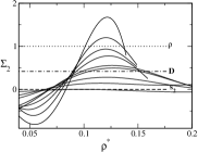
Figure 6: $\Sigma_{2}=\left(\partial s_{2}/\partial\ln\rho\right)_{T}$ versus density. Following the isochore $\rho^{*}=0.10$, from top to bottom, temperatures $T^{*}=$ 0.25, 0.30, 0.35, 0.40, 0.45, 0.50, 0.70, 1.00, and 3.00 are shown for the continuous shoulder potential.

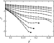
Figure 7: Pair contribution of excess entropy, $s_{2},$ against density for $T^{*}=$ 0.15, 0.17, 0.20, 0.23, 0.25, 0.30, 0.35, 0.40, 0.45, and 0.50 from bottom to top for the discontinuous shoulder model (Fig.(2). Open circles are simulated data and lines are fifth order polynomial fit from data. Solid circles show the limit of crystalization.

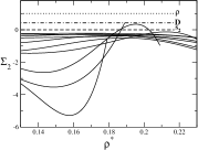
Figure 8: $\Sigma_{2}=\left(\partial s_{2}/\partial\ln\rho\right)_{T}$ versus density for the discontinuous shoulder potential. Following the isochore $\rho^{*}=0.13,$ from bottom to top, $T^{*}=$ 0.15, 0.17, 0.20, 0.23, 0.25, 0.30, 0.35, 0.40, 0.45, and 0.5 are shown.

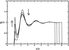
Figure 9: Radial distribution function for the potential given by Eq. (1) for $T^{*}=0.25$ and densities $\rho^{*}=$ 0.12, 0.14, 0.16, and 0.18. Arrows indicate the direction of increasing $\rho^{*}.$

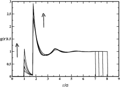
Figure 10: Radial distribution function for the potential given by Eq. (2) for $T^{*}=0.25$ and densities $\rho^{*}=$ 0.12, 0.14, 0.16, and 0.18. Arrows indicate the direction of increasing $\rho^{*}.$

For the continuous potential in the region where the anomaly is present $\ln g(r\approx\sigma)<1$ while $\ln g(r\approx\sigma_{1})>1$. Also $\partial g(\sigma)/\partial\rho>0$ while $\partial g(\sigma_{1})/\partial\rho<0$. Consequently the second term in Eq. (4) is positive. This allows for a zero or positive values of $\Sigma_{2}$ for appropriated densities and temperatures. Therefore our criteria is in accord with Errington et al. criteria.

In resume, in this paper we have calculated the excess entropy and its derivative for both continuous and discontinuous shoulder potential. For the continuous case, using the Errington et al. criteria indicates that this potential has density, diffusion and structural anomalies as we have shown in previous publications. For the discontinuous potential the criteria indicates that no thermodynamic and dynamic anomalies are present and its not conclusive for structural anomalies. Direct calculations of the P-T temperature phase-diagram confirms the excess of entropy prediction. On basis of these results we propose a criteria for predicting if a two scale potential has or not anomalies. Our criteria provides a simple picture for the anomalies not being observed in the discontinuous shoulder potential.

We thank for financial support of the Brazilian science agencies CNPq, CAPES, and FINEP. One of the authors (A.B.O.) is indebted to Jeetain Mittal of NIH for his valuable discussions on collision driven molecular dynamics techniques.

References

- (1) R. Waler, Essays of natural experiments (Johnson Reprint, New York, 1964)
- (2) M. Chaplin, Sixty-three anomalies of water, http: (2006)
- (3) C.A. Angell, E.D. Finch, P. Bach, J. Chem. Phys. 65, 3065 (1976)
- (4) P.A. Netz, F.W. Starr, H.E. Stanley, M.C. Barbosa, J. Chem. Phys. 115, 344 (2001)
- (5) J.R. Errington, P.D. Debenedetti, Nature (London) 409, 318 (2001)
- (6) J. Mittal, J.R. Errington, T.M. Truskett, J. Phys. Chem. B 110, 18147 (2006)
- (7) F.H. Stillinger, A. Rahman, J. Chem. Phys. 60, 1545 (1974)
- (8) H.J.C. Berendsen, J.R. Grigera, T.P. Straatsma, J. Chem. Phys. 91, 6269 (1987)
- (9) M.W. Mohoney, W.L. Jorgensen, J. Chem. Phys. 112, 8910 (2000)
- (10) M.R. Sdr-Lahijany, A. Scala, S.V. Buldyrev, H.E. Stanley, Phys. Rev. Lett. 81, 4895 (1998)
- (11) G. Franzese, G. Malescio, A. Skibinsky, S.V. Buldyrev, H.E. Stanley, Nature (London) 409, 692 (2001)
- (12) A. Balladares, M.C. Barbosa, J. Phys.: Cond. Matter 16, 8811 (2004)
- (13) A.B. de Oliveira, M.C. Barbosa, J. Phys.: Cond. Matter 17, 399 (2005)
- (14) V.B. Henriques, M.C. Barbosa, Phys. Rev. E 71, 031504 (2005)
- (15) V.B. Henriques, N. Guissoni, M.A. Barbosa, M. Thielo, M.C. Barbosa, Mol. Phys. 103, 3001 (2005)
- (16) E.A. Jagla, Phys. Rev. E 58, 1478 (1998)
- (17) H.M. Gibson, N.B. Wilding, Phys. Rev. E 73, 061507 (2006)
- (18) P. Camp, Phys. Rev. E 68, 061506 (2003)
- (19) A.B. de Oliveira, P.A. Netz, T. Colla, M.C. Barbosa, J. Chem. Phys. 124, 084505 (2006)
- (20) A.B. de Oliveira, P.A. Netz, T. Colla, M.C. Barbosa, J. Chem. Phys. 125, 124503 (2006)
- (21) R. Sharma, S.N. Chakraborty, C. Chakravarty, J. Chem. Phys. 125, 204501 (2006)
- (22) J.R. Errington, T.M. Truskett, J. Mittal, J. Chem. Phys. 125, 244502 (2006)
- (23) B.J. Alder, T.E. Wainwright, J. Chem. Phys. 31, 459 (1959)
- (24) Y. Rosenfeld, J. Phys.: Condens. Matter 11, 5415 (1999)
- (25) P.A. Netz, S. Buldyrev, M.C. Barbosa, H.E. Stanley, Physical Review E 73, 061504 (2006)