American Options under Proportional Transaction Costs: Pricing, Hedging and Stopping Algorithms for Long and Short Positions

Abstract

American options are studied in a general discrete market in the presence of proportional transaction costs, modelled as bid-ask spreads. Pricing algorithms and constructions of hedging strategies, stopping times and martingale representations are presented for short (seller’s) and long (buyer’s) positions in an American option with an arbitrary payoff. This general approach extends the special cases considered in the literature concerned primarily with computing the prices of American puts under transaction costs by relaxing any restrictions on the form of the payoff, the magnitude of the transaction costs or the discrete market model itself. The largely unexplored case of pricing, hedging and stopping for the American option buyer under transaction costs is also covered. The pricing algorithms are computationally efficient, growing only polynomially with the number of time steps in a recombinant tree model. The stopping times realising the ask (seller’s) and bid (buyer’s) option prices can differ from one another. The former is generally a so-called mixed (randomised) stopping time, whereas the latter is always a pure (ordinary) stopping time.

1 Introduction

In this paper we study the seller’s and buyer’s positions in American options when trading in the underlying asset is subject to proportional transaction costs. The results apply to options with arbitrary payoffs in any discrete market model and proportional transaction costs of any magnitude. We are concerned with computing the seller’s price of an American option, also known as the upper hedging price or the ask price, as well as the buyer’s price, often referred to as the lower hedging price or the bid price. Apart from pricing, we construct optimal strategies superhedging the positions of the option seller and buyer, together with the respective stopping times realising the option prices, generally a mixed (randomised) stopping time for the seller and a pure (ordinary) stopping time for the buyer. We also consider martingale representations for the ask and bid option prices.

The first to examine American options under proportional transaction costs in a similar setting and level of generality as in the present paper were Chalasani and Jha [CJ01]. They established martingale representations for options with cash settlement, subject to the simplifying assumption that transaction costs apply at any time, except at any particular stopping time chosen by the buyer to exercise the option. An important feature that emerged in Chalasani and Jha’s representation for the option seller’s price was the role played by mixed stopping times in place of pure stopping times. Chalasani and Jha pointed out the non-trivial nature of computing the option prices in their representations and the need to develop algorithms to evaluate these prices. Our pricing algorithms solve this problem. Moreover, we put forward algorithms for constructing the corresponding hedging strategies, stopping times, and approximate martingales.

Bouchard and Temam [BT05] established a dual representation for the set of initial endowments allowing to superhedge the seller’s position in an American option in a discrete time market model with proportional transaction costs in the setting of Kabanov, Rásonyi and Stricker [KRS03], and Schachermayer [Sch04]. In particular, they reproduced Chalasani and Jha’s [CJ01] martingale representation of the seller’s price. However, note that Bouchard and Temam [BT05] follow a different convention than Chalasani and Jha [CJ01] in that they rebalance the portfolios in a hedging strategy before rather than after it becomes known whether or not the American option is to be exercised.

Papers concerned with various special cases involving the hedging prices of American options under proportional transaction costs include Kociński [Koc99], [Koc01], who studied sufficient conditions for the existence of perfectly replicating strategies for American options, Perrakis and Lefoll [PL00], [PL04], who investigated American calls and puts in the binomial model, and Tokarz and Zastawniak [TZ06], who worked with general American payoffs in the binomial model under small proportional transaction costs.

Another group of papers, using preference-based or risk minimisation approaches rather than superhedging for American options under proportional transaction costs, includes Davis and Zariphopoulou [DZ95], Mercurio and Vorst [MV97], Constantinides and Zariphopoulou [CZ01], and Constantinides and Perrakis [CP04]. The work by Levental and Skorohod [LS97], and Jakubenas, Levental and Ryznar [JLR03] shows that superhedging in continuous time leads to unrealistic results for American options under proportional transaction costs, thus providing motivation for exploring discrete time approaches.

The present paper complements and extends the results obtained by Chalasani and Jha [CJ01] and Bouchard and Temam [BT05] by providing pricing, hedging, stopping and approximate martingale algorithms for arbitrary American options under proportional transaction costs in a general discrete setting. It also extends the work on hedging prices by several of the authors listed above, removing any restrictions imposed in the various special cases that have been considered in the literature. As a by-product, we establish the same martingale representations for American option prices under transaction costs as in [CJ01] or [BT05] by a very different method based on an explicit construction of the stopping times and approximate martingales representing the ask and bid option prices. The construction provides a geometric insight into the origin of mixed stopping times in the seller’s case. Some of the results presented here have first been established in [Rou06].

In the well-known case without transaction costs a stopping time that is best for the option holder (the buyer) also happens to be the worst one for the option writer (the seller). Similarly, a strategy hedging a shorted option is essentially the opposite to a strategy hedging a long position in the option. This kind of symmetry between the option seller and buyer breaks down in the presence of transaction costs. Hedging against a stopping time that is optimal for the buyer will generally no longer protect the seller against all other possible exercise times. To hedge against all pure stopping times, the seller must in effect be protected against a certain mixed stopping time. Moreover, under transaction costs a simple relationship generally no longer exists between strategies hedging long and short positions in the option. These points are illustrated by the ‘clinical’ example in Section 4.

In the presence of transaction costs hedging against all stopping times can cost more than against the buyer’s optimal stopping time. If the seller knew with certainty that the option will be exercised at the buyer’s optimal stopping time, then it would only be necessary to hedge against this single stopping time, making the seller’s hedging strategy less expensive. However the option would then no longer be of American type. This situation is reminiscent of a Nash equilibrium.

A deeper mathematical reason behind the apparent lack of symmetry between buyer and seller under transaction costs is that pricing for the seller as defined by (3.2) is a convex optimisation problem, whereas the buyer’s pricing problem (3.4) is not of this kind, in general. This is reflected in the pricing, hedging and stopping algorithms for the option seller presented in this paper, which operate within the space of convex functions (and thus have convex dual counterparts involving concave functions), whereas the corresponding buyer’s algorithms no longer act on convex functions alone.

Computing the seller’s and buyer’s prices of an American option directly from the definitions (3.2) and (3.4) amounts to solving large optimisation problems over the corresponding set of superhedging strategies. Both these optimisation problems grow exponentially with the number of time steps, as observed (for European options) by Rutkowski [Rut98] and Chen, Sheu and Palmer [CPS07]. In Algorithm 3.1 (and the equivalent convex dual Algorithm 3.2) for the seller’s price and in Algorithm 3.5 for the buyer’s price we present computationally efficient dynamic programming type iterative procedures, which grow only polynomially with the number of time steps in a recombinant tree model. It is shown in Remark 3.2 that Algorithm 3.2 can be regarded as an extension of the familiar Snell envelope construction to the case with transaction costs.

Numerical examples are provided to demonstrate the flexibility and efficiency of the pricing algorithms in a realistic market model approximation. The algorithms presented in this paper apply to options with arbitrary payoffs in general discrete market models, including incomplete ones, with arbitrary proportional transaction costs. The efficiency of the pricing algorithms (due to their polynomial growth) makes it possible to cover a considerably larger range of time steps and parameter values than in the latest numerical work by Perrakis and Lefoll [PL04], and to extend the numerical computations beyond the binomial tree model as well as beyond puts or calls to include long and short positions in option baskets (which are, of course, not equivalent to a combination of puts and calls in the presence of transaction costs).

The contents of this paper are organised as follows. In Section 2 we fix the notation, specify the market model with transaction costs, and present the necessary information on mixed stopping times, approximate martingales and the families of functions to be used throughout the paper. Section 3 is the main part of the paper. Following some definitions, pricing, hedging, stopping and approximate martingale algorithms are presented here for both the seller and the buyer of an American option in the presence of proportional transaction costs, along with theorems proving the correctness of these algorithms. A simple illustrative example, which can be followed by hand, showing the algorithms in action can be found in Section 4. In Section 5 we produce a number of more realistic numerical examples. Finally, Section 6 serves as an appendix containing some technical results.

2 Preliminaries

2.1 Market Model

Consider a finite probability space $\Omega$ with the field $\mathcal{F}=2^{\Omega}$ of all subsets of $\Omega$, a probability measure $Q$ on $\mathcal{F}$ such that $Q\{\omega\}>0$ for each $\omega\in\Omega$, and a filtration $\left\{\emptyset,\Omega\right\}=\mathcal{F}_{0}\subset\mathcal{F}_{1}\subset\cdots\subset\mathcal{F}_{T}=\mathcal{F}$, the time horizon $T$ being a positive integer. For each $t=0,1,\ldots,T$ we denote by $\Omega_{t}$ the set of atoms of $\mathcal{F}_{t}$, and identify any $\mathcal{F}_{t}$-measurable random variable $X$ with a function defined on $\Omega_{t}$. We shall write $X^{\mu}$ to indicate the value of $X$ at $\mu\in\Omega_{t}$. Any probability measure $P$ on $\mathcal{F}$ can be identified with the family of probability measures $P_{t}$ on $\mathcal{F}_{t}$ such that $P_{t}(\mu)=P(\mu)$ for each $\mu\in\Omega_{t}$ and $t=0,1,\ldots,T$.

The filtration can be represented as a tree, the atoms of $\mathcal{F}_{t}$ corresponding to the nodes of the tree at time $t$. We shall say that $\nu\in\Omega_{t+1}$ is a successor node of $\mu\in\Omega_{t}$ if $\nu\subset\mu$, this relationship corresponding to the branches of the tree. The set of successor nodes of $\mu\in\Omega_{t}$ will be denoted by

$$\operatorname*{succ}\mu=\{\nu\in\Omega_{t+1}\,|\,\nu\subset\mu\}.$$

The market model consists of a risk-free bond and a risky stock. There are proportional transaction costs on stock trades expressed as bid-ask spreads, as in Jouini and Kallal [JK95]. Shares can be bought at the ask price $S_{t}^{\mathrm{a}}$ or sold at the bid price $S_{t}^{\mathrm{b}}$, where $S_{t}^{\mathrm{a}}\geq S_{t}^{\mathrm{b}}>0$ for each $t=0,1,\ldots,T$, the processes $S^{\mathrm{a}}$ and $S^{\mathrm{b}}$ being adapted to the filtration. Without loss of generality, we can assume that all prices are discounted, the bond price being $1$ for each $t=0,1,\ldots,T$, so that a position in bonds can be identified with cash holdings.

A portfolio $\left(\gamma,\delta\right)$ of cash (or bonds) and stock can be liquidated at time $t$ by selling stock for $S_{t}^{\mathrm{b}}$ per share to close a long position $\delta\geq 0$ or buying stock for $S_{t}^{\mathrm{a}}$ per share to close a short position $\delta<0$. The liquidation value of the portfolio will be

$$\vartheta_{t}(\gamma,\delta)=\gamma+S_{t}^{\mathrm{b}}\delta^{+}-S_{t}^{\mathrm{a}}\delta^{-}.$$

The cost of setting up a portfolio $(\gamma,\delta)$ is

$$-\vartheta_{t}(-\gamma,-\delta)=\gamma-S_{t}^{\mathrm{b}}\delta^{-}+S_{t}^{\mathrm{a}}\delta^{+}.$$

A self-financing strategy is a predictable process $(\alpha_{t},\beta_{t})$ representing positions in cash (or bonds) and stock at $t=0,\ldots,T$ such that

$$\vartheta_{t}(\alpha_{t}-\alpha_{t+1},\beta_{t}-\beta_{t+1})\geq 0$$ (2.1)

for each $t=0,\ldots,T-1$. The set of all self-financing strategies will be denoted by $\Phi$. An arbitrage opportunity is a self-financing strategy $\left(\alpha,\beta\right)\in\Phi$ such that

$$-\vartheta_{0}(-\alpha_{0},-\beta_{0})\leq 0,\quad\vartheta_{T}(\alpha_{T},\beta_{T})\geq 0,\quad Q\left\{\vartheta_{T}(\alpha_{T},\beta_{T})>0\right\}>0.$$

It was established by Jouini and Kallal [JK95] that the lack of arbitrage in the model with proportional transaction costs is equivalent to the existence of a probability measure $P$ on $\Omega$ equivalent to $Q$ and a martingale $S$ under $P$ such that $S_{t}^{\mathrm{b}}\leq S_{t}\leq S_{t}^{\mathrm{a}}$ for each $t=0,1,\ldots,T$. This result also follows from Kabanov and Stricker [KS01], Ortu [Ort01], Kabanov, Rásonyi and Stricker [KRS02], [KRS03], Tokarz [Tok04], and Schachermayer [Sch04].

2.2 Mixed Stopping Times

A stopping time $\tau$ is a random variable such that $\left\{\tau=t\right\}\in\mathcal{F}_{t}$ for each $t=0,1,\ldots,T$. The set of stopping times $\tau$ with values in $\left\{0,1,\ldots,T\right\}$ will be denoted by $\mathcal{T}$. To distinguish them from mixed stopping times, defined below, we shall sometimes refer to such $\tau$’s as pure stopping times.

A mixed stopping time (also called a randomised stopping time as in, for example, Chow, Robins and Siegmund [CRS71], Baxter and Chacon [BC77], or Chalasani and Jha [CJ01]) is defined as a non-negative adapted process $\chi$ such that

$$\sum_{t=0}^{T}\chi_{t}=1.$$

The set of all mixed stopping times will be denoted by $\mathcal{X}$. We have $\mathcal{T}\subset\mathcal{X}$ in the sense that each pure stopping time $\tau$ can be identified with a mixed stopping time $\chi^{\tau}$ such that for any $t=0,1,\ldots,T$

$$\chi_{t}^{\tau}=1_{\left\{\tau=t\right\}}.$$

For any adapted process $Z$ and any mixed stopping time $\chi$ the time-$\chi$ value of $Z$ is defined as

$$Z_{\chi}=\sum_{t=0}^{T}\chi_{t}Z_{t}.$$

If $\tau$ is a pure stopping time, then $Z_{\chi^{\tau}}$ is the familiar random variable

$$Z_{\chi^{\tau}}=\sum_{t=0}^{T}1_{\left\{\tau=t\right\}}Z_{t}=Z_{\tau}.$$

For any mixed stopping time $\chi\in\mathcal{X}$ and any adapted process $Z$ we define processes $\chi^{\ast}$ and $Z^{\chi^{\ast}}$ such that for each $t=0,1,\ldots,T$

$$\chi_{t}^{\ast}=\sum_{s=t}^{T}\chi_{s},\quad Z_{t}^{\chi^{\ast}}=\sum_{s=t}^{T}\chi_{s}Z_{s}.$$ (2.2)

In addition, it will prove convenient to put

$$\chi_{T+1}^{\ast}=0,\quad Z_{T+1}^{\chi^{\ast}}=0.$$ (2.3)

2.3 Approximate Martingales

As observed in Section 2.1, a market model with proportional transaction costs does not admit arbitrage if and only if there exists a pair $(P,S)$ consisting of a probability measure $P$ on $\Omega$ equivalent to $Q$ and a martingale $S$ under $P$ such that for each $t=0,1,\ldots,T$

$$S_{t}^{\mathrm{b}}\leq S_{t}\leq S_{t}^{\mathrm{a}}.$$

The family of such pairs $(P,S)$ will be denoted by $\mathcal{P}$. If the condition that $P$ should be equivalent to $Q$ is relaxed, then the corresponding family of pairs $(P,S)$ is to be denoted by $\mathcal{\bar{P}}$. The families $\mathcal{P}$ and $\mathcal{\bar{P}}$ can be used to represent the prices of European options under proportional transaction costs, see Jouini and Kallal [JK95]. To represent the prices of American options we need certain larger families than $\mathcal{P}$ or $\mathcal{\bar{P}}$.

For any mixed stopping time $\chi\in\mathcal{X}$ we denote by $\mathcal{P}(\chi)$ the family of pairs $(P,S)$ consisting of a probability measure $P$ on $\Omega$ equivalent to $Q$ and an adapted process $S$ such that for each $t=0,1,\ldots,T$

$$S_{t}^{\mathrm{b}}\leq S_{t}\leq S_{t}^{\mathrm{a}},$$ (2.4)

$$\chi_{t+1}^{\ast}S_{t}^{\mathrm{b}}\leq\mathbb{E}_{P}(S_{t+1}^{\chi^{\ast}}|\mathcal{F}_{t})\leq\chi_{t+1}^{\ast}S_{t}^{\mathrm{a}},$$ (2.5)

where $\mathbb{E}_{P}$ is the expectation under $P$. If the assumption that $P$ should be equivalent to $Q$ is relaxed, the corresponding family of pairs $(P,S)$ will be denoted by $\mathcal{\bar{P}}(\chi)$. A pair $(P,S)$ of this kind will be called an approximate martingale. For a pure stopping time $\tau\in\mathcal{T}$ we shall write $\mathcal{P}(\tau)$ and $\mathcal{\bar{P}}(\tau)$ instead of $\mathcal{P}(\chi^{\tau})$ and $\mathcal{\bar{P}}(\chi^{\tau})$. This notation and terminology resembles that in Chalasani and Jha [CJ01].

Form Proposition 6.1 we know that $\mathcal{P}\subset\mathcal{P}(\chi)$ and $\mathcal{\bar{P}}\subset\mathcal{\bar{P}}(\chi)$. It follows that the families $\mathcal{P}(\chi)$ and $\mathcal{\bar{P}}(\chi)$ are non-empty for any $\chi\in\mathcal{X}$ in an arbitrage-free market model, since $\mathcal{P}$ is non-empty and $\mathcal{P\subset\bar{P}}$.

2.4 Families of Polyhedral Functions

We denote by $\Theta$ the family of functions $f:\mathbb{R\rightarrow R\cup\{-\infty\}}$ such that $f\equiv-\infty$ or $f$ is an $\mathbb{R}$-valued polyhedral function (i.e. continuous piecewise linear function with a finite number of pieces).

For any $f,g$ in $\Theta$ the maximum and minimum of $f$ and $g$ also belong to $\Theta$. The epigraph of a function $f\in\Theta$ is given by

$$\operatorname*{epi}f=\{(x,y)\in\mathbb{R}^{2}\,|\,x\geq f(y)\}.$$

For any $a\geq b$ the function

$$h_{[b,a]}(y)=ay^{-}-by^{+}$$

belongs to $\Theta$. Observe that the self-financing condition (2.1) can be written as

$$(\alpha_{t}-\alpha_{t+1},\beta_{t}-\beta_{t+1})\in\operatorname*{epi}h_{[S_{t}^{\mathrm{b}},S_{t}^{\mathrm{a}}]}.$$

For each $f\in\Theta$ there is a unique function in $\Theta$, denoted by $\operatorname{gr}_{[b,a]}(f)$, such that

$$\operatorname*{epi}[\operatorname{gr}_{[b,a]}(f)]=\operatorname*{epi}h_{[b,a]}+\operatorname*{epi}f.$$

We shall call $\operatorname{gr}_{[b,a]}(f)$ the gradient restriction of $f$. This transformation is illustrated in Figure 2.1.

Figure 2.1: Gradient restriction of a function $f$ in $\Theta$

If $f\in\Theta$ is a function with finite values, then it has finite limits $f^{\prime}(+\infty)=\lim_{x\rightarrow+\infty}f^{\prime}(x)$ and $f^{\prime}(-\infty)=\lim_{x\rightarrow-\infty}f^{\prime}(x)$. If these limits satisfy the inequalities

$$b\leq-f^{\prime}(-\infty)\quad\text{and}\quad-f^{\prime}(+\infty)\leq a,$$ (2.6)

then $\operatorname{gr}_{[b,a]}(f)$ is also a function with finite values. The financial meaning of gradient restriction is that portfolios in the epigraph of $\operatorname{gr}_{[S_{t}^{\mathrm{b}},S_{t}^{\mathrm{a}}]}(f)$ are precisely those that can be rebalanced in a self-financing manner at time $t$ to yield a portfolio in the epigraph of $f$.

Computer implementation of the three operations in $\Theta$ mentioned above, namely the maximum, minimum, and gradient restriction, is straightforward. They will be used in pricing Algorithms 3.1 and 3.5, and in the numerical examples in Section 5.

We denote by $\Lambda$ the family of all convex functions in $\Theta$. It is closed under the maximum and gradient restriction operations, but not the minimum. For any $f\in\Lambda$ the convex dual is defined by

$$f^{\ast}(x)=\inf_{y\in\mathbb{R}}(f(y)+xy)$$

for each $x\in\mathbb{R}$. The infimum is attained whenever it is finite. Convex duality maps $\Lambda$ bijectively onto the family $\Gamma$ of concave functions $v:\mathbb{R\rightarrow R\cup\{-\infty\}}$ such that $v$ is polyhedral (continuous piecewise linear with a finite number of pieces) on its essential domain

$$\operatorname*{dom}v=\{x\in\mathbb{R}\,|\,v(x)>-\infty\}.$$

The inverse transform from $\Gamma$ to $\Lambda$ is given by

$$f(y)=\sup_{x\in\mathbb{R}}(f^{\ast}(x)-xy),$$ (2.7)

with the supremum attained whenever finite.

For any $v_{1},\ldots,v_{n}\in\Gamma$ we denote by $\operatorname*{cap}\{v_{1},\ldots,v_{n}\}$ the concave cap of $v_{1},\ldots,v_{n}\in\Gamma$, defined as the smallest concave function $v$ such that $v\geq v_{i}$ for each $i=1,\ldots,n$. It belongs to $\Gamma$ and for each $x\in\mathbb{R}$ can be represented as

$$\operatorname*{cap}\{v_{1},\ldots,v_{n}\}(x)=\max\sum_{i=1}^{n}\lambda_{i}v_{i}(x_{i}),$$ (2.8)

where the maximum is taken over all $\lambda_{1},\ldots,\lambda_{n}\geq 0$ and $x_{1},\ldots,x_{n}\in\mathbb{R}$ that satisfy

$$\sum_{i=1}^{n}\lambda_{i}=1,\quad\sum_{i=1}^{n}\lambda_{i}x_{i}=x,$$

and $x_{i}\in\operatorname*{dom}v_{i}$ for each $i=1,\ldots,n$ such that $\operatorname*{dom}v_{i}\neq\emptyset$, see Rockafellar [Roc97].

Under convex duality the convex cap in $\Gamma$ corresponds to the maximum in $\Lambda$,

$$\max\{f,g\}^{\ast}=\operatorname*{cap}\{f^{\ast},g^{\ast}\}$$

for any $f,g\in\Lambda$. The operation in $\Gamma$ corresponding to gradient restriction in $\Lambda$ will be called domain restriction. For each $v\in\Gamma$ and each $x\in\mathbb{R}$ it is defined by

$$\operatorname{dr}_{[b,a]}(v)(x)=\left\{\begin{array}[c]{ll}v(x)&\text{if }x\in[b,a],\\ -\infty&\text{if }x\notin[b,a].\end{array}\right.$$

For any $f\in\Lambda$ we have

$$\operatorname{gr}_{[b,a]}(f)^{\ast}=\operatorname{dr}_{[b,a]}(f^{\ast}).$$

If $f\in\Lambda$ has finite values, then

$$[-f^{\prime}(+\infty),-f^{\prime}(-\infty)]=\operatorname*{dom}f^{\ast},$$

and (2.6) can be written as

$$[b,a]\cap\operatorname*{dom}f^{\ast}\neq\emptyset.$$

This condition guarantees that $\operatorname{gr}_{[b,a]}(f)$ has finite values, or, equivalently, that $\operatorname{dr}_{[b,a]}(f^{\ast})$ has non-empty essential domain.

3 American Options under Proportional Transaction Costs

Let us take an adapted process $\left(\xi_{t},\zeta_{t}\right)$ with values in $\mathbb{R}^{2}\cup\{(-\infty,-\infty)\}$ defined for all $t=0,1,\ldots,T$ to be the payoff process of an American option. The seller of the option must deliver to the buyer a portfolio $(\xi_{\tau},\zeta_{\tau})$ of cash and stock at an exercise time $\tau\in\mathcal{T}$ chosen by the buyer.

The pair $(-\infty,-\infty)$ is included among the possible values of the payoff process to allow for the possibility that the option cannot be exercised at certain times or nodes of the tree. This ensures that the results of this paper are in fact valid not only for American options but also for European or Bermudan type derivatives.

The seller can hedge a short position in the option by a self-financing strategy $(\alpha,\beta)\in\Phi$ such that at each stopping time $\tau\in\mathcal{T}$ he or she will be left with a solvent portfolio $(\alpha_{\tau}-\xi_{\tau},\beta_{\tau}-\zeta_{\tau})$ once the payoff $(\xi_{\tau},\zeta_{\tau})$ has been delivered to the buyer, that is, a portfolio such that

$$\vartheta_{\tau}(\alpha_{\tau}-\xi_{\tau},\beta_{\tau}-\zeta_{\tau})\geq 0.$$ (3.1)

This is called a superhedging strategy for the seller. The cost of setting up such a strategy is $-\vartheta_{0}(-\alpha_{0},-\beta_{0})$, the lowest of which defines the the seller’s price (ask price, upper hedging price) of the option:

$$\pi^{\mathrm{a}}(\xi,\zeta)=\min\left\{-\vartheta_{0}(-\alpha_{0},-\beta_{0})|(\alpha,\beta)\in\Phi,\forall\tau\in\mathcal{T}:\vartheta_{\tau}(\alpha_{\tau}-\xi_{\tau},\beta_{\tau}-\zeta_{\tau})\geq 0\right\}.$$ (3.2)

On the other hand, the buyer can hedge a long position in the option by a self-financing strategy $(\alpha,\beta)\in\Phi$ such that there is a stopping time $\tau\in\mathcal{T}$ when he or she will be left with a solvent portfolio $(\alpha_{\tau}+\xi_{\tau},\beta_{\tau}+\zeta_{\tau})$ after exercising the option and receiving the payoff $(\xi_{\tau},\zeta_{\tau})$, that is, a portfolio such that

$$\vartheta_{\tau}(\alpha_{\tau}+\xi_{\tau},\beta_{\tau}+\zeta_{\tau})\geq 0.$$ (3.3)

This is called a superhedging strategy for the buyer. By setting up such a strategy the buyer can raise the amount $\vartheta_{0}(-\alpha_{0},-\beta_{0})$. The highest amount that can be raised in this way is called the buyer’s price (bid price, lower hedging price) of the option:

$$\pi^{\mathrm{b}}(\xi,\zeta)=\max\left\{\vartheta_{0}(-\alpha_{0},-\beta_{0})|(\alpha,\beta)\in\Phi,\exists\tau\in\mathcal{T}:\vartheta_{\tau}(\alpha_{\tau}+\xi_{\tau},\beta_{\tau}+\zeta_{\tau})\geq 0\right\}.$$ (3.4)

In a discrete arbitrage-free market model the minimum in (3.2) and the maximum in (3.4) are attained. A strategy $(\alpha,\beta)\in\Phi$ realising the minimum in (3.2) is referred to as the seller’s optimal strategy. A strategy $(\alpha,\beta)\in\Phi$ and a stopping time $\tau\in\mathcal{T}$ realising the maximum in (3.4) are called the buyer’s optimal strategy and buyer’s optimal stopping time.

The prices $\pi^{\mathrm{a}}(\xi,\zeta)$ and $\pi^{\mathrm{b}}(\xi,\zeta)$ provide the upper and lower bounds of the no-arbitrage interval of option prices. Moreover, these are liquidity prices at which the option can be bought or, respectively, sold on demand. Liquidity is important because options are often traded as part of a strategy to hedge other derivatives.

3.1 Seller’s Case

3.1.1 Seller’s Pricing Algorithms

Let $(\xi,\zeta)$ be the payoff process of an American option. For each $t=0,1,\ldots,T$  and each $y\in\mathbb{R}$ we put

$$u_{t}(y)=\xi_{t}+(y-\zeta_{t})^{-}S_{t}^{\mathrm{a}}-(y-\zeta_{t})^{+}S_{t}^{\mathrm{b}}.$$ (3.5)

This defines an adapted process $u_{t}\in\Lambda$. Observe that a strategy $(\alpha,\beta)\in\Phi$ satisfies sellers’s superhedging condition (3.1) for a stopping time $\tau\in\mathcal{T}$ if and only if $(\alpha_{\tau},\beta_{\tau})\in\operatorname*{epi}u_{\tau}$.

Algorithm 3.1

For $t=0,1,\ldots,T$ take $u_{t}\in\Lambda$ given by (3.5) and construct adapted processes $z_{t},v_{t},w_{t}\in\Lambda$ by backward induction as follows:

• For each $\mu\in\Omega_{T}$ put

  $$z_{T}^{\mu}=v_{T}^{\mu}=w_{T}^{\mu}=u_{T}^{\mu}.$$

• For each $t=1,\ldots,T$ and $\mu\in\Omega_{t-1}$ put

  $$z_{t-1}^{\mu}=\max\{v_{t-1}^{\mu},u_{t-1}^{\mu}\},$$ (3.6)

  where

  $$v_{t-1}^{\mu} =\operatorname{gr}_{[S_{t-1}^{\mathrm{b}\mu},S_{t-1}^{\mathrm{a}\mu}]}(w_{t-1}^{\mu}),$$ (3.7)

  $$w_{t-1}^{\mu} =\max\{z_{t}^{\nu}\,|\,\nu\in\operatorname*{succ}\mu\}.$$ (3.8)

The resulting function $z_{0}$ will be related in Lemma 3.1 to hedging the seller’s position in the American option $(\xi,\zeta)$. In Theorem 3.3 it will be shown that

$$\pi^{\mathrm{a}}(\xi,\zeta)=z_{0}(0).$$

This algorithm can also be stated in terms of the dual functions

$$Z_{t}=z_{t}^{\ast},\quad V_{t}=v_{t}^{\ast},\quad W_{t}=w_{t}^{\ast},\quad U_{t}=u_{t}^{\ast},$$

which belong to $\Gamma$. Observe that for each $t=0,1,\ldots,T$ and $x\in\mathbb{R}$

$$U_{t}(x)=\left\{\begin{array}[c]{ll}\xi_{t}+x\zeta_{t}&\text{if }x\in[S_{t}^{\mathrm{b}},S_{t}^{\mathrm{a}}],\\ -\infty&\text{if }x\notin[S_{t}^{\mathrm{b}},S_{t}^{\mathrm{a}}].\end{array}\right.$$ (3.9)

By the duality between $\Lambda$ and $\Gamma$, Algorithm 3.1 is equivalent to the following procedure.

Algorithm 3.2

For $t=0,1,\ldots,T$ take $U_{t}\in\Gamma$ given by (3.9) and construct adapted processes $Z_{t},V_{t},W_{t}\in\Gamma$ by backward induction as follows:

• For each $\mu\in\Omega_{T}$ put

  $$Z_{T}^{\mu}=V_{T}^{\mu}=W_{T}^{\mu}=U_{T}^{\mu}.$$

• For each $t=1,\ldots,T$ and $\mu\in\Omega_{t-1}$ put

  $$Z_{t-1}^{\mu}=\operatorname*{cap}\{V_{t-1}^{\mu},U_{t-1}^{\mu}\},$$ (3.10)

  where

  $$V_{t-1}^{\mu} =\operatorname{dr}_{[S_{t-1}^{\mathrm{b}\mu},S_{t-1}^{\mathrm{a}\mu}]}(W_{t-1}^{\mu}),$$ (3.11)

  $$W_{t-1}^{\mu} =\operatorname*{cap}\{Z_{t}^{\nu}\,|\,\nu\in\operatorname*{succ}\mu\}.$$ (3.12)

The function $Z_{0}$ will be related in Lemma 3.1 and Remark 3.4 to hedging the seller’s position in the American option $(\xi,\zeta)$. In Theorem 3.3 it will be shown that

$$\pi^{\mathrm{a}}(\xi,\zeta)=\max_{x\in\mathbb{R}}Z_{0}(x).$$

Remark 3.1

If the payoff is finite at some node $\mu\in\Omega_{t}$, that is, $(\xi_{t}^{\mu},\zeta_{t}^{\mu})\in\mathbb{R}^{2}$, then at each ancestor node $\nu\supset\mu$, where $\nu\in\Omega_{s}$ for some $s=0,1,\ldots,t$, the functions $W_{s}^{\nu},V_{s}^{\nu},Z_{s}^{\nu}$ constructed in Algorithm 3.2 have non-empty effective domains, and $w_{s}^{\nu},v_{s}^{\nu},z_{s}^{\nu}$ in Algorithm 3.1 take finite values. In particular, $z_{0}(0)$ and the maximum of $Z_{0}$ are then finite. Indeed, for any $(P,S)\in\mathcal{P}$ it can be shown by backward induction that the effective domains of $W_{s}^{\nu},V_{s}^{\nu},Z_{s}^{\nu}$ must contain $S_{s}^{\nu}$. In an arbitrage-free model $\mathcal{P}$ is non-empty, so that these effective domains must then also be non-empty.

Remark 3.2

Algorithm 3.2 can be viewed as a natural extension of the familiar Snell envelope construction. In the absence of transaction costs, when $S_{t}^{\mathrm{a}}=S_{t}^{\mathrm{b}}=S_{t}$ for all $t$, formula (3.9) simply defines the cash equivalent $U_{t}=\xi_{t}+\zeta_{t}S_{t}$ of the payoff process $(\xi_{t},\zeta_{t})$ for an American option with physical delivery, (3.11) and (3.12) give the continuation value $V_{t-1}=\mathbb{E}^{\ast}(Z_{t}|\mathcal{F}_{t-1})$, where $\mathbb{E}^{\ast}$ is the risk neutral expectation, and (3.10) becomes $Z_{t-1}=\max\{U_{t-1},V_{t-1}\}$.

The workings of Algorithms 3.1 and 3.2 will be illustrated in Example 4.1 and Figures 4.1 and 4.2 in a simple two-step binomial tree setting. The numerical results in Section 5 for an American put and a bull spread in the binomial and trinomial tree models are computed by implementing these algorithms. In a recombinant model these computations grow only polynomially with the number of time steps, resulting in efficient numerical work in a realistic setting.

3.1.2 Hedging Seller’s Position

The following algorithm makes it possible to construct a strategy superhedging a short (seller’s) position in an American option with payoff process $(\xi,\zeta)$ by starting from any portfolio in $\operatorname*{epi}z_{0}$.

Algorithm 3.3

Construct a strategy $(\alpha,\beta)\in\Phi$ by induction as follows:

• Take any $\mathcal{F}_{0}$-measurable portfolio $(\alpha_{0},\beta_{0})\in\operatorname*{epi}z_{0}$.

• Suppose that an $\mathcal{F}_{t}$-measurable portfolio $(\alpha_{t},\beta_{t})\in\operatorname*{epi}z_{t}$ has already been constructed for some $t=0,\ldots,T-1$. Since, by (3.6) and (3.7),

  $$\operatorname*{epi}z_{t}\subset\operatorname*{epi}v_{t}=\operatorname*{epi}h_{[S_{t}^{\mathrm{b}},S_{t}^{\mathrm{a}}]}+\operatorname*{epi}w_{t},$$

  there is an $\mathcal{F}_{t}$-measurable portfolio $(\alpha_{t+1},\beta_{t+1})\in\operatorname*{epi}w_{t}$ such that

  $$(\alpha_{t}-\alpha_{t+1},\beta_{t}-\beta_{t+1})\in\operatorname*{epi}h_{[S_{t}^{\mathrm{b}},S_{t}^{\mathrm{a}}]}.$$ (3.13)

  Because of (3.8) we have $(\alpha_{t+1},\beta_{t+1})\in\operatorname*{epi}z_{t+1}$, and since $(\alpha_{t+1},\beta_{t+1})$ is $\mathcal{F}_{t}$-measurable, it is also $\mathcal{F}_{t+1}$-measurable, completing the induction step.

Because (3.13) is equivalent to the self-financing condition (2.1), we know that $(\alpha,\beta)\in\Phi$. It will be shown in Lemma 3.1 that $(\alpha,\beta)$ is a superhedging strategy for the seller.

Remark 3.3

When implementing the iterative step in Algorithm 3.3, the portfolio $(\alpha_{t+1},\beta_{t+1})$ can be constructed from $(\alpha_{t},\beta_{t})$ as follows:

• If $\alpha_{t}\geq w_{t}(\beta_{t})$, then we put $(\alpha_{t+1},\beta_{t+1})=(\alpha_{t},\beta_{t})$. No rebalancing of the portfolio occurs in this case.

• If $\alpha_{t}<w_{t}(\beta_{t})$, then the equation

  $$\alpha_{t}+x^{-}S_{t}^{\mathrm{b}}-x^{+}S_{t}^{\mathrm{a}}=w_{t}(\beta_{t}+x)$$

  has a solution $x$, and we put

  $$(\alpha_{t+1},\beta_{t+1})=(\alpha_{t}+x^{-}S_{t}^{\mathrm{b}}-x^{+}S_{t}^{\mathrm{a}},\beta_{t}+x),$$

  which amounts to buying $x$ shares at the ask price $S_{t}^{\mathrm{a}}$ if $x>0$ or selling them at the bid price $S_{t}^{\mathrm{b}}$ if $x<0$. The equation for $x$ has a solution because $(\alpha_{t},\beta_{t})\in\operatorname*{epi}h_{[S_{t}^{\mathrm{b}},S_{t}^{\mathrm{a}}]}+\operatorname*{epi}w_{t}$.

The following result shows that $\operatorname*{epi}z_{0}$ can be characterised as the set of endowments $(\gamma,\delta)$ consisting of cash and stock that are sufficient to initiate a superhedging strategy for the seller.

Lemma 3.1

The following conditions are equivalent:

1. $(\gamma,\delta)\in\operatorname*{epi}z_{0}$.

2. There is a self-financing strategy $(\alpha,\beta)\in\Phi$ such that $(\alpha_{0},\beta_{0})=(\gamma,\delta)$ and $(\alpha_{t},\beta_{t})\in\operatorname*{epi}z_{t}$ for each $t=0,1,\ldots,T$.

3. There is a superhedging strategy $(\alpha,\beta)\in\Phi$ for the seller such that $(\alpha_{0},\beta_{0})=(\gamma,\delta)$.

Proof  $1)\Rightarrow 2)$. This follows directly from the construction in Algorithm 3.3.

$2)\Rightarrow 3)$. This is so because $\operatorname*{epi}z_{\tau}\subset\operatorname*{epi}u_{\tau}$ by (3.6) and the seller’s superhedging condition (3.1) can be written as $(\alpha_{\tau},\beta_{\tau})\in\operatorname*{epi}u_{\tau}$ for each $\tau\in\mathcal{T}$.

$3)\Rightarrow 1)$. If $(\alpha,\beta)\in\Phi$ is a strategy as in condition $3)$, we claim that $(\alpha_{t},\beta_{t})\in\operatorname*{epi}z_{t}$ for all $t=0,1,\ldots,T$. Condition $1)$ then follows immediately. We prove this claim by backward induction on $t$. Since $(\alpha_{T},\beta_{T})\in\operatorname*{epi}u_{T}=\operatorname*{epi}z_{T}$, the claim is valid for $t=T$. Suppose that the claim holds for some $t=1,\ldots,T$, that is, $(\alpha_{t},\beta_{t})\in\operatorname*{epi}z_{t}$. Since $(\alpha_{t},\beta_{t})$ is $\mathcal{F}_{t-1}$-measurable, it follows by (3.8) that $(\alpha_{t},\beta_{t})\in\operatorname*{epi}w_{t-1}$. Because the strategy is self-financing, we have $(\alpha_{t-1}-\alpha_{t},\beta_{t-1}-\beta_{t})\in\operatorname*{epi}h_{[S_{t-1}^{\mathrm{b}},S_{t-1}^{\mathrm{a}}]}$. As a result, $(\alpha_{t-1},\beta_{t-1})\in\operatorname*{epi}h_{[S_{t-1}^{\mathrm{b}},S_{t-1}^{\mathrm{a}}]}+\operatorname*{epi}w_{t-1}=\operatorname*{epi}v_{t-1}$ by (3.7). Moreover, since $(\alpha,\beta)$ is a superhedging strategy for the seller, $(\alpha_{t-1},\beta_{t-1})\in\operatorname*{epi}u_{t-1}$. We can conclude using (3.6) that $(\alpha_{t-1},\beta_{t-1})\in\operatorname*{epi}v_{t-1}\cap\operatorname*{epi}u_{t-1}=\operatorname*{epi}z_{t-1}$. The claim has been verified.  

Remark 3.4

By duality, since $z_{t}(y)=\sup_{x\in\mathbb{R}}(Z_{t}(x)-xy)$, conditions $1)$ and $2)$ in Lemma 3.1 can be written, equivalently, as follows:

1. $\gamma+x\delta\geq Z_{0}(x)$ for each $x\in\mathbb{R}$.

2. There is a self-financing strategy $(\alpha,\beta)\in\Phi$ such that $(\alpha_{0},\beta_{0})=(\gamma,\delta)$ and $\alpha_{t}+x\beta_{t}\geq Z_{t}(x)$ for each $x\in\mathbb{R}$ and each $t=0,1,\ldots,T$.

3.1.3 Seller’s Stopping Time and Approximate Martingale

Our aim in this section is to construct a mixed stopping time $\hat{\chi}\in\mathcal{X}$ together with an approximate martingale $(\hat{P},\hat{S})\in\mathcal{\bar{P}}(\hat{\chi})$ so that the ask price of an American option with payoff process $(\xi,\zeta)$ can be expressed as

$$\pi^{\mathrm{a}}(\xi,\zeta)=\mathbb{E}_{\hat{P}}((\xi+\hat{S}\zeta)_{\hat{\chi}}).$$ (3.14)

At the same time, we shall also construct certain auxiliary adapted processes $\hat{\lambda},\hat{p},\hat{X},\hat{Y},\hat{Z},\hat{U},\hat{V}$.

Algorithm 3.4

Construct a mixed stopping time $\hat{\chi}\in\mathcal{X}$, a probability measure $\hat{P}$ and adapted processes $\hat{\lambda},\hat{p},\hat{S},\hat{X},\hat{Y},\hat{Z},\hat{U},\hat{V}$ by induction as follows:

• For $t=0$ there is a $\hat{Y}_{0}\in[S_{0}^{\mathrm{b}},S_{0}^{\mathrm{a}}]$ such that

  $$Z_{0}(\hat{Y}_{0})=\max_{x\in\mathbb{R}}Z_{0}(x).$$

  By (2.8), since $Z_{0}=\operatorname*{cap}\{V_{0},U_{0}\}$, there exist $\hat{X}_{0},\hat{S}_{0}\in[S_{0}^{\mathrm{b}},S_{0}^{\mathrm{a}}]$ and $\hat{\lambda}_{0}\in[0,1]$ such that

  $$\hat{Y}_{0} =(1-\hat{\lambda}_{0})\hat{X}_{0}+\hat{\lambda}_{0}\hat{S}_{0},$$

  $$\hat{Z}_{0} =(1-\hat{\lambda}_{0})\hat{V}_{0}+\hat{\lambda}_{0}\hat{U}_{0},$$

  where

  $$\hat{Z}_{0}=Z_{0}(\hat{Y}_{0}),\quad\hat{V}_{0}=V_{0}(\hat{X}_{0}),\quad\hat{U}_{0}=U_{0}(\hat{S}_{0}).$$

  Moreover, we can choose and $\hat{\lambda}_{0}=0$ if $U_{0}\equiv-\infty$. We put

  $$\hat{\chi}_{0}=\hat{\lambda}_{0},\quad\hat{P}_{0}=1.$$

• For any $t=1,\ldots,T$ suppose that $\hat{\chi}_{s},\hat{P}_{s},\hat{S}_{s},\hat{X}_{s},\hat{Y}_{s},\hat{Z}_{s},\hat{U}_{s},\hat{V}_{s}$ such that $\hat{S}_{s},\hat{X}_{s},\hat{Y}_{s}\in[S_{s}^{\mathrm{b}},S_{s}^{\mathrm{a}}]$ have already been constructed for $s=0,1,\ldots,t-1$. Take any node $\mu\in\Omega_{t-1}$. By (2.8), since $W_{t-1}^{\mu}=\operatorname*{cap}\{Z_{t}^{\nu}\,|\,\nu\in\operatorname*{succ}\mu\}$, it follows that

  $$\hat{X}_{t-1}^{\mu} =\sum_{\nu\in\operatorname*{succ}\mu}\hat{p}_{t}^{\nu}\hat{Y}_{t}^{\nu},$$

  $$V_{t-1}^{\mu}(\hat{X}_{t-1}^{\mu}) =\sum_{\nu\in\operatorname*{succ}\mu}\hat{p}_{t}^{\nu}Z_{t}^{\nu}(\hat{Y}_{t}^{\nu})$$

  for some $\hat{p}_{t}^{\nu}\geq 0$ and $\hat{Y}_{t}^{\nu}\in[S_{t}^{\mathrm{b}\nu},S_{t}^{\mathrm{a}\nu}]$, where $\nu\in\operatorname*{succ}\mu$, such that

  $$1=\sum_{\nu\in\operatorname*{succ}\mu}\hat{p}_{t}^{\nu}.$$

  Consider two cases:

  • If $t<T$, for each $\nu\in\operatorname*{succ}\mu$ use (2.8) again to deduce from $Z_{t}^{\nu}=\operatorname*{cap}\{V_{t}^{\nu},U_{t}^{\nu}\}$ that there exist $\hat{X}_{t}^{\nu},\hat{S}_{t}^{\nu}\in[S_{t}^{\mathrm{b}\nu},S_{t}^{\mathrm{a}\nu}]$ and $\hat{\lambda}_{t}^{\nu}\in[0,1]$ such that

    $$\hat{Y}_{t}^{\nu} =(1-\hat{\lambda}_{t}^{\nu})\hat{X}_{t}^{\nu}+\hat{\lambda}_{t}^{\nu}\hat{S}_{t}^{\nu},$$

    $$\hat{Z}_{t}^{\nu} =(1-\hat{\lambda}_{t}^{\nu})\hat{V}_{t}^{\nu}+\hat{\lambda}_{t}^{\nu}\hat{U}_{t}^{\nu},$$

    where

    $$\hat{Z}_{t}^{\nu}=Z_{t}^{\nu}(\hat{Y}_{t}^{\nu}),\quad\hat{V}_{t}^{\nu}=V_{t}^{\nu}(\hat{X}_{t}^{\nu}),\quad\hat{U}_{t}^{\nu}=U_{t}^{\nu}(\hat{S}_{t}^{\nu}).$$

    Moreover, we can choose $\hat{\lambda}_{t}^{\nu}=0$ if $U_{t}^{\nu}\equiv-\infty$.

  • If $t=T$, then for each $\nu\in\operatorname*{succ}\mu$ put

    $$\hat{X}_{T}^{\nu}=\hat{S}_{T}^{\nu}=\hat{Y}_{T}^{\nu},$$

    $$\hat{Z}_{T}^{\nu}=Z_{T}^{\nu}(\hat{Y}_{T}^{\nu}),\quad\hat{V}_{T}^{\nu}=V_{T}^{\nu}(\hat{X}_{T}^{\nu}),\quad\hat{U}_{T}^{\nu}=U_{T}^{\nu}(\hat{S}_{T}^{\nu}),$$

    $$\hat{\lambda}_{T}^{\nu}=1.$$

  Having considered these two cases, put

  $$\hat{\chi}_{t}^{\nu}=\hat{\lambda}_{t}^{\nu}\left(1-\sum_{s=0}^{t-1}\hat{\chi}_{s}^{\nu}\right),\quad\hat{P}_{t}^{\nu}=\hat{p}_{t}^{\nu}\hat{P}_{t-1}^{\mu},$$

  completing the induction step.

The objects constructed in Algorithm 3.4 are by no means unique, and we can choose any $\hat{\chi},\hat{P},\hat{\lambda},\hat{p},\hat{S},\hat{X},\hat{Y},\hat{Z},\hat{U},\hat{V}$ satisfying the above conditions.

Remark 3.5

The $\hat{p}_{t}^{\nu}$’s play the role of conditional probabilities from which the measure $\hat{P}$ is constructed so that for any $\nu\in\Omega_{t}$

$$\hat{p}_{t}^{\nu}=\hat{P}(\nu|\mathcal{F}_{t-1})=\hat{P}_{t}(\nu|\mathcal{F}_{t-1}).$$

We can interpret $\hat{\lambda}_{t}^{\nu}$ as the proportion of the current option holding and $\hat{\chi}_{t}^{\nu}$ as the proportion of an initial option holding to be exercised at node $\nu$ at time $t$.

Let $\hat{\chi}^{\ast}$ and $\hat{S}^{\hat{\chi}^{\ast}}$ be defined in terms of $\hat{\chi}$ and $\hat{S}$ as in (2.2) and (2.3). It follows from the construction in Algorithm 3.4 that for each $t=0,1,\ldots,T$

$$\hat{\chi}_{t}^{\ast}\hat{Y}_{t} =\hat{\chi}_{t+1}^{\ast}\hat{X}_{t}+\hat{\chi}_{t}\hat{S}_{t},$$ (3.15)

$$\hat{\chi}_{t}^{\ast}\hat{Z}_{t} =\hat{\chi}_{t+1}^{\ast}\hat{V}_{t}+\hat{\chi}_{t}\hat{U}_{t},$$ (3.16)

and for each $t=1,\ldots,T$

$$\hat{X}_{t-1} =\mathbb{E}_{\hat{P}}(\hat{Y}_{t}|\mathcal{F}_{t-1}),$$ (3.17)

$$\hat{V}_{t-1} =\mathbb{E}_{\hat{P}}(\hat{Z}_{t}|\mathcal{F}_{t-1}).$$ (3.18)

The last two equalities, in turn, imply that for each $t=0,1,\ldots,T$

$$\hat{\chi}_{t+1}^{\ast}\hat{X}_{t} =\mathbb{E}_{\hat{P}}(\hat{S}_{t+1}^{\hat{\chi}^{\ast}}|\mathcal{F}_{t}),$$ (3.19)

$$\hat{\chi}_{t+1}^{\ast}\hat{V}_{t} =\mathbb{E}_{\hat{P}}(\hat{U}_{t+1}^{\hat{\chi}^{\ast}}|\mathcal{F}_{t}).$$ (3.20)

We can prove (3.19) by backward induction. For $t=T$ both sides of (3.19) are equal to zero. Suppose that (3.19) holds for some $t=1,\ldots,T$. Then by (3.15) and (3.17)

$$\hat{\chi}_{t}^{\ast}\hat{X}_{t-1} =\mathbb{E}_{\hat{P}}(\hat{\chi}_{t}^{\ast}\hat{Y}_{t}|\mathcal{F}_{t-1})=\mathbb{E}_{\hat{P}}(\hat{\chi}_{t+1}^{\ast}\hat{X}_{t}+\hat{\chi}_{t}\hat{S}_{t}|\mathcal{F}_{t-1})$$

$$=\mathbb{E}_{\hat{P}}(\mathbb{E}_{\hat{P}}(\hat{S}_{t+1}^{\hat{\chi}^{\ast}}|\mathcal{F}_{t})+\hat{\chi}_{t}\hat{S}_{t}|\mathcal{F}_{t-1})=\mathbb{E}_{\hat{P}}(\hat{S}_{t+1}^{\hat{\chi}^{\ast}}+\hat{\chi}_{t}\hat{S}_{t}|\mathcal{F}_{t-1})$$

$$=\mathbb{E}_{\hat{P}}(\hat{S}_{t}^{\hat{\chi}^{\ast}}|\mathcal{F}_{t-1}),$$

completing the proof of (3.19). That of (3.20) is similar and will be omitted.

Combining (3.19) with the fact that $\hat{S}_{t},\hat{X}_{t}\in[S_{t}^{\mathrm{b}},S_{t}^{\mathrm{a}}]$, we obtain

$$S_{t}^{\mathrm{b}}\leq\hat{S}_{t}\leq S_{t}^{\mathrm{a}},$$

$$\hat{\chi}_{t+1}^{\ast}S_{t}^{\mathrm{b}}\leq\hat{\chi}_{t+1}^{\ast}\hat{X}_{t}=\mathbb{E}_{\hat{P}}(\hat{S}_{t+1}^{\hat{\chi}^{\ast}}|\mathcal{F}_{t})\leq\hat{\chi}_{t+1}^{\ast}S_{t}^{\mathrm{a}}$$

for each $t=0,1,\ldots,T$, concluding that $(\hat{P},\hat{S})\in\mathcal{\bar{P}}(\hat{\chi})$.

It will be shown in Theorem 3.3 that the ask (seller’s) option price can indeed be represented by (3.14). For now, let us note the following result.

Lemma 3.2

The mixed stopping time $\hat{\chi}\in\mathcal{X}$ together with the approximate martingale $(\hat{P},\hat{S})\in\mathcal{\bar{P}}(\hat{\chi})$ constructed in Algorithm 3.4 satisfy

$$z_{0}(0)=\max_{x\in\mathbb{R}}Z_{0}(x)=\mathbb{E}_{\hat{P}}((\xi+\hat{S}\zeta)_{\hat{\chi}}),$$

where $z_{0}$ and $Z_{0}$ are constructed in Algorithms 3.1 and 3.2.

Proof  By (3.16) and (3.20),

$$z_{0}(0) =\max_{x\in\mathbb{R}}Z_{0}(x)=\hat{Z}_{0}=\chi_{0}^{\ast}\hat{Z}_{0}=\hat{\chi}_{1}^{\ast}\hat{V}_{0}+\hat{\chi}_{0}\hat{U}_{0}=\mathbb{E}_{\hat{P}}(\hat{U}_{1}^{\hat{\chi}^{\ast}})+\hat{\chi}_{0}\hat{U}_{0}$$

$$=\mathbb{E}_{\hat{P}}(\hat{U}_{1}^{\hat{\chi}^{\ast}}+\hat{\chi}_{0}\hat{U}_{0})=\mathbb{E}_{\hat{P}}(\hat{U}_{0}^{\hat{\chi}^{\ast}})=\mathbb{E}_{\hat{P}}(\hat{U}_{\hat{\chi}})=\mathbb{E}_{\hat{P}}((\xi+\hat{S}\zeta)_{\hat{\chi}})$$

as claimed.  

3.1.4 Representations of Seller’s Price

The constructions in the preceding sections lead to the following representations of the seller’s price.

Theorem 3.3

The ask (seller’s) price of an American option with payoff process $(\xi,\zeta)$ can be represented as follows:

$$\pi^{\mathrm{a}}(\xi,\zeta) =z_{0}(0)=\max_{x\in\mathbb{R}}Z_{0}(x)=\mathbb{E}_{\hat{P}}((\xi+\hat{S}\zeta)_{\hat{\chi}})$$

$$=\max_{\chi\in\mathcal{X}}\max_{(P,S)\in\mathcal{\bar{P}}(\chi)}\mathbb{E}_{P}((\xi+S\zeta)_{\chi})=\max_{\chi\in\mathcal{X}}\sup_{(P,S)\in\mathcal{P}(\chi)}\mathbb{E}_{P}((\xi+S\zeta)_{\chi}),$$

where $z_{0}\in\Lambda$ is constructed in Algorithm 3.1, $Z_{0}\in\Gamma$ in Algorithm 3.2, and $\hat{\chi}\in\mathcal{X}$ with $(\hat{P},\hat{S})\in\mathcal{\bar{P}}(\hat{\chi})$ in Algorithm 3.4.

Proof  From the definition (3.2) of $\pi^{\mathrm{a}}(\xi,\zeta)$ and Lemma 3.1 we have

$$\pi^{\mathrm{a}}(\xi,\zeta) =\min\{-\vartheta_{0}(-\gamma,-\delta)|(\gamma,\delta)\in\operatorname*{epi}z_{0}\}$$

$$\leq\min\{-\vartheta_{0}(-\gamma,0)|(\gamma,0)\in\operatorname*{epi}z_{0}\}=\min\{\gamma|(\gamma,0)\in\operatorname*{epi}z_{0}\}=z_{0}(0).$$

It follows that

$$\pi^{\mathrm{a}}(\xi,\zeta)\leq z_{0}(0)=\max_{x\in\mathbb{R}}Z_{0}(x)=\mathbb{E}_{\hat{P}}((\xi+\hat{S}\zeta)_{\hat{\chi}})$$

by (2.7), since $Z_{0}=z_{0}^{\ast}$, and by Lemma 3.2. On the other hand, from Proposition 6.2 and the definition of $\pi^{\mathrm{a}}(\xi,\zeta)$ we know that for every $\chi\in\mathcal{X}$ and every $(P,S)\in\mathcal{\bar{P}}(\chi)$

$$\mathbb{E}_{P}(\left(\xi+S\zeta\right)_{\chi})\leq\pi^{\mathrm{a}}(\xi,\zeta).$$

Because $\hat{\chi}\in\mathcal{X}$ and $(\hat{P},\hat{S})\in\mathcal{\bar{P}}(\hat{\chi})$, this means that

$$\pi^{\mathrm{a}}(\xi,\zeta)=z_{0}(0)=\max_{x\in\mathbb{R}}Z_{0}(x)=\mathbb{E}_{\hat{P}}((\xi+\hat{S}\zeta)_{\hat{\chi}})=\max_{\chi\in\mathcal{X}}\max_{(P,S)\in\mathcal{\bar{P}}(\chi)}\mathbb{E}_{P}((\xi+S\zeta)_{\chi}).$$

Moreover, since $\mathcal{P}(\chi)\subset\mathcal{\bar{P}}(\chi)$, by Proposition 6.3

$$\max_{(P,S)\in\mathcal{\bar{P}}(\chi)}\mathbb{E}_{P}((\xi+S\zeta)_{\chi})=\sup_{(P,S)\in\mathcal{P}(\chi)}\mathbb{E}_{P}((\xi+S\zeta)_{\chi}),$$

for each $\chi\in\mathcal{X}$, which completes the proof.  

Corollary 3.4

The self-financing strategy $(\hat{\alpha},\hat{\beta})\in\Phi$ constructed in Algorithm 3.3 starting from the portfolio $(\hat{\alpha}_{0},\hat{\beta}_{0})=(\pi^{\mathrm{a}}(\xi,\zeta),0)$ is optimal for the option seller, that is, it realises the minimum in the definition $($3.2$)$ of $\pi^{\mathrm{a}}(\xi,\zeta)$.

Remark 3.6

In general, under proportional transaction costs it can happen that

$$\pi^{\mathrm{a}}(\xi,\zeta)>\max_{\tau\in\mathcal{T}}\max_{(P,S)\in\mathcal{\bar{P}}(\tau)}\mathbb{E}_{P}(\xi_{\tau}+S_{\tau}\xi_{\tau}),$$

so there is no pure stopping time $\tau\in\mathcal{T}$ such that $\pi^{\mathrm{a}}(\xi,\zeta)=$ $\mathbb{E}_{P}(\xi_{\tau}+S_{\tau}\xi_{\tau})$ for some $(P,S)\in\mathcal{\bar{P}}(\tau)$. This can be seen in Example 4.1.

3.2 Buyer’s Case

3.2.1 Buyer’s Pricing Algorithm

Given an American option with payoff process $(\xi,\zeta)$, we define an adapted process $u_{t}\in\Theta$ such that for each $t=0,1,\ldots,T$ and $y\in\mathbb{R}$

$$u_{t}(y)=-\xi_{t}+(y+\zeta_{t})^{-}S_{t}^{\mathrm{a}}-(y+\zeta_{t})^{+}S_{t}^{\mathrm{b}}.$$ (3.21)

Observe that a strategy $(\alpha,\beta)\in\Phi$ satisfies the buyer’s superhedging condition (3.3) for a stopping time $\tau\in\mathcal{T}$ if and only if $(\alpha_{\tau},\beta_{\tau})\in\operatorname*{epi}u_{\tau}$.

Algorithm 3.5

For $t=0,1,\ldots,T$ take $u_{t}\in\Theta$ given by (3.21) and construct adapted processes $z_{t},v_{t},w_{t}\in\Theta$ by backward induction as follows:

• For every $\mu\in\Omega_{T}$ put

  $$z_{T}^{\mu}=v_{T}^{\mu}=w_{T}^{\mu}=u_{T}^{\mu}.$$

• For every $t=1,\ldots,T$ and $\mu\in\Omega_{t-1}$ put

  $$z_{t-1}^{\mu}=\min\{v_{t-1}^{\mu},u_{t-1}^{\mu}\},$$ (3.22)

  where

  $$v_{t-1}^{\mu} =\operatorname{gr}_{[S_{t-1}^{\mathrm{b}},S_{t-1}^{\mathrm{a}}]}(w_{t-1}^{\mu}),$$ (3.23)

  $$w_{t-1}^{\mu} =\max\{z_{t}^{\nu}\,|\,\nu\in\operatorname*{succ}\mu\}.$$ (3.24)

Although $u_{t},v_{t},w_{t},z_{t}$ constructed here are different processes than those in the seller’s Algorithm 3.1, we use the same symbols because they play analogous roles in the buyer’s case.

In Lemma 3.5 the resulting function $z_{0}$ will be related to hedging the buyer’s position in the American option $(\xi,\zeta)$. In Theorem 3.7 it will be shown that

$$\pi^{\mathrm{b}}(\xi,\zeta)=-z_{0}(0).$$

Remark 3.7

In contrast to the seller’s case, Algorithm 3.5 has no convex dual counterpart similar to Algorithm 3.2. This is because the functions $z_{t},v_{t},w_{t}\in\Theta$ are not necessarily convex due to the minimum featuring in (3.22).

3.2.2 Hedging Buyer’s Position

The buyer of an American option $(\xi,\zeta)$ can select both a self-financing strategy $(\alpha,\beta)\in\Phi$ and a stopping time $\tau\in\mathcal{T}$ when the option will be exercised. In this section we construct a strategy $(\alpha,\beta)\in\Phi$ and a stopping time $\tau\in\mathcal{T}$ that satisfy the buyer’s superhedging condition (3.3) by starting from any portfolio in $\operatorname*{epi}z_{0}$.

Algorithm 3.6

Construct by induction a strategy $(\alpha,\beta)\in\Phi$ and a sequence of stopping times $\tau_{t}\in\mathcal{T}$ such that

$$(\alpha_{t},\beta_{t})\in\operatorname*{epi}z_{t}\setminus\operatorname*{epi}u_{t}\quad\text{on }\{t<\tau_{t}\}$$

for each $t=0,1,\ldots,T$ as follows:

• Take any $\mathcal{F}_{0}$-measurable portfolio $(\alpha_{0},\beta_{0})\in\operatorname*{epi}z_{0}$ and put

  $$\tau_{0}=\left\{\begin{array}[c]{ll}0&\text{if }(\alpha_{0},\beta_{0})\in\operatorname*{epi}u_{0},\\ T&\text{if }(\alpha_{0},\beta_{0})\notin\operatorname*{epi}u_{0}.\end{array}\right.$$

• Suppose that an $\mathcal{F}_{t}$-measurable portfolio $(\alpha_{t},\beta_{t})\in\operatorname*{epi}z_{t}$ and a stopping time $\tau_{t}\in\mathcal{T}$ have already been constructed for some $t=0,\ldots,T-1$ so that $(\alpha_{t},\beta_{t})\in\operatorname*{epi}z_{t}\setminus\operatorname*{epi}u_{t}$ on $\{t<\tau_{t}\}$. It follows by (3.22) and (3.23) that

  $$(\alpha_{t},\beta_{t})\in\operatorname*{epi}v_{t}=\operatorname*{epi}h_{[S_{t}^{\mathrm{b}},S_{t}^{\mathrm{a}}]}+\operatorname*{epi}w_{t}\quad\text{on }\{t<\tau_{t}\}.$$

  As a result, there is an $\mathcal{F}_{t}$-measurable portfolio $(\alpha_{t+1},\beta_{t+1})$ such that

  $$(\alpha_{t+1},\beta_{t+1})\in\operatorname*{epi}w_{t},$$ on ,

  on .

  The self-financing condition (2.1) is therefore satisfied both on $\{t<\tau_{t}\}$ and $\{t\geq\tau_{t}\}$. By (3.23) we have $(\alpha_{t+1},\beta_{t+1})\in\operatorname*{epi}z_{t+1}$ on $\{t<\tau_{t}\}$. Then, put

  $$\tau_{t+1}=\left\{\begin{array}[c]{ll}\tau_{t}&\text{if }t\geq\tau_{t},\\ t+1&\text{if }t<\tau_{t}\text{ and }(\alpha_{t+1},\beta_{t+1})\in\operatorname*{epi}u_{t+1},\\ T&\text{if }t<\tau_{t}\text{ and }(\alpha_{t+1},\beta_{t+1})\notin\operatorname*{epi}u_{t+1}.\end{array}\right.$$

  completing the induction step.

Finally put $\tau=\tau_{T}\in\mathcal{T}$.

The self-financing strategy $(\alpha,\beta)\in\Phi$ and stopping time $\tau\in\mathcal{T}$ constructed in Algorithm 3.6 are shown in Lemma 3.5 to satisfy the superhedging condition (3.3) for the buyer of the American option $(\xi,\zeta)$.

Lemma 3.5

The following conditions are equivalent:

1. $(\gamma,\delta)\in\operatorname*{epi}z_{0}$.

2. There exist a strategy $(\alpha,\beta)\in\Phi$ such that $(\alpha_{0},\beta_{0})=(\gamma,\delta)$ and a stopping time $\tau\in\mathcal{T}$ such that $(\alpha_{\tau},\beta_{\tau})\in\operatorname*{epi}u_{\tau}$.

3. There is a superhedging strategy $(\alpha,\beta)\in\Phi$ for the buyer such that $(\alpha_{0},\beta_{0})=(\gamma,\delta)$.

Proof  $1)\Rightarrow 2)$. If $(\gamma,\delta)\in\operatorname*{epi}z_{0}$, then Algorithm 3.6 gives a stopping time $\tau\in\mathcal{T}$ and a strategy $(\alpha,\beta)\in\Phi$ such that $(\alpha_{0},\beta_{0})=(\gamma,\delta)$. We have $(\alpha_{\tau},\beta_{\tau})\in\operatorname*{epi}u_{\tau}$ because, by construction, $(\alpha_{t},\beta_{t})\in\operatorname*{epi}u_{t}$ on $\{\tau=t\}$ for each $t=0,1,\ldots,T$. Condition $2)$ is therefore satisfied.

$2)\Rightarrow 3)$. This follows immediately because $(\alpha_{\tau},\beta_{\tau})\in\operatorname*{epi}u_{\tau}$ is equivalent to the buyer’s superhedging condition (3.3).

$3)\Rightarrow 1)$. Suppose that $(\alpha,\beta)\in\Phi$ is a superhedging strategy for the buyer such that $(\alpha_{0},\beta_{0})=(\gamma,\delta)$. Then there is a $\tau\in\mathcal{T}$ such that $(\alpha_{\tau},\beta_{\tau})\in\operatorname*{epi}u_{\tau}$. We claim that $(\alpha_{t},\beta_{t})\in\operatorname*{epi}z_{t}$ on $\{t\leq\tau\}$ for all $t=0,1,\ldots,T$, which implies $1)$ immediately. The claim can be verified by backward induction on $t$. We clearly have $(\alpha_{T},\beta_{T})\in\operatorname*{epi}u_{T}=\operatorname*{epi}z_{T}$ on $\{T\leq\tau\}=\{T=\tau\}$. Now suppose that the claim is valid for some $t=1,\ldots,T$. We consider two cases:

• On $\{t-1=\tau\}$ we have $(\alpha_{t-1},\beta_{t-1})\in\operatorname*{epi}u_{t-1}\subset\operatorname*{epi}z_{t-1}$ by (3.22).

• On $\{t\leq\tau\}$ we have $(\alpha_{t},\beta_{t})\in\operatorname*{epi}z_{t}$ by the induction hypothesis. Because $(\alpha_{t},\beta_{t})$ is $\mathcal{F}_{t-1}$-measurable, it follows by (3.24) that $(\alpha_{t},\beta_{t})\in\operatorname*{epi}w_{t-1}$ on $\{t\leq\tau\}$. Since the strategy is self-financing, $(\alpha_{t-1}-\alpha_{t},\beta_{t-1}-\beta_{t})\in\operatorname*{epi}h_{[S_{t-1}^{\mathrm{b}},S_{t-1}^{\mathrm{a}}]}$. As a result, by (3.23) and (3.22) we obtain

  $$(\alpha_{t-1},\beta_{t-1})\in\operatorname*{epi}h_{[S_{t-1}^{\mathrm{b}},S_{t-1}^{\mathrm{a}}]}+\operatorname*{epi}w_{t-1}=\operatorname*{epi}v_{t-1}\subset\operatorname*{epi}z_{t-1}\quad\text{on }\{t\leq\tau\}.$$

It follows that $(\alpha_{t-1},\beta_{t-1})\in\operatorname*{epi}z_{t-1}$ on $\{t-1\leq\tau\}=\{t-1=\tau\}\cup\{t\leq\tau\}$, which completes the proof of the claim.  

3.2.3 Buyer’s Stopping Time and Approximate Martingale

In this case there is no need for a separate algorithm. The construction of the stopping time is already covered by the buyer’s hedging Algorithm 3.6, whereas the approximate martingale can be constructed using the seller’s Algorithm 3.4 as detailed below.

Let $\check{\tau}\in\mathcal{T}$ be the stopping time and $(\check{\alpha},\check{\beta})\in\Phi$ the strategy constructed in Algorithm 3.6 starting from the portfolio $(\check{\alpha}_{0},\check{\beta}_{0})=(z_{0}(0),0)\in\operatorname*{epi}z_{0}$, with $z_{0}$ from Algorithm 3.5. Consider a payoff process $(\xi^{\prime},\zeta^{\prime})$ such that for each $t=0,1,\ldots,T$

$$(\xi_{t}^{\prime},\zeta_{t}^{\prime})=\left\{\begin{array}[c]{ll}(-\xi_{\check{\tau}},-\zeta_{\check{\tau}})&\text{if }t=\check{\tau},\\ (-\infty,-\infty)&\text{if }t\not=\check{\tau}.\end{array}\right.$$

The mixed stopping time in the seller’s Algorithm 3.4 for the option $(\xi^{\prime},\zeta^{\prime})$ can be constructed in such a way that it takes zero values at all nodes where $t\neq\check{\tau}$, at which $(\xi_{t}^{\prime},\zeta_{t}^{\prime})=(-\infty,-\infty)$. This mixed stopping time must therefore be equal to $\check{\tau}$. Algorithm 3.4 also provides an approximate martingale $(\check{P},\check{S})\in\mathcal{\bar{P}}(\check{\tau})$.

In Theorem 3.7 the stopping time $\check{\tau}$ and approximate martingale $(\check{P},\check{S})$ will be related to the bid (buyer’s) option price $\pi^{\mathrm{b}}(\xi,\zeta)$. For now, we prove the following lemma.

Lemma 3.6

If $\check{\tau}\in\mathcal{T}$ is the stopping time and $(\check{P},\check{S})\in\mathcal{\bar{P}}(\check{\tau})$ constructed as above for the buyer of an American option $(\xi,\zeta)$, then

$$\mathbb{E}_{\check{P}}(\xi_{\check{\tau}}+\check{S}_{\check{\tau}}\zeta_{\check{\tau}})=\min_{(P,S)\in\mathcal{\bar{P}}(\check{\tau})}\mathbb{E}_{P}(\xi_{\check{\tau}}+S_{\check{\tau}}\zeta_{\check{\tau}})\geq-z_{0}(0),$$

where $z_{0}\in\Theta$ is constructed in the buyer’s pricing Algorithm 3.5.

Proof  By Theorem 3.3,

$$\pi^{\mathrm{a}}(\xi^{\prime},\zeta^{\prime})=\mathbb{E}_{\check{P}}(\xi_{\check{\tau}}^{\prime}+\check{S}_{\check{\tau}}\zeta_{\check{\tau}}^{\prime})=\max_{(P,S)\in\mathcal{\bar{P}}(\check{\tau})}\mathbb{E}_{P}(\xi_{\check{\tau}}^{\prime}+S_{\check{\tau}}\zeta_{\check{\tau}}^{\prime}).$$

Since $(\xi_{\check{\tau}}^{\prime},\zeta_{\check{\tau}}^{\prime})=(-\xi_{\check{\tau}},-\zeta_{\check{\tau}})$ and $\vartheta_{\check{\tau}}(\check{\alpha}_{\check{\tau}}+\xi_{\check{\tau}},\check{\beta}_{\check{\tau}}+\zeta_{\check{\tau}})\geq 0$, it follows by (3.2) that

$$\mathbb{E}_{\check{P}}(\xi_{\check{\tau}}+\check{S}_{\check{\tau}}\zeta_{\check{\tau}}) =\min_{(P,S)\in\mathcal{\bar{P}}(\check{\tau})}\mathbb{E}_{P}(\xi_{\check{\tau}}+S_{\check{\tau}}\zeta_{\check{\tau}})=-\pi^{\mathrm{a}}(\xi^{\prime},\zeta^{\prime})$$

$$=\max\left\{\vartheta_{0}(-\alpha_{0},-\beta_{0})\,|\,(\alpha,\beta)\in\Phi,\vartheta_{\check{\tau}}(\alpha_{\check{\tau}}+\xi_{\check{\tau}},\beta_{\check{\tau}}+\zeta_{\check{\tau}})\geq 0\right\}$$

$$\geq\vartheta_{0}(-\check{\alpha}_{0},-\check{\beta}_{0})=-z_{0}(0),$$

as claimed.  

3.2.4 Representations of Buyer’s Price

The following result provides representations of the bid option price based on the constructions put forward in the buyer’s case. Note the appearance of pure stopping times rather than mixed ones, which should be contrasted with Theorem 3.3.

Theorem 3.7

The bid (buyer’s) price of an American option with payoff process $(\xi,\zeta)$ can be represented as follows:

$$\pi^{\mathrm{b}}(\xi,\zeta) =-z_{0}(0)=\mathbb{E}_{\check{P}}(\xi_{\check{\tau}}+\check{S}_{\check{\tau}}\zeta_{\check{\tau}})=\min_{(P,S)\in\mathcal{\bar{P}}(\check{\tau})}\mathbb{E}_{P}(\xi_{\check{\tau}}+S_{\check{\tau}}\zeta_{\check{\tau}})$$

$$=\max_{\tau\in\mathcal{T}}\min_{(P,S)\in\mathcal{\bar{P}}(\tau)}\mathbb{E}_{P}(\xi_{\tau}+S_{\tau}\zeta_{\tau})=\max_{\tau\in\mathcal{T}}\inf_{(P,S)\in\mathcal{P}(\tau)}\mathbb{E}_{P}(\xi_{\tau}+S_{\tau}\zeta_{\tau}),$$

where $z_{0}\in\Theta$ is constructed in Algorithm 3.5, and $\check{\tau}\in\mathcal{T}$ with $(\check{P},\check{S})\in\mathcal{\bar{P}}(\check{\tau})$ in Section 3.2.3.

Proof  From the definition (3.4) of $\pi^{\mathrm{b}}(\xi,\zeta)$ and Lemma 3.5 we have

$$\pi^{\mathrm{b}}(\xi,\zeta)=\max\left\{\vartheta_{0}(-\gamma,-\delta)|(\gamma,\delta)\in\operatorname*{epi}z_{0}\right\}.$$

By the construction in Algorithm 3.5, we have $\operatorname{gr}_{[S_{0}^{\mathrm{b}},S_{0}^{\mathrm{a}}]}(z_{0})=z_{0}$. This means that if $\gamma\geq z_{0}(\delta)$, then $-\vartheta_{0}(-\gamma,-\delta)=\gamma-\delta^{-}S_{0}^{\mathrm{b}}+\delta^{+}S_{0}^{\mathrm{a}}\geq z_{0}(\delta)-\delta^{-}S_{0}^{\mathrm{b}}+\delta^{+}S_{0}^{\mathrm{a}}\geq z_{0}(0)$, so that $\pi^{\mathrm{b}}(\xi,\zeta)\leq-z_{0}(0)$. Then, by Lemma 3.6,

$$\pi^{\mathrm{b}}(\xi,\zeta)\leq-z_{0}(0)\leq\mathbb{E}_{\check{P}}(\xi_{\check{\tau}}+\check{S}_{\check{\tau}}\zeta_{\check{\tau}})=\min_{(P,S)\in\mathcal{\bar{P}}(\check{\tau})}\mathbb{E}_{P}(\xi_{\check{\tau}}+S_{\check{\tau}}\zeta_{\check{\tau}}).$$ (3.25)

Now take any $\tau\in\mathcal{T}$ and a payoff process $(\xi^{\prime},\zeta^{\prime})$ such that for each $t=0,1,\ldots,T$

$$(\xi_{t}^{\prime},\zeta_{t}^{\prime})=\left\{\begin{array}[c]{ll}(-\xi_{\tau},-\zeta_{\tau})&\text{if }t=\tau,\\ (-\infty,-\infty)&\text{if }t\not=\tau.\end{array}\right.$$

The mixed stopping time in the seller’s Algorithm 3.4 for the option $(\xi^{\prime},\zeta^{\prime})$ can be constructed in such a way that it takes zero values at all nodes where $t\neq\tau$, at which $(\xi_{t}^{\prime},\zeta_{t}^{\prime})=(-\infty,-\infty)$. This mixed stopping time must therefore be equal to $\tau$. Using Theorem 3.3 and (3.2) we therefore find that

$$\min_{(P,S)\in\mathcal{\bar{P}}(\tau)}\mathbb{E}_{P}(\xi_{\tau}+S_{\tau}\zeta_{\tau})=-\max_{(P,S)\in\mathcal{\bar{P}}(\tau)}\mathbb{E}_{P}(\xi_{\tau}^{\prime}+S_{\tau}\zeta_{\tau}^{\prime})=-\pi^{\mathrm{a}}(\xi^{\prime},\zeta^{\prime})\\ =\max\left\{\vartheta_{0}(-\alpha_{0},-\beta_{0})\,|\,(\alpha,\beta)\in\Phi,\vartheta_{\tau}(\alpha_{\tau}+\xi_{\tau},\beta_{\tau}+\zeta_{\tau})\geq 0\right\}.$$

It follows by (3.4) that

$$\pi^{\mathrm{b}}(\xi,\zeta) =\max_{\tau\in\mathcal{T}}\max\left\{\vartheta_{0}(-\alpha_{0},-\beta_{0})|(\alpha,\beta)\in\Phi,\vartheta_{\tau}(\alpha_{\tau}+\xi_{\tau},\beta_{\tau}+\zeta_{\tau})\geq 0\right\}$$

$$=\max_{\tau\in\mathcal{T}}\min_{(P,S)\in\mathcal{\bar{P}}(\tau)}\mathbb{E}_{P}(\xi_{\tau}+S_{\tau}\zeta_{\tau})=\max_{\tau\in\mathcal{T}}\inf_{(P,S)\in\mathcal{P}(\tau)}\mathbb{E}_{P}(\xi_{\tau}+S_{\tau}\zeta_{\tau}).$$

The last equality is valid by Proposition 6.3 since $\mathcal{P}(\tau)\subset\mathcal{\bar{P}}(\tau)$. Combined with (3.25), this completes the proof because $\check{\tau}\in\mathcal{T}$ and $(\check{P},\check{S})\in\mathcal{\bar{P}}(\check{\tau})$.  

Corollary 3.8

The self-financing strategy $(\check{\alpha},\check{\beta})\in\Phi$ and stopping time $\check{\tau}\in\mathcal{T}$ constructed in Algorithm 3.6 starting from the portfolio $(\check{\alpha}_{0},\check{\beta}_{0})=(-\pi^{\mathrm{b}}(\xi,\zeta),0)$ are optimal for the option buyer, that is, they realise the maximum in the definition $(\ref{Eq:def-pi-b})$ of $\pi^{\mathrm{b}}(\xi,\zeta)$.

4 Example

Example 4.1

Consider a two-step binomial tree model with risk-free rate equal to $0$ (all bond prices equal to $1$) and ask and bid stock prices $S^{\mathrm{a}},S^{\mathrm{b}}$, together with an American option with payoff process $(\xi,\zeta)$ as in the following diagram:

$$\begin{array}[c]{ll}S_{0}^{\mathrm{a}}=10&\xi_{0}=0\\ S_{0}^{\mathrm{b}}=10&\zeta_{0}=0\end{array}\begin{array}[c]{l}\nearrow\\ \searrow\end{array}\begin{array}[c]{ll}S_{1}^{\mathrm{a}}=16&\xi_{1}=3\\ S_{1}^{\mathrm{b}}=8&\zeta_{1}=0\\ &\\ S_{1}^{\mathrm{a}}=6&\xi_{1}=0\\ S_{1}^{\mathrm{b}}=6&\zeta_{1}=0\end{array}\begin{array}[c]{l}\nearrow\\ \searrow\\ \\ \nearrow\\ \searrow\end{array}\begin{array}[c]{ll}S_{1}^{\mathrm{a}}=16&\xi_{2}=9\\ S_{1}^{\mathrm{b}}=16&\zeta_{2}=0\\ &\\ S_{1}^{\mathrm{a}}=10&\xi_{2}=0\\ S_{1}^{\mathrm{b}}=10&\zeta_{2}=0\\ &\\ S_{1}^{\mathrm{a}}=4&\xi_{2}=0\\ S_{1}^{\mathrm{b}}=4&\zeta_{2}=0\end{array}$$

The nodes in the tree at time $1$ will be referred to as u and d, and those at time $2$ as $\mathrm{u}$u, ud, du and dd. The ask and bid stock prices as well as the payoffs are taken to be the same at nodes ud and du (they are path-independent). The option is settled in cash, that is, $\zeta\equiv 0$.

In Figure 4.1 we present the construction in Algorithm 3.1 for two nodes, u and the root node, which are the interesting ones in this example. The construction at any of the remaining nodes is straightforward. Looking at function $z_{0}$, we find the ask (seller’s) price of the option to be

$$\pi^{\mathrm{a}}(\xi,\zeta)=z_{0}(0)=\textstyle 4\frac{1}{2}.$$

The seller’s optimal strategy $(\hat{\alpha},\hat{\beta})\in\Phi$ can be constructed by following Algorithm 3.3. In this way we obtain

$$\begin{array}[c]{c}(\hat{\alpha}_{0},\hat{\beta}_{0})=\textstyle(4\frac{1}{2},0)\end{array}\begin{array}[c]{c}\rightarrow\end{array}\begin{array}[c]{c}(\hat{\alpha}_{1},\hat{\beta}_{1})=\textstyle(-3,\frac{3}{4})\end{array}\begin{array}[c]{c}\nearrow\\ \searrow\end{array}\begin{array}[c]{l}(\hat{\alpha}_{2}^{\mathrm{u}},\hat{\beta}_{2}^{\mathrm{u}})=\textstyle(-3,\frac{3}{4})\\ \\ (\hat{\alpha}_{2}^{\mathrm{d}},\hat{\beta}_{2}^{\mathrm{d}})=\textstyle(\frac{3}{2},0)\end{array}$$

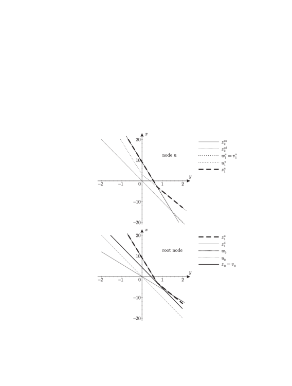
Figure 4.1: Algorithm 3.1 for the option seller in Example 4.1 at node $\mathrm{u}$ and the root node

The construction in Algorithm 3.2, equivalent by convex duality to Algorithm 3.1, is presented in Figure 4.2, also at node u and the root node. By examining the function $Z_{0}=z_{0}^{\ast}$ (which happens to have only one finite value in this example) we can also see that

$$\pi^{\mathrm{a}}(\xi,\zeta)=\max_{x\in\mathbb{R}}Z_{0}(x)=Z_{0}(10)=\textstyle 4\frac{1}{2}.$$

A mixed stopping time $\hat{\chi}\in\mathcal{X}$ and approximate martingale $(\hat{P},\hat{S})\in\mathcal{\bar{P}}(\hat{\chi})$ realising the seller’s price

$$\pi^{\mathrm{a}}(\xi,\zeta)=\mathbb{E}_{\hat{P}}((\xi+\hat{S}\zeta)_{\hat{\chi}})=\textstyle 4\frac{1}{2}$$

can be constructed as in Algorithm 3.4:

$$\begin{array}[c]{l}\hat{\chi}_{0}=0\\ \hat{P}_{0}=1\\ \hat{S}_{0}=10\end{array}\begin{array}[c]{l}\nearrow\\ \\ \\ \\ \searrow\end{array}\begin{array}[c]{l}\hat{\chi}_{1}^{\mathrm{u}}=\frac{3}{4}\\ \hat{P}_{1}^{\mathrm{u}}=1\\ \hat{S}_{1}^{\mathrm{u}}=8\\ \\ \\ \\ \\ \\ \hat{\chi}_{1}^{\mathrm{d}}=0\\ \hat{P}_{1}^{\mathrm{d}}=0\\ \hat{S}_{1}^{\mathrm{d}}=6\end{array}\begin{array}[c]{l}\nearrow\\ \searrow\\ \\ \\ \\ \\ \\ \\ \nearrow\\ \searrow\end{array}\begin{array}[c]{l}\hat{\chi}_{2}^{\mathrm{uu}}=\frac{1}{4}\\ \hat{P}_{2}^{\mathrm{uu}}=1\\ \hat{S}_{2}^{\mathrm{uu}}=16\\ \\ \hat{\chi}_{2}^{\mathrm{ud}}=\frac{1}{4}\\ \hat{P}_{2}^{\mathrm{ud}}=0\\ \hat{S}_{2}^{\mathrm{ud}}=10\\ \\ \hat{\chi}_{2}^{\mathrm{du}}=1\\ \hat{P}_{2}^{\mathrm{du}}=1\\ \hat{S}_{2}^{\mathrm{du}}=10\\ \\ \hat{\chi}_{2}^{\mathrm{dd}}=1\\ \hat{P}_{2}^{\mathrm{dd}}=0\\ \hat{S}_{2}^{\mathrm{dd}}=4\end{array}$$

This construction is also illustrated in Figure 4.2, which shows the values of the processes $\hat{S},\hat{X},\hat{Y},\hat{Z},\hat{U},\hat{V},\hat{W}$ at u and the root node. The values $\hat{\chi}_{0}=0$ and $\hat{\chi}_{1}^{\mathrm{u}}=\frac{3}{4}$ can be traced back to the following relationships, which can be seen in Figure 4.2:

$$\begin{array}[c]{cc}\hat{Y}_{0}=0\hat{S}_{0}+1\hat{X}_{0},&\hat{Y}_{1}^{\mathrm{u}}=\frac{3}{4}\hat{S}_{1}^{\mathrm{u}}+\frac{1}{4}\hat{X}_{1}^{\mathrm{u}},\\ \hat{Z}_{0}=0\hat{U}_{0}+1\hat{V}_{0},&\hat{Z}_{1}^{\mathrm{u}}=\frac{3}{4}\hat{U}_{1}^{\mathrm{u}}+\frac{1}{4}\hat{V}_{1}^{\mathrm{u}}.\end{array}$$

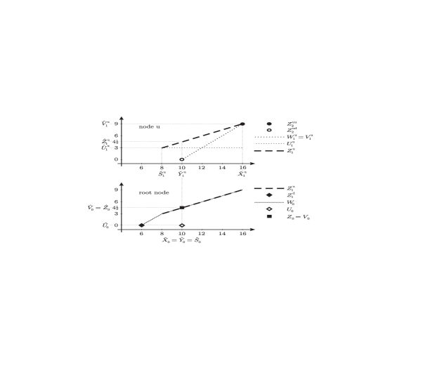
Figure 4.2: Algorithm 3.2 for the option seller in Example 4.1 at node $\mathrm{u}$ and the root node

This example also demonstrates that mixed stopping times play an essential role in the representation of the seller’s price $\pi^{\mathrm{a}}(\xi,\zeta)$ in Theorem 3.3, and cannot be replaced by pure stopping times. Indeed,

$$\max_{\tau\in\mathcal{T}}\max_{(P,S)\in\mathcal{\bar{P}}}\mathbb{E}_{P}(\xi_{\tau}+S_{\tau}\zeta_{\tau})=\textstyle 3\frac{3}{5},$$

attained for $\tau\equiv 2$, is lower than the seller’s price

$$\pi^{\mathrm{a}}(\xi,\zeta)=\max_{\chi\in\mathcal{X}}\max_{(P,S)\in\mathcal{\bar{P}}(\chi)}\mathbb{E}_{P}((\xi+S\zeta)_{\chi})=\textstyle 4\frac{1}{2}.$$

The buyer’s case, based on Algorithm 3.5, is shown in Figure 4.3. It involves non-convex functions such as $z_{1}^{\mathrm{u}}$ or $w_{0}$, hence there is no convex dual counterpart. The bid (buyer’s) price is

$$\pi^{\mathrm{b}}(\xi,\zeta)=-z_{0}(0)=\textstyle 1\frac{1}{5}.$$

The buyer’s optimal superhedging strategy $(\check{\alpha},\check{\beta})\in\Phi$ and optimal stopping time $\check{\tau}\in\mathcal{T}$ are constructed following Algorithm 3.6:

$$\begin{array}[c]{c}(\check{\alpha}_{0},\check{\beta}_{0})=\textstyle(-1\frac{1}{5},0)\end{array}\begin{array}[c]{c}\rightarrow\end{array}\begin{array}[c]{c}(\check{\alpha}_{1},\check{\beta}_{1})=\textstyle(1\frac{4}{5},-\frac{3}{10})\end{array}\begin{array}[c]{c}\nearrow\\ \searrow\end{array}\begin{array}[c]{l}(\check{\alpha}_{2}^{\mathrm{u}},\check{\beta}_{2}^{\mathrm{u}})=\textstyle(1\frac{4}{5},-\frac{3}{10})\\ \\ (\check{\alpha}_{2}^{\mathrm{d}},\check{\beta}_{2}^{\mathrm{d}})=\textstyle(1\frac{4}{5},-\frac{3}{10})\end{array}$$

$$\check{\tau}\equiv 1.$$

An approximate martingale $(\check{P},\check{S})\in\mathcal{\bar{P}}(\check{\tau})$ realising the buyer’s price

$$\pi^{\mathrm{b}}(\xi,\zeta)=\mathbb{E}_{\check{P}}(\xi_{\check{\tau}}+\check{S}_{\check{\tau}}\zeta_{\check{\tau}})=\min_{(P,S)\in\mathcal{\bar{P}}(\check{\tau})}\mathbb{E}_{P}(\xi_{\check{\tau}}+S_{\check{\tau}}\zeta_{\check{\tau}})$$

can be computed by applying Algorithm 3.4 to the option with payoff $(\xi_{t}^{\prime},\zeta_{t}^{\prime})=(-\xi_{t},-\zeta_{t})$ when $t=\check{\tau}$ and $(\xi_{t}^{\prime},\zeta_{t}^{\prime})=(-\infty,-\infty)$ when $t\neq\check{\tau}$ as explained in Section 3.2.3:

$$\begin{array}[c]{l}\check{P}_{0}=1\\ \check{S}_{0}=10\end{array}\begin{array}[c]{l}\nearrow\\ \\ \\ \searrow\end{array}\begin{array}[c]{l}\check{P}_{1}^{\mathrm{u}}=\frac{2}{5}\\ \check{S}_{1}^{\mathrm{u}}=16\\ \\ \\ \\ \\ \check{P}_{1}^{\mathrm{d}}=\frac{3}{5}\\ \check{S}_{1}^{\mathrm{d}}=6\end{array}\begin{array}[c]{l}\nearrow\\ \searrow\\ \\ \\ \\ \\ \nearrow\\ \searrow\end{array}\begin{array}[c]{l}\check{P}_{2}^{\mathrm{uu}}=\frac{2}{5}\\ \check{S}_{2}^{\mathrm{uu}}=16\\ \\ \check{P}_{2}^{\mathrm{ud}}=0\\ \check{S}_{2}^{\mathrm{ud}}=10\\ \\ \check{P}_{2}^{\mathrm{du}}=\frac{3}{5}\\ \check{S}_{2}^{\mathrm{du}}=10\\ \\ \check{P}_{2}^{\mathrm{dd}}=0\\ \check{S}_{2}^{\mathrm{dd}}=4\end{array}$$

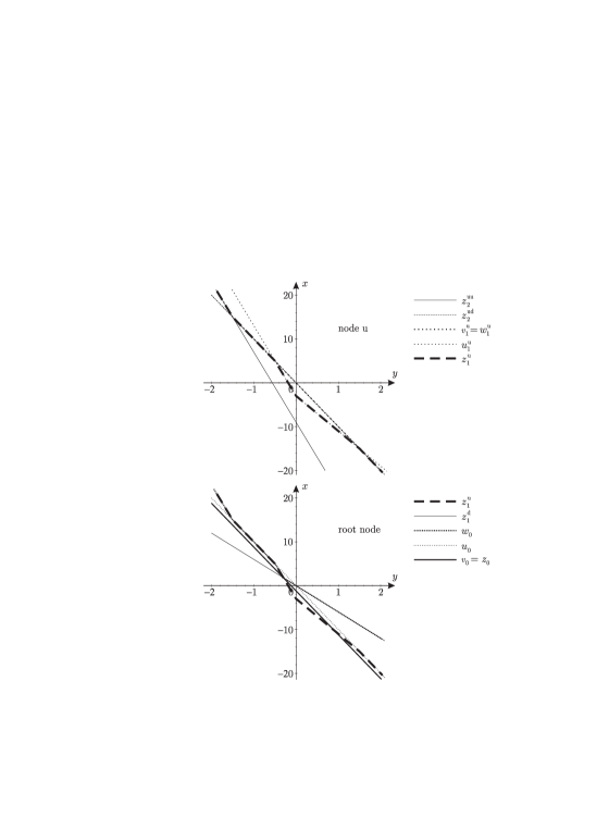
Figure 4.3: Algorithm 3.5 for the option buyer in Example 4.1 at node $\mathrm{u}$ and the root node

5 Numerical Results

In this section we extend the latest published numerical results in [PL04] for American puts under transaction costs very considerably and in various directions. The algorithms proposed in the present paper can handle not only American puts, but also arbitrary payoffs including option baskets, cover the full range of transaction costs, and are by no means restricted to the binomial model. The efficiency of the algorithms is reflected in the number of time steps in the numerical examples, larger than in [PL04] by more than an order of magnitude. This is made possible by the fact that in a recombinant model the computations in Algorithms 3.1 and 3.5 grow only polynomially with the number of time steps.

Example 5.1

This example is based on the setup in Perrakis and Lefoll [PL04] for an American put option in a binomial tree model under transaction costs. We reproduce the results in [PL04], and extend them to parameter ranges for which the small transaction costs assumption imposed in [PL04] (namely, condition (11) in that paper) is no longer satisfied. Thanks to the efficiency of Algorithms 3.1 and 3.5, we can cover a substantially larger number of time steps and larger transaction costs than in [PL04].

The stock price process $S$ in the binomial tree model is assumed to satisfy

$$S_{t}=\varepsilon_{t}S_{t-1}$$

for $t=1,\ldots,N$, with initial stock price $S_{0}=100$, and $\varepsilon_{1},\varepsilon_{2},\ldots$ a sequence of independent identically distributed random variables, each taking two possible values $e^{-\sigma\sqrt{T/N}}$ or $e^{\sigma\sqrt{T/N}}$ with positive probability, where $\sigma=0.2$ is the stock volatility, $T=0.25$ (three months), and $N$ is the number of time steps. We assume a continuously compounded interest rate of $10\%$, and a transaction cost rate $k\in[0,1)$ so that, for $t=1,\ldots,N$ the bid and ask stock prices are

$$S_{t}^{\mathrm{b}}=(1-k)S_{t},\quad S_{t}^{\mathrm{a}}=(1+k)S_{t}.$$

In line with [PL04], we also assume that no transaction costs apply at time $0$,

$$S_{0}^{\mathrm{b}}=S_{0}^{\mathrm{a}}=S_{0}.$$

We compute the ask (seller’s) and bid (buyer’s) prices of an American put option exercised by the physical delivery of a portfolio $(K,-1)$ of cash and stock, with strike price $K=100$ and time to expiry $T=0.25$. As in [PL04], the possibility that the option may never be exercised is included. Technically, in Algorithms 3.1 and 3.5 this is achieved by adding an extra time instant $N+1$ to the model and setting the option payoff to be $(0,0)$ at that time. For $N=20$ or $40$ time steps and transaction costs $k=0.5\%$ the results in Table 5.1 agree with those in Table 1 in [PL04]. The other results extend those in [PL04].

$\text{Number of time steps }(N)$ 20 40 100 250 500 1000 $k=0.00\%$ ask/bid 3.0485${}^{\mathrm{\phantom{a}}}$ 3.0596${}^{\mathrm{\phantom{ab}}}$ 3.0661${}^{\mathrm{\phantom{ab}}}$ 3.0685${}^{\mathrm{\phantom{ab}}}$ 3.0693${}^{\mathrm{\phantom{ab}}}$ 3.0697${}^{\mathrm{\phantom{ab}}}$ $k=0.25\%$ ask 3.4724^a 3.6366${}^{\mathrm{a\phantom{b}}}$ 3.9348${}^{\mathrm{a\phantom{b}}}$ 4.3691${}^{\mathrm{a\phantom{b}}}$ 4.8194${}^{\mathrm{a\phantom{b}}}$ 5.4023${}^{\mathrm{a\phantom{b}}}$ bid 2.5989^a 2.4074${}^{\mathrm{a\phantom{b}}}$ 1.9688${}^{\mathrm{a\phantom{b}}}$ 1.0772${}^{\mathrm{a\phantom{b}}}$ 0.0961${}^{\mathrm{a\phantom{b}}}$ 0.0319${}^{\mathrm{a\phantom{b}}}$ $k=0.50\%$ ask 3.8674${}^{\mathrm{\phantom{a}}}$ 4.1551${}^{\mathrm{\phantom{ab}}}$ 4.6761${}^{\mathrm{a\phantom{b}}}$ 5.4134${}^{\mathrm{a\phantom{b}}}$ 6.1544^ab 7.0876^ab bid 2.0917${}^{\mathrm{\phantom{a}}}$ 1.5975${}^{\mathrm{\phantom{ab}}}$ 0.2374${}^{\mathrm{a\phantom{b}}}$ 0.0612${}^{\mathrm{a\phantom{b}}}$ 0.0000^ab 0.0000^ab $k=1.00\%$ ask 4.5855^a 5.0695${}^{\mathrm{a\phantom{b}}}$ 5.9309^ab 7.1120^ab 8.2668^ab 9.6890^ab bid 0.6819^a 0.2589${}^{\mathrm{a\phantom{b}}}$ 0.0000^ab 0.0000^ab 0.0000^ab 0.0000^ab $k=2.00\%$ ask 5.8274^a 6.5985^ab 7.9437^ab 9.7499^ab 11.4706^ab 13.5544^ab bid 0.0492^a 0.0000^ab 0.0000^ab 0.0000^ab 0.0000^ab 0.0000^{ab a} Not in [PL04] ^b Small transaction costs condition (11) of [PL04] not satisfied

Table 5.1: American put prices in the binomial model of [PL04], Example 5.1

Example 5.2

Within the same binomial model of stock prices with transaction costs as in [PL04] described in Example 5.1 (with no transaction costs at time $0$) we consider an American bull spread, a basket consisting of a long call with strike price $95$ and a short call with strike price $105$. Assume that the bull spread is settled in cash, with payoff process $(S_{t}-95)^{+}-(S_{t}-105)^{+}$ and time to expiry $T=0.25$ (three months). The ask and bid prices of the bull spread are presented in Table 5.2.

$\text{Number of time steps }(N)$ 20 40 100 250 500 1000 $k=0.00\%$ ask/bid 7.1688 7.2519 7.2291 7.2023 7.2576 7.2361 $k=0.25\%$ ask 7.4267 7.5672 7.6538 7.8130 8.3572 8.5756 bid 6.8820 6.8793 6.6756 6.3090 5.9824 5.9202 $k=0.50\%$ ask 7.6616 7.8539 8.2783 8.6371 8.8761 8.9089 bid 6.5599 6.4183 5.8591 5.7264 5.7124 5.6683 $k=1.00\%$ ask 8.1274 8.5640 9.0392 9.1109 9.2269 9.2415 bid 5.7698 5.5778 5.3979 5.2908 5.2816 5.2413 $k=2.00\%$ ask 9.2537 9.4922 9.5584 9.5733 9.6343 9.6127 bid 5.0000 5.0000 5.0000 5.0000 5.0000 5.0000

Table 5.2: American bull spread prices in the binomial model, Example 5.2

Example 5.3

We take the same American bull spread as in Example 5.2, that is, a basket consisting of a long call with strike $95$ and a short call with strike $105$, both settled in cash and expiring at $T=0.25$ (three months), this time in the trinomial tree model with stock prices $S_{0}=100$ and

$$S_{t}=\varepsilon_{t}S_{t-1}$$

for $t=1,\ldots,N$, where $\varepsilon_{1},\ldots,\varepsilon_{N}$ are independent identically distributed random variables, each taking three possible values $e^{\sigma\sqrt{T/N}}$ or $1$ or $e^{-\sigma\sqrt{T/N}}$. The bid-ask spreads are defined in terms of the transaction cost rate $k\in[0,1)$

$$S_{t}^{\mathrm{b}}=(1-k)S_{t},\quad S_{t}^{\mathrm{a}}=(1+k)S_{t}$$

for all $t=1,\ldots,T$. By analogy to the binomial model in Examples 5.1 and 5.2, we assume that there are no transaction costs at time $0$, so that $S_{0}^{\mathrm{a}}=S_{0}^{\mathrm{b}}=S_{0}$. We take $\sigma=0.2$ and a continuously compounded interest rate of $10\%$. The ask and bid prices for this option computed by means of Algorithms 3.1 and 3.5 are presented in Table 5.3.

$\text{Number of time steps }(N)$ 20 40 100 250 500 1000 $k=0.00\%$ ask 7.4507 7.5825 7.6954 7.7718 7.8340 7.8702 bid 6.2780 6.3117 6.2696 6.2437 6.2977 6.2859 $k=0.25\%$ ask 7.8012 8.0152 8.2262 8.4083 8.5873 8.6322 bid 6.0191 6.0342 5.9580 5.8900 5.9054 5.8699 $k=0.50\%$ ask 8.1308 8.4095 8.6574 8.7313 8.8778 8.9090 bid 5.7705 5.7751 5.6739 5.6250 5.6509 5.6199 $k=1.00\%$ ask 8.7576 8.9660 9.0482 9.1110 9.2282 9.2415 bid 5.3123 5.3053 5.2201 5.1818 5.2100 5.1858 $k=2.00\%$ ask 9.3461 9.5141 9.5657 9.5733 9.6353 9.6127 bid 5.0000 5.0000 5.0000 5.0000 5.0000 5.0000

Table 5.3: American bull spread prices in the trinomial model, Example 5.3

6 Appendix: Technical Results

Proposition 6.1

For each $\chi\in\mathcal{X}$

$$\mathcal{P}\subset\mathcal{P}(\chi),\quad\mathcal{\bar{P}}\subset\mathcal{\bar{P}}(\chi).$$

Proof  To prove that $\mathcal{P}\subset\mathcal{P}(\chi)$, take any $(P,S)\in\mathcal{P}$ and any $\chi\in\mathcal{X}$. Because $S_{t}^{\mathrm{b}}\leq S_{t}\leq S_{t}^{\mathrm{a}}$, it is sufficient to show that for each $t=0,1,\ldots,T$

$$\chi_{t+1}^{\ast}S_{t}=\mathbb{E}_{P}(S_{t+1}^{\chi^{\ast}}|\mathcal{F}_{t}).$$ (6.1)

We proceed by backward induction. For $t=T$ both sides of (6.1) are equal to zero. Suppose that (6.1) holds for some $t=1,\ldots,T$. Then, since $\chi^{\ast}$ is a predictable process and $S$ is a martingale under $P$,

$$\mathbb{E}_{P}(S_{t}^{\chi^{\ast}}|\mathcal{F}_{t-1}) =\mathbb{E}_{P}(\chi_{t}S_{t}+S_{t+1}^{\chi^{\ast}}|\mathcal{F}_{t-1})=\mathbb{E}_{P}(\chi_{t}S_{t}+\mathbb{E}_{P}(S_{t+1}^{\chi^{\ast}}|\mathcal{F}_{t})|\mathcal{F}_{t-1})$$

$$=\mathbb{E}_{P}(\chi_{t}S_{t}+\chi_{t+1}^{\ast}S_{t}|\mathcal{F}_{t-1})=\mathbb{E}_{P}(\chi_{t}^{\ast}S_{t}|\mathcal{F}_{t-1})=\chi_{t}^{\ast}\mathbb{E}_{P}(S_{t}|\mathcal{F}_{t-1})$$

$$=\chi_{t}^{\ast}S_{t-1},$$

completing the induction step. The proof that $\mathcal{\bar{P}}\subset\mathcal{\bar{P}}(\chi)$ is very similar.  

Proposition 6.2

Let $(\alpha,\beta)\in\Phi$ be a superhedging strategy for the seller of an American option with payoff process $(\xi,\zeta)$. Then for every $\chi\in\mathcal{X}$ and every $(P,S)\in\mathcal{\bar{P}}(\chi)$

$$\mathbb{E}_{P}(\left(\xi+S\zeta\right)_{\chi})\leq-\vartheta_{0}(-\alpha_{0},-\beta_{0}).$$

Proof  The self-financing condition (2.1) satisfied by $\left(\alpha,\beta\right)$, along with inequalities (2.4), (2.5) from the definition of $\mathcal{\bar{P}}(\chi)$ imply that

$$\mathbb{E}_{P}(\chi_{t+1}^{\ast}\alpha_{t}+S_{t+1}^{\chi^{\ast}}\beta_{t}|\mathcal{F}_{t})\geq\mathbb{E}_{P}(\chi_{t+1}^{\ast}\alpha_{t+1}+S_{t+1}^{\chi^{\ast}}\beta_{t+1}|\mathcal{F}_{t})$$ (6.2)

for each $t=0,1,\ldots,T$. We shall prove by backward induction that

$$\mathbb{E}_{P}(\chi_{t}^{\ast}\alpha_{t}+S_{t}^{\chi^{\ast}}\beta_{t}|\mathcal{F}_{t})\geq\mathbb{E}_{P}((\alpha+S\beta)_{t}^{\chi^{\ast}}|\mathcal{F}_{t})$$ (6.3)

for each $t=0,1,\ldots,T$. Inequality (6.3) holds for $t=T$ since both sides are equal to $\chi_{T}(\alpha_{T}+S_{T}\beta_{T})$. Suppose that (6.3) holds for some $t=1,\ldots,T$. Then by (6.2)

$$\mathbb{E}_{P}(\chi_{t-1}^{\ast}\alpha_{t-1} +S_{t-1}^{\chi^{\ast}}\beta_{t-1}|\mathcal{F}_{t-1})$$

$$=\chi_{t-1}(\alpha_{t-1}+S_{t-1}\beta_{t-1})+\mathbb{E}_{P}(\chi_{t}^{\ast}\alpha_{t-1}+S_{t}^{\chi^{\ast}}\beta_{t-1}|\mathcal{F}_{t-1})$$

$$\geq\chi_{t-1}(\alpha_{t-1}+S_{t-1}\beta_{t-1})+\mathbb{E}_{P}(\chi_{t}^{\ast}\alpha_{t}+S_{t}^{\chi^{\ast}}\beta_{t}|\mathcal{F}_{t-1})$$

$$=\chi_{t-1}(\alpha_{t-1}+S_{t-1}\beta_{t-1})+\mathbb{E}_{P}(\mathbb{E}_{P}(\chi_{t}^{\ast}\alpha_{t}+S_{t}^{\chi^{\ast}}\beta_{t}|\mathcal{F}_{t})|\mathcal{F}_{t-1})$$

$$\geq\chi_{t-1}(\alpha_{t-1}+S_{t-1}\beta_{t-1})+\mathbb{E}_{P}(\mathbb{E}_{P}((\alpha+S\beta)_{t}^{\chi^{\ast}}|\mathcal{F}_{t})|\mathcal{F}_{t-1})$$

$$=\chi_{t-1}(\alpha_{t-1}+S_{t-1}\beta_{t-1})+\mathbb{E}_{P}((\alpha+S\beta)_{t}^{\chi^{\ast}}|\mathcal{F}_{t-1})$$

$$=\mathbb{E}_{P}((\alpha+S\beta)_{t-1}^{\chi^{\ast}}|\mathcal{F}_{t-1}),$$

completing the proof of (6.3). In particular, since $\chi_{0}^{\ast}=1$ and $\mathbb{E}_{P}(S_{0}^{\chi^{\ast}})=\mathbb{E}_{P}(S_{\chi})$, inequality (6.3) for $t=0$ implies that

$$\alpha_{0}+\mathbb{E}_{P}(S_{\chi})\beta_{0}=\mathbb{E}_{P}(\chi_{0}^{\ast}\alpha_{0}+S_{0}^{\chi^{\ast}}\beta_{0})\geq\mathbb{E}_{P}((\alpha+S\beta)_{0}^{\chi^{\ast}})=\mathbb{E}_{P}((\alpha+S\beta)_{\chi}).$$

Because $S_{0}^{\mathrm{b}}\leq\mathbb{E}_{P}(S_{\chi})\leq S_{0}^{\mathrm{a}}$, we have $-\vartheta_{0}(-\alpha_{0},-\beta_{0})\geq\alpha_{0}+\mathbb{E}_{P}(S_{\chi})\beta_{0}$. Since $(\alpha,\beta)$ is a superhedging strategy for the seller,

$$\vartheta_{t}(\alpha_{t}-\xi_{t},\beta_{t}-\zeta_{t})\geq 0.$$

This, together with the inequalities $S_{t}^{\mathrm{b}}\leq S_{t}\leq S_{t}^{\mathrm{a}}$, gives $\alpha_{t}+S_{t}\beta_{t}\geq\xi_{t}+S_{t}\zeta_{t}$. It follows that $(\alpha+S\beta)_{\chi}\geq(\xi+S\zeta)_{\chi}$ for each $t=0,1,\ldots,T$. We therefore obtain

$$-\vartheta_{0}(-\alpha_{0},-\beta_{0})\geq\alpha_{0}+\mathbb{E}_{P}(S_{\chi})\beta_{0}\geq\mathbb{E}_{P}((\alpha+S\beta)_{\chi})\geq\mathbb{E}_{P}((\xi+S\zeta)_{\chi}),$$

as claimed.  

Proposition 6.3

Let $(\xi,\zeta)$ be the payoff process of an American option. Then for any $\delta>0$, any mixed stopping time $\chi\in\mathcal{X}$ and any $(\bar{P},\bar{S})\in\mathcal{\bar{P}}(\chi)$ there exists a pair $(P^{\delta},S^{\delta})\in\mathcal{P}(\chi)$ such that

$$\left|\mathbb{E}_{P^{\delta}}((\xi+S^{\delta}\zeta)_{\chi})-\mathbb{E}_{\bar{P}}((\xi+\bar{S}\zeta)_{\chi})\right|<\delta.$$ (6.4)

Proof  Due to the lack of arbitrage, by the result of Jouini and Kallal [JK95], there exists some $(P,S)\in\mathcal{P}$. If $\mathbb{E}_{P}((\xi+S\zeta)_{\chi})=\mathbb{E}_{\bar{P}}((\xi+\bar{S}\zeta)_{\chi})$, then (6.4) is trivial because $\mathcal{P}\subset\mathcal{P}(\chi)$. If this is not the case, take any $\varepsilon$ such that

$$0<\varepsilon<\min\left\{1,\frac{\delta}{\left|\mathbb{E}_{P}\left((\xi+S\zeta)_{\chi}\right)-\mathbb{E}_{\bar{P}}\left((\xi+\bar{S}\zeta)_{\chi}\right)\right|}\right\},$$

and put

$$P^{\delta} =(1-\varepsilon)\bar{P}+\varepsilon P,$$

$$S_{t}^{\delta} =\mathbb{E}_{P^{\delta}}\!\!\left(\left.(1-\varepsilon)\bar{S}_{t}\frac{d\bar{P}}{dP^{\delta}}+\varepsilon S_{t}\frac{dP}{dP^{\delta}}\right|\mathcal{F}_{t}\right)$$

for each $t=0,1,\ldots,T$. It follows that $P^{\delta}$ is a probability measure equivalent to $Q$. It also follows that

$$S_{t}^{\delta}\leq S_{t}^{\mathrm{a}}\mathbb{E}_{P^{\delta}}\!\!\left(\left.(1-\varepsilon)\frac{d\bar{P}}{dP^{\delta}}+\varepsilon\frac{dP}{dP^{\delta}}\right|\mathcal{F}_{t}\right)=S_{t}^{\mathrm{a}}$$

and, in a similar way, that

$$S_{t}^{\mathrm{b}}\leq S_{t}^{\delta}$$

for any $t=0,1,\ldots,T$. Next,

$$\mathbb{E}_{P^{\delta}}((S^{\delta})_{t+1}^{\chi^{\ast}}|\mathcal{F}_{t})$$

$$\quad\quad=(1-\varepsilon)\mathbb{E}_{P^{\delta}}\!\!\left(\left.\bar{S}_{t+1}^{\chi^{\ast}}\frac{d\bar{P}}{dP^{\delta}}\right|\mathcal{F}_{t}\right)+\varepsilon\mathbb{E}_{P^{\delta}}\!\!\left(\left.S_{t+1}^{\chi^{\ast}}\frac{dP}{dP^{\delta}}\right|\mathcal{F}_{t}\right)$$

$$\quad\quad=(1-\varepsilon)\mathbb{E}_{\bar{P}}(\bar{S}_{t+1}^{\chi^{\ast}}|\mathcal{F}_{t})\mathbb{E}_{P^{\delta}}\!\!\left(\left.\frac{d\bar{P}}{dP^{\delta}}\right|\mathcal{F}_{t}\right)+\varepsilon\mathbb{E}_{P}(S_{t+1}^{\chi^{\ast}}|\mathcal{F}_{t})\mathbb{E}_{P^{\delta}}\!\!\left(\left.\frac{dP}{dP^{\delta}}\right|\mathcal{F}_{t}\right)$$

$$\quad\quad\leq\chi_{t+1}^{\ast}S_{t}^{\mathrm{a}}\left((1-\varepsilon)\mathbb{E}_{P^{\delta}}\!\!\left(\left.\frac{d\bar{P}}{dP^{\delta}}\right|\mathcal{F}_{t}\right)+\varepsilon\mathbb{E}_{P^{\delta}}\!\!\left(\left.\frac{dP}{dP^{\delta}}\right|\mathcal{F}_{t}\right)\right)=\chi_{t+1}^{\ast}S_{t}^{\mathrm{a}}$$

and, similarly,

$$\chi_{t+1}^{\ast}S_{t}^{\mathrm{b}}\leq\mathbb{E}_{P^{\delta}}((S^{\delta})_{t+1}^{\chi^{\ast}}|\mathcal{F}_{t})$$

for any $t=0,1,\ldots,T$. As a result, $(P^{\delta},S^{\delta})\in\mathcal{P}(\chi)$. Moreover,

$$\mathbb{E}_{P^{\delta}}((\xi+S^{\delta}\zeta)_{\chi}) =\mathbb{E}_{P^{\delta}}(\xi_{\chi})+\mathbb{E}_{P^{\delta}}((S^{\delta}\zeta)_{\chi})$$

$$=(1-\varepsilon)\mathbb{E}_{\bar{P}}(\xi_{\chi})\mathbb{+\varepsilon E}_{P}(\xi_{\chi})+(1-\varepsilon)\mathbb{E}_{\bar{P}}((\bar{S}\zeta)_{\chi})+\varepsilon\mathbb{E}_{P}((S\zeta)_{\chi})$$

$$=(1-\varepsilon)\mathbb{E}_{\bar{P}}((\xi+\bar{S}\zeta)_{\chi})+\varepsilon\mathbb{E}_{P}((\xi+S\zeta)_{\chi}),$$

which implies that

$$\left|\mathbb{E}_{P^{\delta}}((\xi+S^{\delta}\zeta)_{\chi})-\mathbb{E}_{\bar{P}}((\xi+\bar{S}\zeta)_{\chi})\right|=\varepsilon\left|\mathbb{E}_{P}((\xi+S\zeta)_{\chi})-\mathbb{E}_{\bar{P}}((\xi+\bar{S}\zeta)_{\chi})\right|<\delta.$$

References

- [BC77] S. Baxter and R. Chacon, Compactness of stopping times, Z. Wahrsch. verw. Gebiete 40 (1977), 169–181.
- [BT05] B. Bouchard and E. Temam, On the hedging of American options in discrete time markets with proportional transaction costs, Electronic Journal of Probability 10 (2005), 746–760.
- [CJ01] P. Chalasani and S. Jha, Randomized stopping times and American option pricing with transaction costs, Math. Finance 1 (2001), 33–77.
- [CP04] G.M. Constantinides and S. Perrakis, Stochastic dominance bounds on American option prices in markets with frictions, Working paper, University of Chicago, 2004.
- [CPS07] G.-Y. Chen, K. Palmer, and Y.-C. Sheu, The least cost super replicating portfolio for short puts and calls in the Boyle-Vorst model with transaction costs, Review of Quantitative Finance and Accounting (2007), to appear.
- [CRS71] Y.S. Chow, H. Robbins, and D. Siegmund, Great expectations: The theory of optimal stopping, Houghton Mifflin, Boston, 1971.
- [CZ01] G.M. Constantinides and T. Zariphopoulou, Bounds on derivative prices in an intertemporal setting with proportional transaction costs and multiple securities, Math. Finance 11 (2001), 331–346.
- [DZ95] M.H.A. Davis and T. Zariphopoulou, American options and transaction fees, Mathematical Finance (M.H.A. Davis et al., eds.), IMA Volumes in Mathematics and Its Applications, vol. 65, Springer, New York, 1995, pp. 47–61.
- [JK95] E. Jouini and H. Kallal, Martingales and arbitrage in securities markets with transaction costs, J. Econom. Theory 66 (1995), 178–197.
- [JLR03] P. Jakubenas, S. Levental, and M. Ryznar, The super-replication problem via probabilistic methods, Ann. Appl. Probab. 13 (2003), 742–773.
- [Koc99] M. Kociński, Optimality of the replicating strategy for American options, Appl. Math. (Warsaw) 26 (1999), 93–105.
- [Koc01] , Pricing of the American option in discrete time with proportional transaction costs, Math. Methods Oper. Res. 53 (2001), 67–88.
- [KRS02] Y. Kabanov, M. Rásonyi, and C. Stricker, No arbitrage criteria for financial markets with efficient friction, Finance Stoch. 6 (2002), 371–382.
- [KRS03] , On the closedness of sums of convex cones in and the robust no-arbitrage property, Finance Stoch. 7 (2003), 403–411.
- [KS01] Y. Kabanov and C. Stricker, The Harrison-Pliska arbitrage pricing theorem under transaction costs, J. Math. Econ. 35 (2001), 185–196.
- [LS97] S. Levental and A.V. Skorohod, On the possibility of hedging options in the presence of transaction costs, Ann. Appl. Probab. 7 (1997), 410–443.
- [MV97] F. Mercurio and T.C.F. Vorst, Options pricing and hedging in discrete time with transaction costs, Mathematics of Derivative Securities (M.A.H. Dempster and S.R. Pliska, eds.), Cambridge University Press, Cambridge, UK, 1997, pp. 190–215.
- [Ort01] F. Ortu, Arbitrage, linear programming and martingales in securities markets with bid-ask spreads, Decis. Econom. Finance 24 (2001), no. 2, 79–105.
- [PL00] S. Perrakis and J. Lefoll, Option pricing and replication with transaction costs and dividends, J. Econom. Dynam. Control 24 (2000), 1527–1561.
- [PL04] , The American put under transaction costs, J. Econom. Dynam. Control 28 (2004), 915–935.
- [Roc97] R.T. Rockafellar, Convex analysis, Princeton University Press, Princeton, 1997.
- [Rou06] A. Roux, European and American options under proportional transaction costs, Ph.D. thesis, University of York, 2006.
- [Rut98] M. Rutkowski, Optimality of replication in the CRR model with transaction costs, Appl. Math. (Warsaw) 25 (1998), 29–53.
- [Sch04] W. Schachermayer, The fundamental theorem of asset pricing under proportional transaction costs in finite discrete time, Math. Fin. 14 (2004), 19–48.
- [Tok04] K. Tokarz, European and American option pricing under proportional transaction costs, Ph.D. thesis, University of Hull, 2004.
- [TZ06] K. Tokarz and T. Zastawniak, American contingent claims under small proportional transaction costs, J. Math. Econom. 43 (2006), 65–85.