Is mass loss along the red giant branch of globular clusters sharply peaked? The case of M3

Abstract

There is a growing evidence that several globular clusters must contain multiple stellar generations, differing in helium content. This hypothesis has helped to interpret peculiar unexplained features in their horizontal branches. In this framework we model the peaked distribution of the RR Lyr periods in M3, that has defied explanation until now. At the same time, we try to reproduce the colour distribution of M3 horizontal branch stars. We find that only a very small dispersion in mass loss along the red giant branch reproduces with good accuracy the observational data. The enhanced and variable helium content among cluster stars is at the origin of the extension in colour of the horizontal branch, while the sharply peaked mass loss is necessary to reproduce the sharply peaked period distribution of RR Lyr variables. The dispersion in mass loss has to be $\leq$ 0.003 M_⊙, to be compared with the usually assumed values of $\sim$ 0.02 M_⊙. This requirement represents a substantial change in the interpretation of the physical mechanisms regulating the evolution of globular cluster stars.

1 Introduction

Since the early ’70s the population distribution along the horizontal branch (HB) in globular clusters (GCs) has been interpreted in terms of a variation of the mass of the hydrogen–rich envelope on top of the helium core, left over by the red giant evolution. The star to star difference in the amount of the hydrogen–rich material was explained as due to the stochastic nature of the mass loss process (Rood, 1973). The main feature to be reproduced was the distribution in number of HB members among the red, variable and blue regions. This has been possible for a large part of the GC system, assuming an average mass loss along the red giant (RG) branch evolution of $\Delta$M $\sim$ 0.22 M_⊙, with a $\sigma\sim$ 0.02 M_⊙ (see, f.e. Lee, Demarque, & Zinn, 1994).

On the other hand, it has always been clear that a not negligible number of HBs could not be understood following this assumption. A special case was that of the exclusively blue HBs (a consistent percentage of the total GC number), for which an increase in mass loss, in age, in RG rotation etc., has been invoked, generally with not great success (Fusi Pecci et al., 1993). But there are HB distributions that defy any simple explanation: bimodal and trimodal distributions, extremely long blue tails, hot blue stars in metal rich clusters are the most impressive examples (e.g. Rich et al., 1997; Sosin et al., 1997; Ferraro et al., 1998).

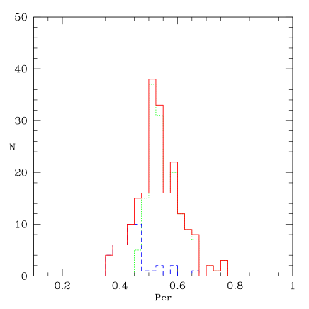
Figure 1: Period histogram (period in days) for M3 RR Lyrs from the data by Corwin & Carney 2001, where RRc have been fundamentalized (continuous red line); dotted green line: RRabs, dashed blue line: fundamentalized RRcs

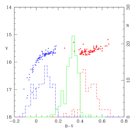
Figure 2: CM diagram of not-variable HB members M3 from the data by Corwin & Carney 2001 (not a complete sample, see text), with the histogram of their distribution with respect to B–V. Dashed (red) line: red HB members, dashed-dotted (blue) line: blue HB members; continuous (green) line: RR Lyrs histogram

Recently, the presence of peculiar patterns in the chemical abundances in many (if not all) GCs has provoked a renewed interest in the hypothesis of helium variations among globular cluster stars (Norris et al., 1981; Johnson & Bolte, 1998; D’Antona et al., 2002). The presence of more than one stellar generations, with differing helium contents, can explain features such as the multiple main sequences in $\omega$ Cen and NGC 2808 (Bedin et al., 2004; Norris, 2004; D’Antona et al., 2005; Lee et al., 2005; Piotto et al., 2005; Moehler & Sweigart, 2006; Piotto et al., 2007), the appearance of blue HB stars in metal rich GCs (e.g., NGC 6441, Caloi & D’Antona 2007), as well as of very blue and very faint HB members that are not understood in terms of ordinary evolutionary patterns (Brown et al., 2001).

So a new physical factor, the helium content, has begun to show a relevance comparable to that of mass loss in shaping HB morphology and population. At the same time, old unresolved riddles on HB star distribution, related in particular to some properties of the RR Lyr variables, have been recalled to attention. The attempts to solve these problems are imposing unexpected conditions on mass loss properties and on the role of varying helium content, so that we are possibly facing a rather substantial change of perspective in the interpretation both of the HB population and of the mass loss phenomenon during the RG ascent. This paper intends to expose this new point of view and some of its consequences.

2 M3, the horizontal branch and the RR Lyrae variables

The problem of the peaked distribution (see Fig. 1) of the RR Lyr periods in M3 (Castellani & Tornambe, 1981; Rood & Crocker, 1989) has been revisited by Catelan (2004) and Castellani et al. (2005). Catelan reached the conclusion that this feature cannot be understood in the framework of canonical HB evolution, while Castellani et al. found an interesting way to obtain the observed period distribution with current models. Their solution requires a strong constraint on mass loss, that has to have a very small dispersion ($\sigma$ $\sim$ 0.005 M_⊙) compared to normally accepted values ($\sigma$ $\sim$ 0.02 M_⊙). This occurrence allows the models to populate the RR Lyrae region just at the turning point of their blueward loops, with little dispersion, maximizing their permanence in the T_eff interval required to provide the peak in the period distribution. Anyway, these authors found two main difficulties with this modelization: i) a number of red HB stars noticeably larger than observed, and ii) the blue HB stars must be simulated by an ad hoc population, with a mean mass, and a $\sigma$ different from those required to explain the RR Lyr period distribution.

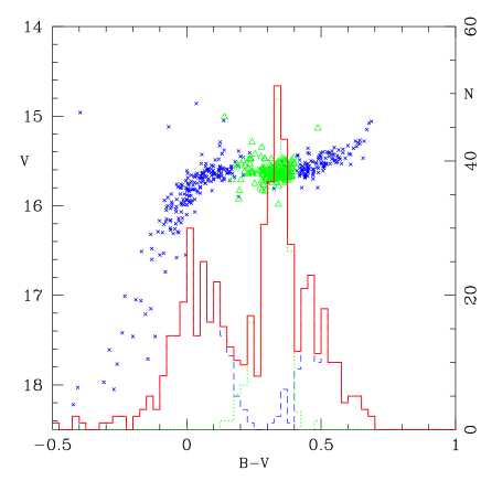
Figure 3: CM diagram of M3 from the data PH94 and CCD96 for the non variable stars (crosses, blue) plus the RR Lyrs by Corwin & Carney (triangles, green). Also shown is the histogram of their distribution with respect to B–V(continuous line, red); dashed line (blue): non variable stars, dotted (green) line: RR Lyr variables

In this paper we give a model for the period distribution of RR Lyrae variables in M3, following the suggestion of a very small mass dispersion for the mass loss along the RG branch. The extension in colour of the HB is then reproduced by assuming that the GC contains a second stellar generation with variable helium content, enhanced with respect to the first generation. For this cluster, while explaining in detail the HB morphology and the peaked period distribution of its RR Lyr, the scenario of multiple star generations provides a strong support to the rather surprising condition that mass loss must be sharply peaked.

3 The observational sample

At present we have periods, average magnitudes and colours for almost all the RR Lyrae variables in M3 (Benkő et al., 2006; Corwin & Carney, 2001). As guide to the details of M3 HB, we took the photometry by Corwin & Carney (2001), who give V, B–V for about 170 RR Lyr variables (and periods for 201), together with B, V photometry for blue and red HB members. The sample (and the corresponding histograms) shown in Fig. 2 is not complete since it shows only the stars with the best photometry (see Fig. 4 in Corwin & Carney), and we have limited the number of RR Lyrae variables to 100, roughly as expected from HB star counts in complete samples (see later). The importance of this sample is that it guarantees a uniform photometry all over the HB, and this is crucial to estimate the change in number density with colour when passing from the red to the variable and to the blue regions. From Fig. 2 we see that the number density grows passing from the red HB to the RR Lyrae region; then there is a dip in the population between variables and blue HB, followed by another peak at B–V $\sim$ 0.0 – 0.1. The dip in the colour distribution reproduces the paucity of stars in the RRc colour interval (specially at lower luminosity) and at the border of the blue region, clearly seen in Fig. 5 in Corwin & Carney paper. It is important to clarify that this dip is not affected by the well known uncertainties in the definition of the ”mean”colours for RR Lyr variables (see, f.e. Bono et al., 1995). In Fig. 2 we use magnitude average colours (B-V)_mag (Preston, 1961; Sandage, 1990), generally accepted as the best approximation to the colour of the ”static star” with the same average energy output. But any other common procedure would give the same result for RR Lyrs of type c, owing to their symmetric light curves (Bono et al., 1995), while possible differences up to 0.05 mag may be found for highly asymmetric light curves (as apply to RR Lyrs of type a). So the relative positions of RRc variables and constant blue HB stars can be considered as well established.

So any model for the star distribution along the HB must reproduce these two main features: the sharp peak in colour of the RR Lyraes (corresponding to the sharp peak in periods), and the dip in the population at the blue of the variables. Unfortunately, the Corwin & Carney (2001) HB sample is not complete. We then examined the complete samples from the CCD photometry by Ferraro et al. (1997) (CCD96) of the external cluster regions, and the photographic sample PH94 from Buonanno et al. (1994). The colours of the photographic sample turned out to be very similar, in the red and blue HB sections, to those in Corwin & Carney (2001), so that this sample guarantees a smooth continuity with the colours of the RR Lyrae. To obtain a larger complete sample, we include also the CCD photometric data by Ferraro et al. (1997), but we “corrected back” this photometry the PH94 photometry by using Equation 7 of the Ferraro et al. paper This correction is certainly not adequate for the bluest HB stars, which were not well measured on the photographic plates, but this is not an important point for our analysis, which is focused on the “horizontal” part of the HB. In Fig. 3 we show this complete sample (PH94, plus CCD96, plus the variables from Corwin & Carney (2001) with the related population histogram. The histogram for the variables is normalized to the number in the PH94 plus CCD96 samples as follows. The numbers we obtain for the red, variable and blue HB regions are 132, 222 and 217, respectively. This balance among the various populations is intermediate between what found for inner and outer regions by Catelan et al. (2001). In fact, they found a substantial difference between the population distributions for distances from the cluster center r $<$ 50” (28,65,81) and for r $>$ 120” (27,46,30). Given the uncertatinties involved, we shall consider our numbers as indicative of a substantial similarity between the variable and blue populations, while the red region is noticeably less populated than the variable one. As already pointed out by Castellani et al. (2005), and as we shall see in the following, this latter point represents one of the most difficult constraints with which the simulations have to comply.

Besides, we have to reproduce the RR Lyr period distribution and their mean period. The sharp peak in the period histogram (Fig. 1) descends from the colour distribution of the variables (Figs. 2 and 3); the mean period $\rm P_{\rm f}$ obtained fundamentalizing the RRc variables (addition of 0.128 to the logarithm of their periods, van Albada & Baker 1973) varies slightly with the chosen sample, and we assume $\rm P_{\rm f}$ to be comprised between 0.53 and 0.54 d. The sample by Corwin & Carney provides $\rm P_{\rm f}$ = 0.537 d.

4 The simulations

4.1 The models

We assume for the stars in M3 a heavy element content Z=0.001 and use our HB models descending from main sequence structures with $\rm Y_{\rm MS}$ =0.24, 0.28 and 0.32, as fully described in D’Antona & Caloi (2004). These models are the basis of the syntetic HBs computed in the following way. We fix a cluster age, and compute the evolving RG mass according to the relation (1) from D’Antona & Caloi (2004), which is a function of both age and Y. We assume that the stellar content of the cluster is divided into two main populations: a fraction of stars with cosmological helium (first generation), for which we assume Y=0.24, and the remaining fraction having larger and variable helium content (second generation). The number of the first generation stars, and the number vs. helium distribution of the second generation stars is changed in order to fit the whole HB. The HB mass is obtained by assuming that all RG stars lose an amount of mass $\delta$M, with a gaussian dispersion $\sigma$ around a fixed value $\delta$M₀. Then the HB mass varies both due to the mass dispersion $\sigma$ around the average assumed mass loss, and due to the dependence of the RG mass on the helium content. As the evolving mass decreases with increasing helium content, the stars with higher helium will populate bluer regions of the HB. In previous work (D’Antona & Caloi, 2004) we increased slightly the mass loss when increasing the helium content, following the idea that the global mass loss inversely depends on the stellar gravity, and so smaller masses would lose more mass (Lee, Demarque, & Zinn, 1994). Here we assume that the average mass lost is the same for all the helium contents. In fact, full evolutionary tracks including explicit consideration of mass loss, computed according to Reimers’ formulation, showed us that the total mass loss along the RG branch is independent of the helium content (at each given age): the track location and gravity compensate in such a way that the mass lost is constant at the level of 1-2$\times 10^{-3}$M_⊙, in most cases.

We assume a parametric mean mass loss along the RG branch with gaussian dispersion $\sigma$, and extract random both the mass loss and the HB age in the interval from 10⁶yr to 10⁸yr, according to the chosen Y distribution. We thus locate the luminosity and T_eff along the evolution of the HB mass obtained. These values are transformed into the observational plane M_v vs. B–V using Bessell, Castelli, & Plez (1998). We identify the variable stars as belonging to a fixed T_eff interval and compute their period according to the pulsation equation (1) by Di Criscienzo et al. (2004). The results are very similar if we adopt the classic van Albada & Baker (1973) relation. The real problem is given by the choice of the exact boundaries of the RR Lyr strip, that affect strongly the number and mean period of the RR Lyrae variables.

We assumed as width of the RR Lyr strip $\Delta$log$T_{\rm eff}$ = 0.08, a value commonly adopted (see, e.g., Castellani et al. 2005), and made a few experiments varying the choice of the red limit. We found that such limit had to be taken at log($T_{\rm eff}$) = 3.80, since for lower values a much larger than observed number of long period RRab’s (P $>$ 0.6 d) was present. Lower limits for the red edge temperature can be found in the literature (see the already quoted Catelan 2004 and Castellani et al. 2005). In order to avoid the presence of too many long period variables, Castellani et al. (2005) make use of decreased values of their model luminosities. We prefer to keep the theoretical values for the luminosity and adopt the correspondingly suitable value for the red edge.

One has also to consider that the estimate of the limiting temperatures is by no means a settled question. As discussed, e.g., by Di Criscienzo et al. (2004), the theoretical red edge of the pulsation region gets hotter by $\sim$ 300 K if the efficiency of superadiabatic convection in the star external layers is increased by changing the ratio mixing length to pressure scale height ($l/H_{\rm p}$) from 1.5 to 2. The comparison with observed periods shows that a larger convection efficiency should be preferred in several GCs (see Fig. 14 in Di Criscienzo et al. paper). At the same time, recent observational data also suggest hot values for the instability strip red boundary. Corwin et al. (1999) found for the colours of the RR Lyr variables in NGC 5466 (a very metal poor cluster) the limits 0.15 $<$ (B–V)₀ $<$ 0.38; similarly, Wehlau et al. (1999) found for NGC 7006, a GC with a Z close to that of M3, the limits 0.14 $<$ (B–V)₀ $<$0.38. Both these colour intervals correspond to T_eff intervals very close to our choice. Besides, Silbermann & Smith (1995), in their discussion of the blue and red edges in M15, say that the red edge may be near 6300 K.

We intend to reproduce the star distribution along the HB in some detail, not simply to obtain the overall distribution among red (R), variable (V) and blue (B) regions. To this purpose, the parameters we can play with are: i) the number of stars with cosmological Y (first stellar generation); ii) the number of stars with enhanced Y and their distribution as function of Y; iii) the mass loss and mass loss dispersion. The total number of stars involved is 571 (see above), to be distributed among helium contents from the cosmological one (Y = 0.24) up.

4.2 Results

On the basis of Fig. 2 and Fig. 3, it appeared reasonable to assume that the red HB and variable regions are populated mainly by stars with cosmological Y content, while blue HB members derive from smaller mass RG branch stars with a higher Y content, starting slightly above the cosmological one. evolving RG mass.

Once fixed the age and the heavy element content, for a given value of Y, the star distribution on the HB is decided by the amount of the mass loss on the RG branch. After few trials we could check that the only way to obtain peaked distributions of the variables in colour and period was to adopt a very well defined value for the mass loss. For an age of 11 Gyr and a population with initial Y content = 0.24, a peaked distribution in (B–V) (and period, see later) was obtained with a sharp mass loss value of $\Delta$(M) = 0.203 M_⊙, $\sigma$(M) $\leq$ 0.003 M_⊙. So the mass loss parameter turns out to be the most delicate and the less arbitrary among the ones mentioned before. We shall come back to this point.

In Fig. 4 we show a simulation of the HB distribution obtained with the quoted parameters, compared with the observed one. Some points are worth of attention. The simulation reproduces the main population peak in the RR Lyr region and the smaller one in the red section. It reproduces as well the dip at the blue of the RR Lyraes and the peak at B–V $\sim$ 0.0. The distribution in number along the HB gives 159 red members, 211 variable and 201 blue members, to be compared with the expected 132, 222 and 217 (see Sec. 3.1). Except for a slight excess of red stars (of the order of two $\sigma$), the similarity between the observed and the simulated distribution is remarkable. We stress that this is the first time that a detailed simulation has been attempted, since we tried to reproduce not simply the number of stars in the blue, variable and red HB regions, but the entire colour histogram of the HB population.

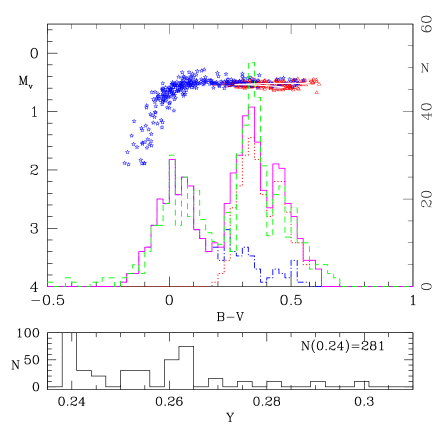
Figure 4: Simulation of the HB distribution (continuous magenta line) compared with the observed one (dashed green line, see Fig. 3); the dotted red line indicates the contribution by members with Y=0.24, the dashed-dotted blue line the contribution by members with enhanced Y, according to the distribution in Y shown in the lower panel. In white, the central track of the simulations.

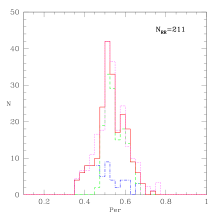
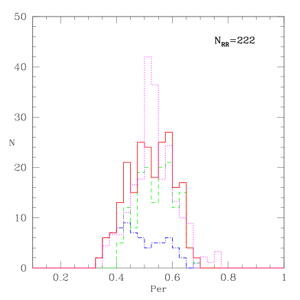
Figure 5: Simulated (continuous red line) and observed (dotted magenta line) period histograms; the contributions by members with Y=0.24 is indicated by the green dashed line, by members with enhanced helium by the blue dashed-dotted line. The number of “theoretical” RR Lyraes is reported. The left panel shows the simulation for $\sigma=0.0015$M_⊙, while the right panel shows the simulation for $\sigma=0.005$M_⊙. All other parameters are the same.

The left panel of Figure 5 shows the period histogram relative to the same simulation as in Fig. 4, compared with the observations (dotted line, see Fig. 1). The observational histogram of the RR Lyr periods has been obtained with a step of 0.025 d, which allows to appreciate the presence of a secondary peak in the distribution. We checked this feature comparing the histograms from the samples by Benkő et al. (2006) and by Corwin & Carney (2001), with an increasing step from 0.01 to 0.04 d. The two distributions appear very similar, and both show the presence of the secondary peak for steps $\leq$ 0.03 d, beyond which only the main peak is evident. Therefore, we consider this feature as well established, and an intriguing event that our simulation reproduces it. The agreement at the low and high limits for the period are also quite satisfactory, as well as the mean period. We think that the simultaneous satisfaction of so many observational requirements gives strong support to our basic choices.

Changing $\Delta$(M) from 0.203 M_⊙ to 0.201 or 0.205 M_⊙, the positions of the peaks in Figs. 4 and 5 appear slighlty shifted with respect to the observed distributions; in the case of a lower mass loss, one finds too many red stars ($\sim$ 170). We cannot exclude these values for what concerns the CM diagram, since the distribution in B–V cannot be considered completely determined (photometric imprecision, colour transformations). In any case, a small change in the absolute value of the mass loss does not affect the main point, that is, the need for a very small dispersion in mass loss, as discussed in the following.

The sharply peaked mass loss allows to have an almost unique value for the mass evolving through the RR Lyr region, and this is reflected in the peaked period distribution. A larger spread in mass loss will give rise to a larger spread in the masses evolving through the instability strip, and the sharp peak will be smoothed out.

To show how stringent is the assumption of a very small $\sigma$, the right panel of Figure 5 shows the period distribution for an identical simulation, differing only for the increase in $\sigma$ to 0.005 M_⊙. We see that the period distribution is much flatter and the peak had disappeared. We applied a Kolmogorov Smirnov (KS) test to the simulated and observed periods, to derive the probabilities that they are drawn from the same parent distributions. The simulation shown in the left panel has a probability of 89%, while this is reduced to 5% for the right panel. In order to prove that the situation in Fig. 5 is not peculiar, we applied the KS test to 500 simulations with $\sigma$=0.0015 as well as to 500 ones with $\sigma$=0.005. The simulations have strictly the same inputs, apart from the dispersion in mass loss. The probability that the observed and simulated periods are extracted from the same distribution is $>$50% for 379 cases (75%) when $\sigma$=0.0015, but only for 15 cases (3%) when $\sigma$=0.005. In the intermediate case of $\sigma$=0.003, we have probability $>$50% for 245 cases out of 500. In addition, remember that $\sigma$=0.005 is still a small mass loss dispersion indeed, to be compared with $\sigma$=0.02 commonly assumed to reproduce the color extension of HB stars in M3.

5 Discussion of the other simulation requirements

In building up a synthetic HB model with variable helium content, one might wonder how flexible (arbitrary?) is the choice of the number vs helium distribution. Actually, the distribution in number among the red and variable members on the one side, and the blue HB stars on the other, depends directly on the assumed number for the first generation (that is, with cosmological helium) stars. This number has to be lower than the sum of red and variable stars, because some helium-enriched stars will always populate these regions, even if originating on the blue side of the RR Lyr zone. In turn, these stars cannot be too many, otherwise the RRc region would turn out too populated, with also a decrease in the mean RR Lyr period. On the other hand, the first generation cannot be too numerous, otherwise the number of red stars largely exceeds the expected one.

The details of a helium distribution satisfying these conditions (being the parent of the simulation discussed in the paper) are reported in the lower panel of Fig. 4. While minor variations in the specific numbers would not be relevant, some characteristic features can be identified: i) the cluster population is equally divided between original (281) and enriched (290) helium abundances; ii) the bulk of the helium enriched population is around Y $\sim$ 0.26; iii) a tail with Y up to $\sim$ 0.30 may be necessary to explain most of the blue HB members (but we do not wish to put too much emphasis on this point).

Some stars (about 50) with 0.24 $\;\buildrel<\over{\sim}\;$ Y $\;\buildrel<\over{\sim}\;$ 0.245 appear in the helium distribution: they are necessary to avoid too large a dip in population between RR Lyr variables and blue HB stars. The same position on the HB would have been attained if we had assumed that these stars had Y = 0.24 and a slightly larger mass loss. The effect of an increase in Y from 0.24 to 0.245 is equivalent, for what concerns the resulting HB star mass, to an increase in the mass lost by an evolving giant, with Y = 0.24, from 0.203 to 0.210 M_⊙. A small asymmetry towards a larger mass loss would not be unexpected, and would be present in about 15% of the first stellar generation (50/331).

The amount of blue HB members is given roughly by the number of helium enhanced stars. As stressed before, there are no definite observational values for the relative numbers of red, variable and blue stars, and in any case the number of blue members can be easily accomodated varying the number of helium enhanced stars. If we exclude the 50 stars with 0.245$\leq$ Y $\leq$0.24, according to the latter hypothesis, we are left with $\sim$ 40% of stars with enhanced helium. This percentage is close to what we found for other GCs (D’Antona et al. 2006). However, in this case the helium distribution is peaked at the relatively small value of Y $\sim$ 0.26, compatible with the mild chemical anomalies observed in this cluster (Sneden et al. 2004).

As most of the HB members in Fig. 4 (90%) has Y $\leq$ 0.265, this ensures that the CM diagram of M3 is not expected to show peculiarities in the position of the main sequence, the turn–off, etc. In particular, the position of the GB bump will be very close to that expected for a purely cosmological Y content. In addition, the HB luminosity of the stars at the blue side of the RR Lyr region is only mildly affected by the enhanced helium, which at these locations is in the range 0.25$\;\buildrel<\over{\sim}\;$Y$\;\buildrel<\over{\sim}\;$0.26. This is shown in Figure 6, where on the observed HB are superimposed three tracks with Y=0.24, a track with Y=0.26 and one with Y=0.28. Maybe a better photometry could discriminate whether actually there is a helium enhancement at the blue side of the RR Lyrs.

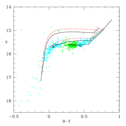
Figure 6: Tracks for standard helium Y=0.24, Z=0.001 and masses M=0.6588, 0.63 and 0.58 M_⊙ (from right to left, full lines) are superimposed to the observational HB data. The dashed (red) line is the M=0.63 M_⊙ track for Y=0.26, and the dot–dashed (red) line is the M=0.58 M_⊙ track for Y=0.28. The presence of slightly helium enhanced stars at the blue side of the RR Lyrs appears consistent with the data.

The problem of the red star number has been widely discussed in Castellani et al. (2005), who found by far too many stars of this kind. We are less plagued by this problem, but still the number of red stars in the simulations turns out most of the times larger than observed. It is not easy to think of a way out of this excess, given the strict conditions imposed by the RR Lyrae colour and period distribution. As mentioned before, the contribution to the variables by stars coming from the blue side cannot be too large because of the dip in population just at the blue of the RR Lyrae and in the RRc region (see Fig. 5 in Corwin & Carney 2001). Besides, too many variables coming from the blue would lower substantially the observed RR Lyr mean period. This question will be eaxamined in more detail in the following Section.

6 Discussion and conclusions

6.1 The global interpretation of the HB of M3

The extraordinary precision in the mass loss required by the simulations deserves some comments. In Fig. 4 it is shown the track of a HB star with a mass of 0.659 M_⊙, corresponding to the evolving giant of 11 Gyr (Z=0.001, Y=0.24) after a mass loss of 0.203 M_⊙. The two peaks in the histogram of the star distribution in the red and variable regions (Fig. 4) have a clear correspondence with the time development along the evolutionary track. The peak in the red region is given by the first evolutionary phases along the short redward loop and the turning toward the blue, while the peak in the RR Lyr region is the result of the slowing down of the evolution in colour during the bend of the track at the end of the blueward loop, with the beginning of the final movement to the red. The requirement of a small dispersion in mass is due to the necessity of keeping this pattern clear of the confusion that would arise mixing the evolutions of even a rather small mass spectrum.

Figures 4 and 5 show that RRc variables derive mainly from helium-enhanced stars, at the colour interval around the maximum blue extension of the 0.659 M_⊙ track. Here one finds also the dip in the star distribution at the RR Lyr blue limit, set by the colour limit of HB members with original helium content, and by the small difference in helium content among the first star generation and the succeeding ones. The dispersion along the blue HB, given the reduced dispersion in mass, is due to the dispersion in helium, as shown in the lower panel of Fig. 4.

In fact, there are two main differences between our analysis and the analysis by Castellani et al. (2005): i) they assume for the mass distribution which provides the RR Lyr variables a $\sigma=0.005$ M_⊙, while we have shown that our best matches with the period distribution are obtained by a $\sigma$ much smaller – almost a unique mass is evolving in the RR Lyr region; ii) they have to fill up the blue side of the HB with an ad hoc population, while we assume the model of a second stellar generation with varying helium content, as we have already done to interpret other complex HB distributions, such as in NGC 2808 (D’Antona & Caloi, 2004) and in NGC 6441 (Caloi & D’Antona, 2007). In this framework, our interpretation for the strong constraint on the mass loss rate along the RG is much more cogent.

6.2 A sharp value of mass loss also in other GCs?

The population distribution along the HB and the period distribution of the RR Lyr variables have been obtained assuming the presence of (at least) two populations with differing helium contents and, most important, an extremely narrow dispersion in the mass loss. This latter condition may be considered as necessarily requiring the presence of the first condition, since the blue HB population cannot be understood in terms of “one mass” evolution, as it happens for the red and variable members.

So the multiple star generations with varying Y hypothesis appears capable of coping with the rather strong condition of a very sharp amount of mass loss during RG evolution in M3 population. The variations in Y takes the place of the variations in mass, to explain the HB star distribution. We have seen already in other clusters similar situations. For example, in NGC 2808 (D’Antona & Caloi 2004) the red clump required a relatively small mass dispersion ($\sigma\simeq$ 0.015), and the long blue HB region was obtained with a distribution in Y. But the situation in M3 appears much more stringent in the requirement on mass loss, basically due to the RR Lyr properties that cannot be satisfied with a not–peaked mass distribution.

How special is the case of M3? The point has been discussed by Catelan (2004) and Castellani et al. (2005), who incline to consider M3 as perhaps a “pathological” case. They observe that M5 and M62, both rich in RR Lyr variables, show a less pronounced peak in the period distribution (see also Castellani et al. 2003, Fig. 1). While this is perhaps true, at least for M5, one finds in the quoted Fig. 1 (Castellani et al. 2003), many other Oosterhoff I clusters with about 70 RR variables (as in M62, according to Clement et al. 2001) with strongly peaked period distributions (NGC 6715, 6934, 7006). The problem with these clusters appears similar to that found in M3. Let us quote also the case of Palomar 3 (Catelan et al. 2001), that requires a very small mass dispersion (consistent with zero, according to the authors) to describe the HB distribution.

We think therefore that the problem is with us to stay. If the small dispersion in mass loss will be confirmed, we will face a rather impressive change of perspective in the interpretation of HB distributions. The role of the first phases of the dynamical and chemical evolution of GCs will become more and more crucial. In turn, these phases are dominated by the behaviour of the initial mass function, of the chemical processes in asymptotic giant branch stars and on their mass loss efficiency. So, on the one side we think that the hypothesis of multiple stellar generations begins to find a certain amount of observational support, and on the other we are well aware of the long way to reach an understanding of how such a phenomenon took place.

References

- Bedin et al. (2004) Bedin, L. R., Piotto, G., Anderson, J., Cassisi, S., King, I. R., Momany, Y., & Carraro, G. 2004, ApJ, 605, L125
- Benkő et al. (2006) Benkő, J. M., Bakos, G. Á., & Nuspl, J. 2006, MNRAS, 372, 1657
- Bessell, Castelli, & Plez (1998) Bessell, M. S., Castelli, F., & Plez, B. 1998, A&A, 333, 231
- Bono et al. (1995) Bono, G., Caputo, F., & Stellingwerf, R. F. 1995, ApJS, 99, 263
- Brown et al. (2001) Brown, T. M., Sweigart, A. V., Lanz, T., Landsman, W. B., & Hubeny, I. 2001, ApJ, 562, 368
- Buonanno et al. (1994) Buonanno, R., Corsi, C. E., Buzzoni, A., Cacciari, C., Ferraro, F. R., & Fusi Pecci, F. 1994, A&A, 290, 69
- Caloi & D’Antona (2007) Caloi, V., & D’Antona, F. 2007, A&A, 463, 949
- Castellani & Tornambe (1981) Castellani, V., & Tornambe, A. 1981, A&A, 96, 207
- Castellani et al. (2003) Castellani, M., Caputo, F., & Castellani, V. 2003, A&A, 410, 871
- Castellani et al. (2005) Castellani, M., Castellani, V., & Cassisi, S. 2005, A&A, 437, 1017
- Catelan et al. (2001) Catelan, M., Ferraro, F. R., & Rood, R. T. 2001, ApJ, 560, 970
- Catelan (2004) Catelan, M. 2004, ApJ, 600, 409
- Clement et al. (2001) Clement, C. M., et al. 2001, AJ, 122, 2587
- Corwin & Carney (2001) Corwin, T. M., & Carney, B. W. 2001, AJ, 122, 3183
- Corwin et al. (1999) Corwin, T. M., Carney, B. W., & Nifong, B. G. 1999, AJ, 118, 2875
- D’Antona et al. (2002) D’Antona, F., Caloi, V., Montalbán, J., Ventura, P., & Gratton, R. 2002, A&A, 395, 69
- D’Antona & Caloi (2004) D’Antona, F., & Caloi, V. 2004, ApJ, 611, 871
- D’Antona et al. (2005) D’Antona, F., Bellazzini, M., Caloi, V., Fusi Pecci, F., Galleti, S., & Rood, R. T. 2005, ApJ, 631, 868
- D’Antona et al. (2006) D’Antona, F., Ventura, P., & Caloi, V. 2006, invited talk at the Conference: From Stars to Galaxies: Building the Pieces to Build up the Universe, Venice, Astronomical Society of the Pacific Conference Series, Eds. A. Vallenari, R. Tantalo,.L. Portinari and A. Moretti, in press, ArXiv Astrophysics e-prints, arXiv:astro-ph/0612654
- Di Criscienzo et al. (2004) Di Criscienzo, M., Marconi, M., & Caputo, F. 2004, ApJ, 612, 1092
- Ferraro et al. (1998) Ferraro, F. R., Paltrinieri, B., Pecci, F. F., Rood, R. T., & Dorman, B. 1998, ApJ, 500, 311
- Ferraro et al. (1997) Ferraro, F. R., Carretta, E., Corsi, C. E., Fusi Pecci, F., Cacciari, C., Buonanno, R., Paltrinieri, B., & Hamilton, D. 1997, A&A, 320, 757
- Fusi Pecci et al. (1993) Fusi Pecci, F., Ferraro, F. R., Bellazzini, M., Djorgovski, S., Piotto, G., & Buonanno, R. 1993, AJ, 105, 1145
- Gratton et al. (2001) Gratton, R. G. et al. 2001, A&A, 369, 87
- Johnson & Bolte (1998) Johnson, J. A., & Bolte, M. 1998, AJ, 115, 693
- Lee, Demarque, & Zinn (1994) Lee, Y., Demarque, P., & Zinn, R. 1994, ApJ, 423, 248
- Lee et al. (2005) Lee, Y.-W., et al. 2005, ApJ, 621, L57
- Moehler & Sweigart (2006) Moehler, S., & Sweigart, A. V. 2006, A&A, 455, 943
- Norris et al. (1981) Norris, J., Cottrell, P. L., Freeman, K. C., & Da Costa, G. S. 1981, ApJ, 244, 205
- Norris (2004) Norris, J. E. 2004, ApJ, 612, L25
- Piotto et al. (2005) Piotto, G., et al. 2005, ApJ, 621, 777
- Piotto et al. (2007) Piotto, G., et al. 2007, ArXiv Astrophysics e-prints, arXiv:astro-ph/0703767
- Preston (1961) Preston, G. 1961, ApJ, 133, 29
- Reimers (1977) Reimers, D. 1977, A&A, 61, 217
- Rich et al. (1997) Rich, R. M., et al. 1997, ApJ, 484, L25
- Rood (1973) Rood, R. T. 1973, ApJ, 184, 815
- Rood & Crocker (1989) Rood, R. T., & Crocker, D. A. 1989, IAU Colloq. 111: The Use of pulsating stars in fundamental problems of astronomy, 103
- Sandage (1990) Sandage, A. 1990, ApJ, 350, 603
- Sneden et al. (2004) Sneden, C., Kraft, R. P., Guhathakurta, P., Peterson, R. C., & Fulbright, J. P. 2004, AJ, 127, 2162
- Silbermann & Smith (1995) Silbermann, N. A., & Smith, H. A. 1995, AJ, 110, 704
- Sosin et al. (1997) Sosin, C., et al. 1997, ApJ, 480, L35
- van Albada & Baker (1973) van Albada, T. S., & Baker, N. 1973, ApJ, 185, 477
- Ventura et al. (2001) Ventura, P., D’Antona, F., Mazzitelli, I., & Gratton, R. 2001, ApJ, 550, L65
- Ventura, D’Antona, & Mazzitelli (2002) Ventura, P., D’Antona, F., & Mazzitelli, I. 2002, A&A, 393, 215
- Ventura & D’Antona (2005a) Ventura, P., & D’Antona, F. 2005a, A&A, 431, 279
- Ventura & D’Antona (2005b) Ventura, P., & D’Antona, F. 2005b, ApJ, 635, L149
- Wehlau et al. (1999) Wehlau, A., Slawson, R. W., & Nemec, J. M. 1999, AJ, 117, 286