A dynamic density functional theory for particles in a flowing solvent

Abstract

We present a dynamic density functional theory (dDFT) which takes into account the advection of the particles by a flowing solvent. For potential flows we can use the same closure as in the absence of solvent flow. The structure of the resulting advected dDFT suggests that it could be used for non-potential flows as well. We apply this dDFT to Brownian particles (e.g., polymer coils) in a solvent flowing around a spherical obstacle (e.g., a colloid) and compare the results with direct simulations of the underlying Brownian dynamics. Although numerical limitations do not allow for an accurate quantitative check of the advected dDFT both show the same qualitative features. In contrast to previous works which neglected the deformation of the flow by the obstacle, we find that the bow–wave in the density distribution of particles in front of the obstacle as well as the wake behind it are reduced dramatically. As a consequence the friction force exerted by the (polymer) particles on the colloid can be reduced drastically.

I Introduction

The generalization of classical density functional theory (DFT) to non-equilibrium states has become a valuable tool to study the dynamics of interacting Brownian particles. This dynamic density functional theory (dDFT) for the ensemble averaged density was proposed recently in Marconi and Tarazona (1999, 2000). Although hydrodynamics is known to play a crucial role in the dynamics of suspensions, dDFT has also been used to describe colloidal suspensions or polymer solutions, in particular to investigate the distribution of solute particles around a strongly repulsive potential moving through the solution of particles Penna et al. (2003). The intention was to model a colloidal particle moving through a polymer solution. A similar model has been used to study the depletion interaction between two colloidal particles moving through a polymer solution Dzubiella et al. (2003); Krüger and Rauscher (2007). In all these studies the hydrodynamic flow of the solvent around the colloid was neglected and the solvent effectively passed through the colloid. A real colloid would displace the solvent as it moves, as shown for the case of a small and a large colloid in Fig. 1. For a spherical colloidal particle of radius $R$ dragged through an unbounded incompressible viscous Newtonian solvent with velocity $\mathbf{c}$ at low Reynolds number, the flow field $\mathbf{u}(\mathbf{r})$ (in a frame of reference comoving with the colloid) is given by the solution of the Stokes equation Landau and Lifshitz (2005),

$$\mathbf{u}(\mathbf{r})=\frac{3\,R}{4\,r}\,\left(1+\frac{R^{2}}{3\,r^{2}}\right)\,\mathbf{c}+\frac{3\,R}{4\,r^{3}}\,\mathbf{r}\,(\mathbf{r}\cdot\mathbf{c})\,\left(1-\frac{R^{2}}{r^{2}}\right)-\mathbf{c}.$$ (1)

For large distances from the colloid, $r\gg R$, the flow field is well approximated by $\mathbf{u}(\mathbf{r})=-\mathbf{c}$. For solute particles (e.g., polymers or other colloids) which only feel this far field, the model presented in Penna et al. (2003); Dzubiella et al. (2003); Krüger and Rauscher (2007) is a reasonable approximation. This is the case for large solute particles with a radius $d\gg R$. Their centers can approach the dragged colloidal particle only up to a distance $D=R+d\approx d$, see Fig. 1(a), and thus will feel a flow field $\mathbf{u}(\mathbf{r})\approx-\mathbf{c}$, if one neglects the additional effect of the solute particles on the solvent flow, in other words, the hydrodynamic interaction between the solute particle and the colloid is neglected. This is a reasonable approximation for polymer coils but certainly a bad one for solid solute particles. But small solute particles of radius $d\ll R$ can get much closer to the colloid and feel the distortion of the solvent velocity field as illustrated in Fig. 1(b). The solute particles will be deviated from the colloid by the flow field and this will reduce significantly the bow–wave effect in front of the colloid presented in Penna et al. (2003) and the strenght of the non-equilibrium depletion force discussed in Dzubiella et al. (2003); Krüger and Rauscher (2007). Extremely small solute particles would not show this effect at all since they would behave like solvent molecules. In this limit, however, the basis of the theory discussed here, i.e, the description of the solute particles as overdamped Brownian particles, is no longer valid because it is based on a separation of the length and time scales associated with the solvent molecules and the solute particles.

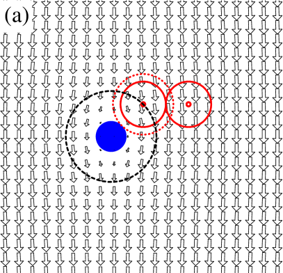
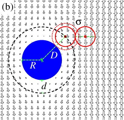
Figure 1: Cross section of the flow field given by Eq. (1) in a plane parallel to the direction of motion around (a) a small spherical colloid and (b) a big one (full circles, radius $R$). The dashed circles of radius $D$ mark the points of closest approach of solute’s centers (point in the center of open circles) to the colloid. The solute’s diameter in its mutual interaction is $\sigma$ and, for non-additive mixtures, not necessarily equal to its diameter $2\,d=2\,(D-R)$ (indicated by the dotted circle) in the interaction with the colloid. The component of the flow field normal to the dashed circle is larger for the small colloid (a) than for the large colloid (b). $\sigma$ and $d$ are the same in both figures.

In this paper we present a generalization of the dDFT derived in Marconi and Tarazona (1999, 2000) to the case of Brownian solvent particles advected by a flow, thereby incorporating some aspects of the hydrodynamics of the solvent into the theory. However, we do not model hydrodynamic interactions between the solute particles as well as the back-reaction of the solute particles on the flow field, e.g., by a concentration dependent viscosity, or by a reduced mobility of the solute particles in the vicinity of the colloid. However, the latter can be included in a straightforward manner as we discuss in the conclusions in Sec. IV. In the following Sec. II we derive the advected dynamic density functional theory using the method described in Archer and Evans (2004); Archer and Rauscher (2004). In Sec. III we discuss two sample cases, namely ideal solute particles and Gaussian solute particles which stress the importance of taking into account the solvent flow.

II Advected dDFT

We start with the Langevin equation of an ensemble of $N$ advected interacting Brownian particles confined to a finite volume $\mathcal{V}$ in the overdamped limit,

$$\frac{d\mathbf{r}_{i}}{dt}=\mathbf{u}(\mathbf{r}_{i})-\Gamma\,\bm{\nabla}_{i}\left[U(\mathbf{r}_{i})+\sum\limits_{j=1}^{N}V(|\mathbf{r}_{i}-\mathbf{r}_{j}|)\right]+\bm{\eta}_{i}(t),$$ (2)

with the pair interaction potential between the particles $V(r)$ and an external potential $U(\mathbf{r})$. Both the external potential $U(\mathbf{r})$ and the flow field $\mathbf{u}(\mathbf{r})$ can depend on time. For clarity of notation we will not make this dependence explicit in the equations. The flow field is not necessarily divergence free (i.e., the solvent can be compressible). $\bm{\nabla}_{i}$ denotes the gradient with respect to $\mathbf{r}_{i}$. We approximate the noise generated by the thermal motion of the solvent particles by a Wiener process,

$$\langle\bm{\eta}_{i}(t)\rangle =\bm{0}\quad\quad\quad\text{and}$$ (3)

$$\langle\eta_{i}^{\alpha}(s)\,\eta_{j}^{\beta}(t)\rangle =2\,T\,\Gamma\,\delta_{ij}\,\delta_{\alpha\beta}\,\delta(t-s),$$ (4)

with the temperature $T$ measured in units of energy (setting $k_{\!B}=1$) and the mobility coefficient $\Gamma>0$. The mobility coefficient has to appear in the correlation in Eq. (4) in order to fulfill the fluctuation–dissipation theorem and to get the correct equilibrium distribution for $\mathbf{u}(\mathbf{r})=\bm{0}$. The boundaries of $\mathcal{V}$ are impermeable for the particles or periodic (or a mixture of both), and therefore the number of particles is conserved.

The Fokker-Planck equation corresponding to the Langevin equation (2) gives the time evolution of the probability density $W(\mathbf{r}_{1},\dots,\mathbf{r}_{N},t)$ for finding the particles at time $t$ at the positions $\mathbf{r}_{1},\dots,\mathbf{r}_{N}$ Gardiner (1983); Risken (1984),

$$\frac{\partial W}{\partial t}=-\sum\limits_{i=1}^{N}\bm{\nabla}_{i}\cdot\Bigg{\{}\Gamma\Bigg{[}\frac{\mathbf{u}(\mathbf{r}_{i})}{\Gamma}-\bm{\nabla}_{i}U(\mathbf{r}_{i})\\ -\sum\limits_{j=1}^{N}\bm{\nabla}_{i}V(|\mathbf{r}_{i}-\mathbf{r}_{j}|)-T\,\bm{\nabla}_{i}\Bigg{]}\,W\Bigg{\}}.$$ (5)

For a potential flow, the velocity field can be written as the gradient of a scalar field, $\mathbf{u}(\mathbf{r})=-\Gamma\,\bm{\nabla}\Phi(\mathbf{r})$ , such that the external potential and the effect of the flow field can be combined into a modified external potential $U^{*}(\mathbf{r})=U(\mathbf{r})+\Phi(\mathbf{r})$. If $U^{*}$ is time–independent, one can find a stationary probability density $W_{\!\!\text{eq}}^{*}(\mathbf{r}_{1},\dots,\mathbf{r}_{N})$ which fulfills the detailed balance condition for Eq. (5), i.e., the term in curly brackets is zero for each $i=1,\dots,N$,

$$\Bigg{[}\bm{\nabla}_{i}U^{*}(\mathbf{r}_{i})\\ +\sum\limits_{j=1}^{N}\bm{\nabla}_{i}V(|\mathbf{r}_{i}-\mathbf{r}_{j}|)+T\,\bm{\nabla}_{i}\Bigg{]}\,W_{\!\!\text{eq}}^{*}=\bm{0}.$$ (6)

The solution is

$$W_{\!\!\text{eq}}^{*}(\mathbf{r}_{1},\dots,\mathbf{r}_{N})=\frac{1}{\mathcal{Z}^{*}}\,\mathrm{e}^{-\frac{1}{T}\,\sum\limits_{i=1}^{N}\left[U^{*}(\mathbf{r}_{i})+\sum\limits_{j=1}^{N}V(|\mathbf{r}_{i}-\mathbf{r}_{j}|)\right]},$$ (7)

normalized with the sum of states $\mathcal{Z}^{*}$ such that

$$\iint\limits_{\mathcal{V}^{N}}d^{3}r_{1}\dots d^{3}r_{N}\,W_{\!\!\text{eq}}^{*}(\mathbf{r}_{1},\dots,\mathbf{r}_{N})=1.$$ (8)

For such a situation the whole apparatus of equilibrium statistical mechanics can be used in order to calculate expectation values and correlations in a stationary non-equilibrium situation. But this is restricted to cases when the detailed balance condition holds, which implies necessarily a potential flow. Even in the Stokes flow (1) or in a simple shear flow (e.g., in Couette or Poiseuille flow) this is not true because $\bm{\nabla}\times\mathbf{u}\neq\bm{0}$. For flows with a finite vorticity there is no detailed balance in a strict sense, see (Gardiner, 1983, Eq. (5.3.4(c))).

From Eq. (5) we can calculate the time evolution of the noise averaged particle density $\rho(\mathbf{r},t)$, namely, the expectation value of the density operator $\hat{\rho}(\mathbf{r},t)=\sum_{i=1}^{N}\delta(\mathbf{r}-\mathbf{r}_{i}(t))$,

$$\frac{\partial\rho}{\partial t}+\bm{\nabla}\cdot(\rho\,\mathbf{u}) =\bm{\nabla}\cdot\Gamma\,\bigg{[}\rho\,\bm{\nabla}U+T\,\bm{\nabla}\rho$$ (9)

$$+\bm{\nabla}\,\int\limits_{\mathcal{V}}d^{3}r^{\prime}\,V(|\mathbf{r}-\mathbf{r}^{\prime}|)\rho^{(2)}(\mathbf{r},\mathbf{r}^{\prime},t)\bigg{]},$$

with the mean density

$$\rho(\mathbf{r},t)=N\,\iint\limits_{\mathcal{V}^{N-1}}d^{3}r_{2}\dots d^{3}r_{N}\,W(\mathbf{r},\mathbf{r}_{2},\dots,\mathbf{r}_{N},t),$$ (10)

and the non-equilibrium density-density correlation function

$$\rho^{(2)}(\mathbf{r},\mathbf{r}^{\prime},t)=N\,(N-1)\\ \times\iint\limits_{\mathcal{V}^{N-2}}d^{3}r_{3}\dots d^{3}r_{N}\,W(\mathbf{r},\mathbf{r}^{\prime},\mathbf{r}_{3},\dots,\mathbf{r}_{N},t).$$ (11)

Eq. (9) is the starting point of a hierarchy of $N$ evolution equations which connect the time derivative of the $n$-point density correlation function to the $n+1$-point density correlation function, similar to the BBGKY hierarchy for deterministic systems with inertia or the BGY hierarchy for equilibrium correlation functions.

In order to find a closed equation for the time evolution of $\rho(\mathbf{r},t)$ we approximate the interaction term in Eq. (9) by its value in an equilibrium system with the same interaction potential $V(r)$. Let us first restrict our considerations to the case that detailed balance holds (so that, in particular, $\mathbf{u}=-\Gamma\,\bm{\nabla}\Phi$). We modify our system of Brownian particles by applying an external potential $\Psi(\mathbf{r})$ so as to create a system whose equilibrium density distribution is $\rho_{\text{eq}}^{\Psi}(\mathbf{r})=\rho(\mathbf{r},t)$. This new potential $\Psi(\mathbf{r})$ depends on $\rho(\mathbf{r},t)$ and will be different for each $t$ as long as $\rho(\mathbf{r},t)$ is not stationary. The Fokker-Planck equation for the modified system will be Eq. (5) but with $U(\mathbf{r})$ replaced by $U(\mathbf{r})+\Psi(\mathbf{r})$. The equilibrium probability density $W_{\!\!\text{eq}}^{\Psi}$ of the modified system is given by Eq. (7) but with $U^{*}(\mathbf{r})$ replaced by $U^{*}(\mathbf{r})+\Psi(\mathbf{r})$. If we integrate the detailed balance condition (6) for $W_{\!\!\text{eq}}^{\Psi}$ over $N-1$ positions, we get

$$\mathbf{u}\,\rho_{\text{eq}}^{\Psi}=\Gamma\,\bigg{[}\rho_{\text{eq}}^{\Psi}\,\bm{\nabla}\left(U+\Psi\right)+T\,\bm{\nabla}\rho_{\text{eq}}^{\Psi}\\ +\bm{\nabla}\int\limits_{\mathcal{V}}d^{3}r^{\prime}\,V(|\mathbf{r}-\mathbf{r}^{\prime}|)\,\rho^{(2)}_{\Psi}(\mathbf{r},\mathbf{r}^{\prime})\bigg{]},$$ (12)

with the equilibrium pair correlation function $\rho^{(2)}_{\Psi}(\mathbf{r},\mathbf{r}^{\prime})$ for the modified system in the external potential $\Psi$. From equilibrium density functional theory one knows that the equilibrium density distribution in the grand canonical ensemble is the minimum of the grand canonical functional

$$\Omega[\rho]=\mathcal{F}_{\!\!\text{ex}}[\rho]\\ +\int\limits_{\mathcal{V}}d^{3}r\,\left\{T\,\rho\left[\ln\left(\rho\,\Lambda^{3}\right)-1\right]+\left(U_{\text{ext}}-\mu\right)\,\rho\right\},$$ (13)

with the thermal wavelength $\Lambda$, the chemical potential $\mu$ and the sum of all external potentials $U_{\text{ext}}=U+\Phi+\Psi$. The excess free energy $\mathcal{F}_{\!\!\text{ex}}[\rho]$ summarizes the effect of the particle interactions and it is not known exactly in general. We take the gradient of the Euler-Lagrange equation following from the functional (13): since in thermal equilibrium the chemical potential is constant across the whole system we get

$$\frac{\mathbf{u}}{\Gamma}=\bm{\nabla}(U+\Psi)+\frac{T}{\rho_{\text{eq}}^{\Psi}}\,\bm{\nabla}\rho_{\text{eq}}^{\Psi}+\bm{\nabla}\left.\frac{\delta\mathcal{F}_{\!\!\text{ex}}[\rho]}{\delta\rho}\right|_{\rho_{\text{eq}}^{\Psi}}.$$ (14)

If we compare Eq. (12) with (14) we can see that

$$\bm{\nabla}\int\limits_{\mathcal{V}}d^{3}r^{\prime}\,V(|\mathbf{r}-\mathbf{r}^{\prime}|)\,\rho^{(2)}_{\Psi}(\mathbf{r},\mathbf{r}^{\prime})=\rho_{\text{eq}}^{\Psi}\,\bm{\nabla}\left.\frac{\delta\mathcal{F}_{\!\!\text{ex}}[\rho]}{\delta\rho}\right|_{\rho_{\text{eq}}^{\Psi}}.$$ (15)

Note that the right hand side does not depend on the velocity potential $\Phi$ while the dependence on $\Psi$ enters only through $\rho_{\text{eq}}^{\Psi}$. We will use Eq. (15) as a closure to the hierarchy of equations starting with Eq. (9): Hereby we assume that the density correlations at time $t$ in the non-equilibrium system with mean density $\rho(\mathbf{r},t)$ are the same as in an equilibrium system with the additional potential $\Psi$ and with equilibrium mean density $\rho_{\text{eq}}^{\Psi}(\mathbf{r})=\rho(\mathbf{r},t)$. We then get

$$\frac{\partial\rho}{\partial t}+\bm{\nabla}\cdot(\rho\,\mathbf{u})=\bm{\nabla}\cdot\left(\Gamma\,\rho\,\bm{\nabla}\frac{\delta\mathcal{F}[\rho]}{\delta\rho}\right),$$ (16)

with the free energy functional

$$\mathcal{F}[\rho]=\mathcal{F}_{\!\!\text{ex}}[\rho]+\int\limits_{\mathcal{V}}d^{3}r\,\left\{T\,\rho\left[\ln\left(\rho\,\Lambda^{3}\right)-1\right]+\rho\,U\right\}.$$ (17)

In thermodynamic equilibrium for $\mathbf{u}=0$ and time–independent $U$, the equilibrium density distribution given by $\mu=\left.\frac{\delta\mathcal{F}[\rho]}{\delta\rho}\right|_{\rho_{\text{eq}}}$ is a stationary solution of Eq. (16). An H-theorem

$$\frac{\partial}{\partial t}\int\limits_{\mathcal{V}}d^{3}r\,\mathcal{F}[\rho]=-\int\limits_{\mathcal{V}}d^{3}r\,\Gamma\,\rho\,\left(\bm{\nabla}\frac{\delta\mathcal{F}[\rho]}{\delta\rho}\right)^{2}\leq 0$$ (18)

guarantees that the time evolution actually converges to the equilibrium distribution. (The dynamics in Eq. (2) together with the boundary conditions taken for ${\cal V}$ imply that the particle current through the system boundaries is zero and therefore surface terms from partial integration vanish.) The final chemical potential is then determined by the conserved number of particles in the system. As discussed above, a system in a potential flow corresponds to an equilibrium system with a modified external potential $U^{*}=U+\Psi$. Eq. (16) can then be written in the form

$$\frac{\partial\rho}{\partial t}=\bm{\nabla}\left(\Gamma\,\rho\,\bm{\nabla}\frac{\delta\mathcal{F}^{*}[\rho]}{\delta\rho}\right),$$ (19)

with the modified free energy functional $\mathcal{F}^{*}[\rho]=\mathcal{F}[\rho]+\int\limits_{\mathcal{V}}d^{3}r\,\Phi\,\rho$. Thus we have an H-theorem for $\mathcal{F}^{*}[\rho]$ instead of $\mathcal{F}[\rho]$ and the “equilibrium state” is determined by $\frac{\delta\mathcal{F}^{*}[\rho]}{\delta\rho}=\mu^{*}$.

The right hand side of Eq. (15) is completely independent of the flow field and one could be tempted to use it as a closure to Eq. (9) for the most general case (i.e., non-potential flows). However, this would mean approximating density correlations in a driven non-equilibrium system where detailed balance cannot be achieved by thermal equilibrium correlations. While we could argue that close to equilibrium Eq. (15) may be a reasonable approximation if detailed balance still holds, there is no such argument for the most general case that detailed balance is violated. The study of Ref. Penna et al. (2003) addresses a situation where the approximation is found to be good although there is no detailed balance since a net particle current is driven through the system. In the next Section we consider some examples with the purpose of assessing (i) the effect of a more realistic Stokes flow as discussed in the Introduction, and (ii) the validity of the approximate Eq. (16) for a non-potential flow.

III Examples

As an example we study a solution of polymers (radius $d$, density $\rho_{0}$) in an incompressible Newtonian solvent flowing around a spherical colloidal particle (radius $R$) in a stationary situation. We model the polymer coils as point–like particles from the point of view of the solvent, but with a finite interaction range $\sigma$ concerning other polymer coils and $D=d+R$ concerning the colloidal particle, the interaction with the latter being of hard–wall type, see Fig. 1. The velocity field of the solvent is given by the Stokes flow, Eq. (1), and we choose $\mathbf{c}=c\,\mathbf{\hat{e}}_{z}$. Measuring lengths in terms of $D$, the dimensionless parameters determining the system are the Péclet number $c^{\ast}=c\,D/(\Gamma\,T)$, the colloid radius $R^{\ast}=R/D$, and the polymer’s mutual interaction range $\sigma/D$.

III.1 Ideal polymers

For ideal solute particles in an incompressible solvent with $U=0$, the stationary condition $\frac{\partial\rho}{\partial t}=0$ from Eq. (16) reads

$$\mathbf{u}\cdot\bm{\nabla}\rho=\Gamma\,T\,\Delta\rho,$$ (20)

where $\Gamma\,T$ is the diffusion constant of the solute particles. The hard interaction with the colloid is written as a boundary condition for the current density of the solute particles $\mathbf{j}=\mathbf{u}\,\rho-\Gamma\,T\,\bm{\nabla}\rho$ at $r/D=1$,

$$\left.\left(\mathbf{\hat{e}}_{r}\cdot\mathbf{j}\right)\right|_{r/D=1}=0.$$ (21)

We expand the density field $\rho(\mathbf{r})$ in spherical harmonics up to order $N$ and obtain a system of $N+1$ ordinary differential equations for the $|\mathbf{r}|$-dependent coefficients which we solve numerically with AUTO 2000 . AUTO 2000 is a software which solves autonomous boundary value problems for systems of ordinary differential equations by continuation, i.e., by starting from a known solution for a specific set of problem parameters (for $c=0$ we have $\rho=\rho_{0}$) and changing parameters (in our case $c$) continuously until the desired value is reached.

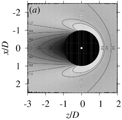
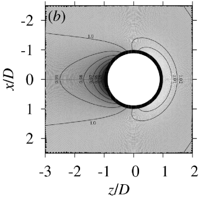
Figure 2: Contour plots of the density of ideal polymers for a flow velocity $c^{\ast}=10$. The white circle at the origin is the colloidal particle with radius $R$, the black circle is the annulus of thickness $d$ and outer diameter $D$ which is unaccessible to the polymer centers due to the hard-wall interaction, c.f. Fig. 1. $(a)$ corresponds to a uniform flow $\mathbf{u}(\mathbf{r})=-c\,\mathbf{\hat{e}}_{z}$ (i.e., to $R^{\ast}=0$). The maximum density in front of the colloid is $\rho(\mathbf{r})/\rho_{0}=6.31$. $(b)$ corresponds to $R^{\ast}=0.9$. The bow effect is reduced drastically. The maximum density in front of the colloid is $\rho(\mathbf{r})/\rho_{0}=1.05$.

As demonstrated for $R^{\ast}=0$ and $R^{\ast}=0.9$ in Figs. 2(a) and (b), respectively, the bow wave effect is large when the colloid is small compared to the polymers and does not distort too much the flow, reaching its maximum as $R^{\ast}\to 0$. This is the case investigated in Penna et al. (2003). When the colloid is large compared to the polymers, the bow wave effect is small. In the limit $d/R\to 0$, the effect vanishes completely since the polymers behave like solvent molecules. Figs. 3(a) and (b) shows the density right in front of the colloid as a function of $R^{\ast}$ and of $c^{\ast}$, respectively. The density of ideal solute particles scales almost linearly with the velocity $c^{\ast}$.

Figure 3: Density of ideal polymers at the point $x=y=0$, $z/D=1$, i.e., right in front of the forbidden zone around the colloid. (a) shows $\rho(0,0,D)$ as a function of the colloid size for $c^{\ast}=1$ and $c^{\ast}=10$. (b) shows $\rho(0,0,D)$ as a function of $c^{\ast}$ for different values of $R^{\ast}$.

III.2 Gaussian polymers

Here we address the case of interacting polymers. We consider the same polymer–polymer interaction potential studied in Ref. Penna et al. (2003), namely

$$V(r)=T\exp{[-(r/\sigma)^{2}]}.$$ (22)

The interaction of the polymers with the colloidal particle is modelled as an external potential of the form

$$U(r)=10\,T\exp{[-(r/a)^{6}]}.$$ (23)

This potential rises steeply up to $10\,T$, thus resembling a hard wall. The length $a$ must be related to the radius of the forbidden zone $D$ around the colloidal particle. We conventionally set the value of $a$ by the condition $U(D)=2\,T$, giving $a\approx 0.924\,D$. We take $\sigma=2d$ (i.e., additive mixture of polymers and colloidal particle) and $R=1.7\,\sigma$, leading to $R^{\ast}\approx 0.77$, $\sigma/D\approx 0.46$. Finally, we also considered the choice $R^{\ast}=0$, $\sigma/D\approx 0.46$, which represents a hard particle that does not distort the uniform flow ($R=0$ in Eq. (1)) in a non–additive mixture ($\sigma\neq 2d$): this was the model addressed in Ref. Penna et al. (2003).

We ran Brownian dynamics (BD) simulations of this system for two values of the flow velocity corresponding to the polymer Péclet numbers $(\sigma/D)c^{\ast}=1$ and $10$ studied in Ref. Penna et al. (2003) (i.e., $c^{\ast}\approx 2.2$ and $22$). We considered a colloidal particle at the center of a box of dimensions $L_{x}=L_{y}=12\,\sigma$ and $L_{z}=24\,\sigma$ with periodic boundary conditions. The box contained $N=3456$ polymers, corresponding to a mean polymer number density $\rho_{0}\,\sigma^{3}=1$. We took a timestep of $0.003\,\sigma^{2}\Gamma/T$ for the discretized Langevin dynamics. The system was allowed to relax for $10^{5}$ timesteps, after which collection of data was carried out during $10^{6}$ timesteps. Even though the simulated system is finite we used the analytically known flow field around a sphere in an infinite medium, Eq. (1). The error due to the truncation of this flow by the boundary of the simulation box is largest (about 20%) at the midplane of the colloid ($z=0$). This introduces effectively a discontinuity in the flow velocity field at the boundary which we discuss later.

We also solved numerically the dDFT in the random phase approximation (a mean–field model), i.e., with

$$\mathcal{F}_{\!\!\text{ex}}[\rho]=\frac{1}{2}\iint\limits_{\mathcal{V}^{2}}d^{3}r\,d^{3}r^{\prime}\;V(|\mathbf{r}-\mathbf{r}^{\prime}|)\rho(\mathbf{r})\rho(\mathbf{r}^{\prime}).$$ (24)

The time evolution given by Eq. (16) of an initially homogeneous density was solved in cylindrical coordinates on a grid spanning the domain $-120<z/\sigma<24$, $0\leq r_{\perp}/\sigma<60$, where $r_{\perp}=\sqrt{x^{2}+y^{2}}$. The grid constant was $0.0125\,\sigma$ near the colloid, i.e., for $|z|,r_{\perp}<6\,\sigma$, and $0.1\,\sigma$ in the rest of the domain. For details on the numerical procedure see Penna et al. (2003). The boundary condition at the domain border was $\rho=\rho_{0}$ also in this case we used the flow field given by Eq. (1). The error introduced here is smaller than in the BD simulations since the integration domain for the dDFT is larger than the BD simulation box.

Fig. 4 presents the density field $\bar{\rho}(z)$, spatially averaged over thin disks of radius $\sigma$ and thickness $2\,\Delta z=0.05\,\sigma$ centered at the $z$-axis, i.e.,

$$\bar{\rho}(z):=\frac{1}{\sigma^{2}\Delta z}\int\limits_{z-\Delta z}^{z+\Delta z}dz^{\prime}\int\limits_{0}^{\sigma}dr_{\perp}r_{\perp}\,\rho(r_{\perp},z^{\prime}).$$ (25)

The results of both the BD simulations and the dDFT illustrate the dramatic effect of advection by the Stokes flow (1). In particular, at the higher velocity $c^{\ast}=22$ and $R^{\ast}=0$ (uniform flow) there is a marked accumulation of polymers in front of the particle and a strong depletion behind it which are hardly observable for $R^{\ast}=0.77$. In general, the effect of the Stokes flow is to weaken the influence of the colloid on the density profile, as the polymers tend to be advected by the stream and to travel around the particle. Actually, for $c^{\ast}=2.2$ (and smaller) the deformation by the Stokes flow is so tiny that the dDFT profile $\bar{\rho}(z)$ in Fig. 4(a) is indistinguishable from the equilibrium profile (i.e., $c^{\ast}=0$).

Figure 4: Plots of $\bar{\rho}(z)$ defined in Eq. (25) as provided by the numerical solution of dDFT (lines) and as measured in BD simulations (symbols). (a) corresponds to a velocity $c^{\ast}=2.2$ and (b) to $c^{\ast}=22$. In each plot the results for both uniform flow ($R^{*}=0$) and Stokes flow ($R^{*}=0.77$) are presented.

We notice a discrepancy between the density profiles measured in the BD simulation and those calculated numerically in the dDFT. We attribute this to two finite–size effects in the simulation which have been confirmed by performing BD simulations in a smaller box at the same polymer number density ($L_{x}=L_{y}=8\,\sigma$, $L_{z}=16\,\sigma$, $N=1024$). First, the numerical solution of the dDFT for a Stokes flow with $c^{\ast}=22$ exhibits a long ($\approx 15\,\sigma$) tail of slight polymer depletion ($\rho\approx 0.98\,\rho_{0}$) behind the colloidal particle. The tail is longer than the length of the BD simulation box in $z$-direction and, as a consequence of the periodic boundary conditions, the inflowing density far ahead of the particle is smaller than $\rho_{0}$. This screening effect is very noticeable when the flow is approximated as uniform because the depletion of polymers behind the colloidal particle is very large, see Fig. 4(b). But in the case of the Stokes flow, this effect seems to less important compared to the second effect: the discontinuity of the normal component of the flow field at the lateral boundaries of the simulation box leads to a non-vanishing divergence of the flow there (we remind that the flow described by Eq. (1) has $\nabla\cdot\mathbf{u}=0$). Fig. 5 represents the density profile averaged over thin cylindrical shells of height $\sigma$ and radial thickness $\Delta r=0.05\,\sigma$ coaxial with the $z$-axis, i.e.,

$$\hat{\rho}(r_{\perp},z_{c}):=\frac{1}{\sigma\left(r_{\perp}+\frac{\Delta r}{2}\right)\Delta r}\int\limits_{z_{c}-\frac{\sigma}{2}}^{z_{c}+\frac{\sigma}{2}}\!\!dz^{\prime}\int\limits_{r_{\perp}}^{r_{\perp}+\Delta r}\!\!dr^{\prime}_{\perp}r^{\prime}_{\perp}\,\rho(r^{\prime}_{\perp},z^{\prime}).$$ (26)

The periodic boundary conditions imply that $\nabla\cdot\mathbf{u}<0$ effectively at the side boundaries located upstream, where therefore the density is enhanced: Even though we expect the density to decrease towards $\rho_{0}$ as the radial distance $r_{\perp}$ to the colloid increases we find instead an increase of the density at the boundary of the simulation box. At the side boundaries located downstream, on the other hand, $\nabla\cdot\mathbf{u}>0$ and the region near the boundary of the simulation box becomes depleted of polymers. As expected this effect is enhanced for reduced box size, see the inset in Fig. 5. The comparison of the BD results with the dDFT calculation in Fig. 4 indicates that the overall consequence of these effects is a density enhancement near the colloidal particle. In view of these important finite–size effects, we cannot quantify the validity of the approximation given by Eq. (16) for a realistic flow. When there is only uniform flow ($R^{\ast}=0$), however, the finite–size effects are much less pronounced and we find a good agreement between BD simulations and dDFT calculations, in concordance with Ref. Penna et al. (2003).

Figure 5: The plot represents $\hat{\rho}(r_{\perp},z_{c})$, see Eq. (26), in a Stokes flow ($R^{*}=0.77$) with $c^{\ast}=22$ upstream (at $z_{c}=1.5\sigma$, triangles up) and downstream (at $z_{c}=-1.5\sigma$ triangles down) of the colloid, as measured in BD simulations. The inset shows the results for a smaller simulation box.

III.3 Drag force on colloids

We have also measured the force in the $z$-direction exerted by the polymers on the particle. This force is additional to the Stokes drag force $F_{\text{Stokes}}$ exerted by the flowing solvent. If $\Gamma$ in Eq. (2) is assumed to be given by the Stokes-Einstein relation for spherical polymers of diameter $\sigma$, the Stokes drag for a colloid of radius $R$ in the same solvent is given by $F_{\text{Stokes}}=2\,c^{\ast}\,(R/\sigma)\,(T/D)$. For example, for the colloid radius $R^{\ast}=0.77$ considered in the BD simulations this gives $F_{\text{Stokes}}=3.4\,c^{\ast}\,T/D$.

In the BD simulations, the force excerted on the colloid by the polymers can be measured directly. In the case of ideal particles discussed in Sec. III.1 we use the ideal gas law $p=T\,\rho$ in order to calculate the local pressure on the colloid surface. Integrating the local pressure over the surface yields the force on the colloid.

Table 1 collects the mean force for different types of flow ($R^{\ast}=0$ for uniform flow and $R^{\ast}=0.77$ for Stokes flow) and velocities. The results confirm the necessity to take the solvent flow into account: the mean force in the case of Stokes flow is markedly smaller (at most of the order of $F_{\text{Stokes}}$) than in the case of a homogeneous flow and the dependence on $c^{\ast}$ is milder. This can be understood in terms of the reduction of the bow wave effect in the density profile around the particle by the Stokes flow in the solvent which advects the polymers. The forces in the BD simulations are of the same order of magnitude as in the ideal case, but in the case of the Stokes flow they have a weaker dependence on $c^{\ast}$.

Because the sizes involved are of the order of the microscopic length $D$, the variance of the force measured in the Brownian dynamics is relatively large. However, we find that it is not affected by the flow type and velocity and it coincides with the variance of $F_{z}$ we have measured in the equilibrium state ($c^{\ast}=0$). For comparison, Tab. 2 collects the force measured in the BD simulation in the smaller box. The increased force is consistent with the density enhancement near the particle caused by the finite–size effects. We also attribute the increase of the fluctuations to these effects.

Type of flow	$c^{\ast}$	$|\langle F_{z}\rangle|$	ideal $F_{z}$	$F_{\text{Stokes}}$
uniform	2.2	42.5	41.9
Stokes	2.2	6.38	3.14	7.48
uniform	22	215	290
Stokes	22	10.3	18.0	74.8

Table 1: Mean force exerted by the polymers measured in the BD simulations for different types of flow ($R^{\ast}=0$ for the uniform flow, and $R^{\ast}=0.77$ for the Stokes flow), compared to the force exerted by ideal polymers and to the Stokes friction of the colloid. The forces are given in units of $T/D$.

simulation box size	$c^{\ast}$	$|\langle F_{z}\rangle|$	$\sqrt{\langle F_{z}^{2}\rangle-\langle F_{z}\rangle^{2}}$
small	2.2	11	63.4
large	2.2	6.4	103
small	22	19	65.6
large	22	10	103

Table 2: Mean and variance of the force exerted by the polymers in a Stokes flow measured in BD simulations of different boxsizes (see Sec. III.2). The forces are given in units of $T/D$.

IV Conclusions

We have proposed a dynamic density functional theory (dDFT), Eq. (16), for interacting Brownian particles in a flowing solvent under the assumption that detailed balance holds (which requires, in particular, a curl-free flow). We get the same equation as already derived in Marconi and Tarazona (1999) but with the partial time derivative replaced by the total (material) time derivative. The whole effect of the flow field can be summarized into a modified external potential, allowing application of the whole machinery of equilibrium statistical mechanics. Thus, we are able to find an H-theorem for a modified free energy.

In this paper we include the displacement of the solvent by the colloid, but the hydrodynamic interactions between the colloid and the solute particles as well as the hydrodynamic interactions among the solute particles were not taken into account. While the latter is a highly non-trivial and still open problem, the first can be included in a straightforward manner by replacing the mobility $\Gamma$ by a space dependent and symmetric mobility tensor $\mathbf{\Gamma}(\mathbf{r}_{i})$ in Eqs. (2) and (4). Thereby the noise becomes multiplicative and the appropriate calculus has to be considered such that it leads to the Fokker-Planck equation (5) with $\Gamma$ replaced by $\mathbf{\Gamma}(\mathbf{r}_{i})$. Then the equilibrium distribution is not changed. For spherical particles in the vicinity of planar walls the mobility tensor can be calculated in the limit of large distances Happel and Brenner (1965). This result has been extended to surfaces with a partial slip boundary condition in Lauga and Squires (2005). Due to the translational symmetry of the system, $\mathbf{\Gamma}$ is diagonal. While the mobility perpendicular to the wall increases with distance, the distance dependence of the mobility parallel to the wall depends on the slip condition. For no-slip it increases while for total slip it decreases with the distance to the wall. The hydrodynamic interaction between two spheres has been calculated, e.g., in the Rotne-Prager approximation Jeffrey and Onishi (1984); Dhont (1997). The derivation of Eq. (16) essentially carries through with the only exception that the quotient $\mathbf{u}(\mathbf{r_{i}})/\Gamma$ in Eq. (5) has to be replaced by a field $\mathbf{\tilde{u}}(\mathbf{r}_{i})$ with $\mathbf{\Gamma}(\mathbf{r}_{i})\cdot\mathbf{\tilde{u}}(\mathbf{r_{i}})=\mathbf{u}(\mathbf{r_{i}})$. In order to absorb the flow field into a modified external potential, $\mathbf{\tilde{u}}$ (and not only $\mathbf{u}(\mathbf{r_{i}})$) has to be curl free with $\mathbf{\tilde{u}}=-\bm{\nabla}\Phi$. Instead of Eq. (16) we then get

$$\frac{\partial\rho}{\partial t}+\bm{\nabla}\cdot(\rho\,\mathbf{u})=\bm{\nabla}\cdot\left(\rho\,\mathbf{\Gamma}(\mathbf{r})\cdot\bm{\nabla}\frac{\delta\mathcal{F}[\rho]}{\delta\rho}\right).$$ (27)

In Ref. Penna et al. (2003), the polymer distribution was studied in a polymer solution flowing uniformly through a spherical particle which is hard only for the polymers. In spite of the violation of detailed balance by the boundary conditions, the comparison between simulations and the numerical solution of the proposed dDFT was good. In this paper we have considered the more realistic case of a Stokes flow (1) around the particle. The exact solution of the ideal case (no polymer–polymer interaction), the numerical solution of the interacting case as well as the corresponding Brownian dynamics simulations evidence all the dramatic effect by advection on the properties of the stationary solution. We conclude that the approximation of uniform flow, as employed in Refs. Penna et al. (2003); Dzubiella et al. (2003); Krüger and Rauscher (2007), is quantitatively bad. We have found discrepancies in the density distribution of polymers as measured in the simulations and as computed numerically in the framework of the dDFT. However, the discrepancies could be rationalized in terms of finite–size effects in the simulations due to the slow decay of the Stokes flow far from the obstacle. Thus, although a quantitative check of the validity of the approximations leading to the dDFT in Eq. (16) and of its validity for non-potential flows was not possible the results are encouraging.