Influence of deterministic trend on the estimated parameters of GARCH(1,1) model

Abstract

The log returns of financial time series are usually modeled by means of the stationary GARCH(1,1) stochastic process or its generalizations which can not properly describe the nonstationary deterministic components of the original series. We analyze the influence of deterministic trends on the GARCH(1,1) parameters using Monte Carlo simulations. The statistical ensembles contain numerically generated time series composed by GARCH(1,1) noise superposed on deterministic trends. The GARCH(1,1) parameters characteristic for financial time series longer than one year are not affected by the detrending errors. We also show that if the ARCH coefficient is greater than the GARCH coefficient, then the estimated GARCH(1,1) parameters depend on the number of monotonic parts of the trend and on the ratio between the trend and the noise amplitudes.

,

1 Introduction

The log returns of financial time series $\{P_{t}\}$ (share prices, stock indices, foreign exchange rates, etc.)

$$X_{t}=\log(P_{t}/P_{t-1})=\log\left(P_{t}\right)-\log\left(P_{t-1}\right)~{},$$ (1)

usually presents the following features: they are uncorrelated, their volatility clusters, they have fat-tailed distributions (leptokurtosis), a leverage effect is present (changes in stock prices tend to be negatively correlated with changes in volatility), their autocorrelation function decays exponentially, their absolute values present a long range dependence [2]. One of the most used stochastic models that reproduces some of these features is the Generalized Auto Regressive Conditional Heteroskedasticity (GARCH) model having the variance expressed as a linear function of past squared innovations and earlier calculated conditional variances [1]. There are various generalizations of the GARCH model, however the most used in practical applications is its simplest form, GARCH(1,1).

According to relation (1) the stationary GARCH(1,1) process is suitable for modeling time series for which $\{\log P_{t}\}$ has a linear trend, i.e. the original time series $\{P_{t}\}$ contains an exponential trend. But the nonlinear trends in $\{\log P_{t}\}$ are not eliminated by the differentiation (1). This problem is amplified in the case of a nonmonotonic trend. An alternative to the stationary modeling of financial series is the hypothesis of a nonstationary evolution. For example Stărică and Granger [5] propose a nonstationary model locally approximated by a stationary one

$$X_{t}=\mu\left(t\right)+\sigma\left(t\right)\varepsilon_{t}\ ,$$ (2)

where $\varepsilon_{t}$ are i.i.d with $E(\varepsilon_{t})=0$ and $E(\varepsilon_{t}^{2})=1$ and the unconditional mean $\mu\left(t\right)$ and the unconditional variance $\sigma\left(t\right)$ are functions of $t.$ If a nonstationary series (2) is modeled with a stationary process, then the deterministic trend $\mu(t)$ is confounded with a stochastic trend and the model tends to approach its nonstationarity limit. In the case of GARCH model this is the so called IGARCH effect.

In this paper we study the influence of a deterministic trend on the parameters of GARCH(1,1) model. We use a Monte Carlo method in order to evaluate the influence of the detrending errors on the variability of the estimated GARCH(1,1) parameters. The paper is organized as follows. In the following section we shortly present the GARCH(1,1) model and we study the intrinsic variability of its parameters. In the third section an automatic method to generate artificially trends is described. Then we present the variability of the GARCH(1,1) parameters due to the detrending of an artificially added deterministic component and the last section is dedicated to conclusions.

2 GARCH(1,1) model

The GARCH(1,1) process is a real-valued discrete time stochastic process $\{x_{t}\}$

$$x_{t}|\left\{x_{t-1},\sigma_{t-1}\right\}\sim N\left(0,\sigma_{t}^{2}\right)$$

$$\sigma_{t}^{2}=K+\alpha x_{t-1}^{2}+\beta\sigma_{t-1}^{2}$$

where $K>0,$ $\alpha\geq 0,$ $\beta\geq 0$ [1]. If $\alpha+\beta<1$, then GARCH(1,1) process is wide sense stationary with $E\left(x_{t}\right)=0,$ var$\left(x_{t}\right)=K/\left(1-\alpha-\beta\right)$ and cov$\left(x_{t},x_{s}\right)=$var$\left(x_{t}\right)\delta_{ts}$.

We analyze the daily Dow Jones Composite (DJC) series containing $N=5089$ values between 01 February 1980 and 31 December 1999 when a deterministic trend is likely to exist. The parameters of the GARCH(1,1) model obtained using the maximum likelihood method for the log returns of this series are: $\alpha_{DJ}=0.0837$, $\beta_{DJ}=0.8898$, $K_{DJ}=2.5\cdot 10^{-6}.$ With these values we have generated three index series with the same initial value on the same time interval. In Fig. 1 one observes large differences between the generated series and the initial one, especially for large $t$. This behavior is in accordance with the fact that GARCH model is suitable only for relatively short periods of time [3]. When the series length is large, then the GARCH parameters are close to the nonstationarity limit ($\alpha+\beta=1$) and the deterministic trend (if it exists) is lost or is strongly distorted because it is replaced with a stochastic one. In the case of the analyzed DJC index $\alpha_{DJ}+\beta_{DJ}=0.9735$. Therefore, the variability of the realizations of a GARCH process with given parameters is very large, especially when the series length is large.

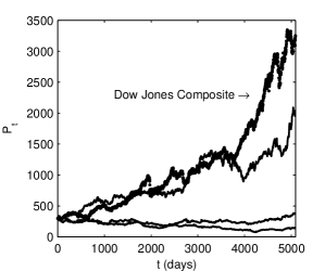
Figure 1: Dow Jones Composite index series over the period 01.02.1980-31.12.1999 and three index series simulated with GARCH(1,1) model

In order to correctly evaluate the variability of the parameters due to detrending, it must be compared with the intrinsic variability of the GARCH(1,1) parameters for time series without trends. The intrinsic variability is determined using a Monte Carlo simulation. For a given length $N$ we generate 500 realizations of a GARCH(1,1) process with the parameters ($\alpha_{DJ}$, $\beta_{DJ}$, $K_{DJ}$). For each realization the GARCH(1,1) parameters are estimated by applying the maximum likelihood method. The relative standard deviation of the GARCH(1,1) parameters decreases to an almost stationary value for large values of $N$ (Fig. 2a). Generally, the mean of the estimated parameters almost coincides with the values used for generating the series with the exception of $\beta$ (Fig. 2b). In the following we consider series with length $N=6000$ which have a variability near the stationary value.

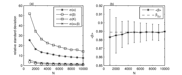
Figure 2: The relative standard deviation of the GARCH(1,1) parameters (a) and the mean of $\beta$ (b) for statistical ensembles with 500 numerically generated series with DJ parameters for each length $N$.

3 Automatically generated trends

In order to be representative, the Monte Carlo statistics must contain a large number of numerical simulations with variability comparable with those appearing in practical applications. We describe an automatic method for generating time series containing a deterministic trend which satisfies these conditions. The generation of a large number of trends with a significant variability using a fixed functional form requires a large number of parameters. For example, a polynomial trend must have a large enough degree, hence the number of its coefficients is also large. If we choose the coefficients by means of a random algorithm, then the form of the generated trend is difficult to be controlled. Usually the resulting trend has only a few parts with significant monotonic variation.

We generate a trend $\left\{f_{n}\right\}$, $n=1,2,...,N$ by joining together $s$ monotonic semiperiods of sinus with random amplitudes and lengths. In this way we obtain a large enough variability for the generated trends and we can control the number and the amplitude of its monotonic parts. We need only three parameters: the length of the series $N$ (in the following $N=6000$), the number of monotonic parts $s$ (in our tests $s=1,2,3,4$) and the minimum number of points in a part equal with 50. The amplitudes of the sinusoidal parts will be random numbers with uniform distribution $a_{p}\in\left(0,1\right)$. The value of the trend at the point $n$ of the part $p$, $N_{p}<n\leqslant N_{p+1}$, is given by the recurrence relation

$$f_{n}=f_{N_{p}}+(-1)^{p}a_{p}\left[1-\sin\frac{\pi}{2}\left(1+2\frac{n-N_{p}}{N_{p+1}-N_{p}}\right)\right]~{},$$ (3)

where $f_{1}=0$. Some trends with different values for $s$ are represented in Fig. 3.

Figure 3: Artificially generated trends with 2, 3, and 4 monotonic parts

We want to evaluate the error of the estimated GARCH(1,1) parameters due to the difference between the estimated trend and the real one. The statistical ensembles for the Monte Carlo simulations are composed by numerically generated series composed by a random component and the trend (3). First we generate a GARCH(1,1) time series $\{x_{i}\}$ with given parameters ($\alpha_{0},\beta_{0},K_{0}$). Then we calculate the series $y_{n}=\sum_{i=1}^{n}x_{i},$ (corresponding to the logarithm of a price series) and we add an automatically generated trend, $\xi_{n}=f_{n}+y_{n}$. The relation between these two components in the resulting series is characterized by the ratio $r$ of the amplitude of the trend and of the noise

$$r=\frac{\max(f_{n})-\min(f_{n})}{\max(y_{n})-\min(y_{n})}~{}.$$

If we randomly choose the number $s$ of trend parts between two given values $s_{\min}=1$ and $s_{\max}=4$ and the ratio $r$ between $r_{\min}=0.25$ and $r_{\max}=4$ we obtain a significant statistics.

From the series $\{\xi_{n}\}$ we extract a polynomial estimated trend $\{\widetilde{f}_{n}\}$, $\widetilde{y}_{n}=\xi_{n}-\widetilde{f}_{n},$ and we calculate the estimated returns $\widetilde{x}_{n}=\widetilde{y}_{n+1}-\widetilde{y}_{n}$. Then we evaluate the GARCH(1,1) parameters ($\widetilde{\alpha},\widetilde{\beta},\widetilde{K}$) using the maximum likelihood method. When we choose the degree of the polynomial estimated trend we must take into account that if it is too large, then the estimated trend begins to follow the fluctuations of the noise. From numerical tests it has resulted an optimal degree equal to $2s+3$.

4 GARCH(1,1) parameters variability due to detrending

Figure 4 shows the results obtained by applying the evaluation method of the variability of GARCH(1,1) parameters described in the previous section for statistical ensembles of 100 time series generated with the DJC parameters for different values of $r$ and $s$. From Fig. 4a it results that the averages of the estimated parameter $\widetilde{\beta}$ are randomly distributed around the initial value $\beta_{DJ}$ and they are not influenced by the number of monotonic parts of the trend $s$ or by the ratio $r.$ The other GARCH(1,1) parameters have a similar behavior so we have not represented them. Figure 4b confirms this result by means of the relative standard deviation for $s=4$. Hence, the GARCH(1,1) parameters are not influenced by detrending a nonlinear trend if the noise is generated using ($\alpha_{DJ}$, $\beta_{DJ}$, $K_{DJ}$).

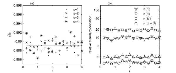
Figure 4: The variability of the GARCH(1,1) parameters due to detrending errors with respect to the ratio $r$ between the trend and the noise amplitude. The statistical ensembles contain 100 generated GARCH(1,1) series with the DJC parameters superposed on automatically generated trends. (a) The average value of the estimated $\widetilde{\beta}$ for different numbers of trend monotonic parts. The continuous line corresponds to the value $\beta_{DJ}=0.8898$ used to generate the GARCH(1,1) noise. (b) The relative standard deviation of the GARCH(1,1) parameters for the generated noise $x_{n}$ (continuous line) and for the estimated noise $\widetilde{x}_{n}$ (markers) for $s=4$.

In our case the coefficient $\beta_{DJ}=0.8898$ has a much greater value than $\alpha_{DJ}=0.083$. The variability of the GARCH(1,1) parameters at detrending for greater ratios $\alpha_{0}/\beta_{0}$ is presented in Fig. 5. The number of parts of the artificially generated trend is $s=4$ and the ratio between trend and noise is $r=2$ and $\alpha_{0}$ and $\beta_{0}$ are varied such that $\alpha_{0}+\beta_{0}$ remains constant, $\alpha_{0}+\beta_{0}=0.972$ and $K_{0}=K_{DJ}$. One observes that for $\beta_{0}\geq 0.7$ the mean of the estimated values $\left\langle\widetilde{\beta}\right\rangle$ almost coincides with the initial value $\beta_{0}$ and the relative standard deviation is less than 3%. Hence, the behavior observed for DJC index is the same for smaller values of $\beta_{0}.\$But the error $\left\langle\widetilde{\beta}\right\rangle-\beta_{0}$ and the relative standard deviation $\sigma\left(\widetilde{\beta}\right)$ significantly increases when $\beta$ decreases below $0.6$, so in this cases the influence of the errors of the estimated trend is significant. The other two GARCH(1,1) parameters have a similar behavior.

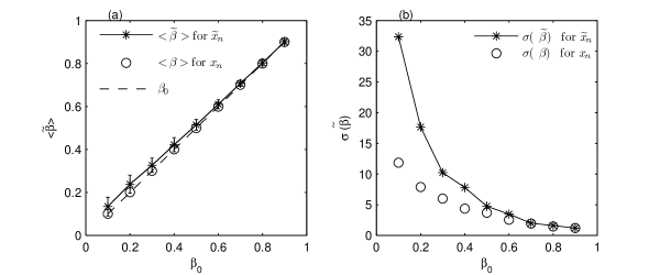
Figure 5: The variability of the parameter $\widetilde{\beta}$ due to the detrending error for statistical ensembles of 100 generated GARCH(1,1) series with the DJ parameters superposed on automatically generated trends for $s=4$, $r=2$ and $\alpha_{0}+\beta_{0}=0.972$. (a) The dashed line corresponds to the values $\beta_{0}$ used to generate the GARCH(1,1) noise.

Hence the influence of detrending on the variability of GARCH(1,1) parameters is due especially to the coefficient $\beta$ that generalizes the ARCH model. Figure 6 contains the results of a detailed analysis for the minimum value $\beta_{0}=0.1$ in Fig. 5. The variability of the estimated GARCH(1,1) parameters significantly increases when the number $s$ of monotonic parts of the trend increases and the ratio $r$ between the variation amplitude of the trend and the noise is larger.

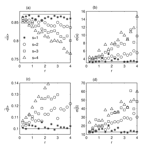
Figure 6: The mean and relative standard deviation of the GARCH(1,1) parameters estimated for $\widetilde{x}_{n}$ obtained on statistical ensembles of 100 time series for each $r$ and $s$. The continuous line in (a) represents $\alpha_{0}$, in (c) $\beta_{0}$, in (b) represents $\sigma(\alpha)$ and in (d) $\sigma(\beta)$.

5 Conclusions

An important problem in the analysis of financial series is to separate the deterministic component and the stochastic one. In this paper we have analyzed the influence of the nonstationarity due to a deterministic trend on the GARCH(1,1) model and we have shown that for long periods of tens of years the results obtained with this model are not sensitive to the existence of a nonlinear trend. This behavior occurs for large values of the GARCH parameter $\beta$ and $\alpha+\beta$ close to 1. But for small values of $\beta$  and large values of $\alpha$ such that $\alpha+\beta\simeq 1$ the influence of detrending on the GARCH(1,1) model becomes significant.

References

- [1] Bollereslev T., Journal of Econometrics 31 (1986) 307.
- [2] R.N. Mantegna, H.E. Stanley, An Introduction to Econophysics, Correlations and Complexity in Finance, Cambridge University Press, Cambridge, 2000.
- [3] Th. Mikosch, C. Stărică, Is it really long memory we see in financial returns?, in Extremes and Integrated Management, Ed. P. Embrechts, Risk Books, UBS Warburg, 2000.
- [4] C. Stărică, Is GARCH(1,1) as good a model as the Nobel prize accolades would imply?, Preprint, Chalmers University of Technology, Gothenburg, 2003.
- [5] C. Stărică, C. Granger, The Review of Economics and Statistics 87 (2005) 503.