The effect of the motion of the Sun on the light-time in interplanetary relativity experiments

Abstract

In 2002 a measurement of the effect of solar gravity upon the phase of coherent microwave beams passing near the Sun has been carried out with the Cassini mission, allowing a very accurate measurement of the PPN parameter $\gamma$. The data have been analyzed with NASA’s Orbit Determination Program (ODP) in the Barycentric Celestial Reference System, in which the Sun moves around the centre of mass of the solar system with a velocity $v_{\odot}$ of about 10 m/sec; the question arises, what correction this implies for the predicted phase shift. After a review of the way the ODP works, we set the problem in the framework of Lorentz (and Galilean) transformations and evaluate the correction; it is several orders of magnitude below our experimental accuracy. We also discuss a recent paper [10], which claims wrong and much larger corrections, and clarify the reasons for the discrepancy.

1 Introduction

In 2002 the Cassini spacecraft, on its cruise to Saturn, has allowed an outstanding measurement of the effect of solar gravity on the phase of a coherent microwave beam sent from the ground antenna to the on-board transponder and transmitted back. The data have been analysed with the Orbit Determination Program (ODP), a numerical code developed at NASA’s Jet Propulsion Laboratory for accurate space navigation, including relativistic effects; its algorithms are described in detail in [14] (referred to here as the Manual). In the rest frame of the Sun the total phase change can be measured by the light-time $t_{2}-t_{1}$ between the events 1 and 2, the start and the arrival of a photon in the up- or the down-link, respectively:

$$t_{2}-t_{1}=r_{12}+\Delta t=r_{12}+(\gamma+1)m\ln\frac{r_{1}+r_{2}+r_{12}}{r_{1}+r_{2}-r_{12}}.$$ (1)

Here $r_{1}$ and $r_{2}$ are the distances of 1 and 2 from the Sun at their appropriate times $t_{1}$ and $t_{2}$; $r_{12}$ is their Euclidian distance; $m=1.43$ km is the gravitational radius of the Sun. This formula shows a characteristic enhancement in the delay $\Delta t$ near conjunction, when the impact parameter $b$ of the ray is much smaller than both $r_{1}$ and $r_{2}$; in this case the argument of the logarithm in (1) is about $4r_{1}r_{2}/b^{2}$, as in eq. (1) of [4]. This approximation, however, is not accurate enough and is never used in the ODP. The fractional change in frequency $\Delta y$ is essentially the rate of change of the light-time; as one can intuitively see, and as fully discussed in [3] (quoted as BG), this frequency shift is of order $\alpha v$, where $\alpha$ is the deflection angle and $v$ a linear combination of the velocities of the end points. The fit of the Cassini data gave the result:

$$\gamma-1=(2.1\pm 2.3)\times 10^{-5}.$$ (2)

An important feature of the experiment was the use of a multi-frequency link, which allowed an excellent elimination of the contribution of the plasma in the solar corona. To date, this is by far the best measurement of the PPN parameter $\gamma$, which has a crucial role in discriminating between alternative theories of gravity.

Due to the other planets, in particular Jupiter, the Sun moves around the centre of gravity of the solar system with a velocity $v_{\odot}\approx 5\times 10^{-8}$ (15 m/sec) and a time scale of several years. During a light-time (about an hour) its motion is essentially uniform, so that its effect on the light-time can be described by a Lorentz transformation and has nothing to do with the intrinsic scattering dynamics. The short Nature paper [4] does not mention the motion of the Sun. The Manual does not address this problem explicitly, nor evaluate the correction; however, we show that the ODP does take into account this effect, and the fractional correction to the one-way gravitational delay $\Delta t$ is of order $v_{\odot}$, quite below the experimental sensitivity. The effect can also be described in terms of the induced fractional frequency shift $\Delta y=\alpha v$, which attained the value $3\times 10^{-10}$ in the best passage. We show that the motion of the Sun causes a change in $\Delta y$ of order $\alpha vv_{\odot}$, much smaller than the frequency noise $\sigma_{y}\approx 10^{-14}$. In a two-way experiment, like Cassini’s, even this small correction largely cancels out. In Sec. 4 we discuss the recent paper [10], which claims wrong and much larger corrections, and point out the reasons for the discrepancy. Einstein’s prediction $\gamma=1$ is still unchallenged.

2 Using the Orbit Determination Program

The theoretical discussion in the main text of [4] (eqs. (1) and (2)) was given only to help physical understanding. The Block 5 receivers at the ground station count the cycles of the phase of the received coherent beam relative to the local frequency standard and determine the number of cycles in successive time intervals. The duration of these intervals can be chosen from 0.1 sec to several hours (Sec. 13.3.1.3 of the Manual); during Cassini’s experiment it was 1 sec, but further averaging was done in the analysis. The extraction of a time derivative from the actual phase count, which contains fast-varying components, would be very delicate; the frequency is never measured, nor is needed, since the mathematical expression of the predicted light-time is at hand. This is why the ODP deals only with light-time. The difference between Cassini’s experiment and measurements of the radar delay does not lie in a different gravitational observable, but in the fact that Cassini uses a coherent radio beam and its phase as the main observable, while planetary radar determines the arrival time of a wave packet through the peak of its intensity. The strongest useful signal in Cassini’s experiment occurred on day 2 after conjunction, when the logarithm in (1) was about 10, with a delay

$$\Delta t=1.43\,(\gamma+1)\,10^{6}\,\mathrm{cm};$$

thus the formal accuracy $2.3\times 10^{-5}$ in $\gamma$ corresponds to an accuracy of 30 cm in $\Delta t$.

The ODP includes a very extensive and well tested orbit determination program, with which the orbits $\mathbf{r}_{i}(t)$ of the centres of all relevant bodies in the solar system, including the Sun and any spacecraft, are determined numerically from previous and current observations. Following standard astronomical usage and IAU recommendations, in particular the 2000 IAU resolutions, this is carried out in the solar system Barycentric Celestial Reference System (BCRS). The excellent paper [22] (referred here as S) describes the procedure in detail. The expression S(8) for the metric tensor is the basis for the definition of this frame; but, as T. Damour has discussed in the first [6] of four papers on relativistic frames, strictly speaking the BCRS cannot be described in a single coordinate chart, but must use a global chart for the dynamics of the gravitating bodies, and a local chart for each gravitating body. In the linearized approximation we use, however, this is not needed and S(8) has a global meaning. In the BCRS the origin is at the centre of gravity C of the solar system; its axes are anchored to the non rotating ‘celestial sphere’ – the International Celestial Reference System (ICRS) – as realized by very distant astronomical sources. Harmonic coordinates are used: to the required order, gravity is described by a (‘small’) spacetime tensor $h_{\mu\nu}$ in a fixed and conventional Minkowsky background with metric $\eta_{\mu\nu}=\mathrm{diag}(-1,1,1,1)$. In this view one can use Lorentz formalism; the word ‘null’, the proper time $\tau$ and raising and lowering spacetime indices refer to this metric. In addition, the (cartesian) space components $h_{mn}$ are proportional to the unit matrix $\delta_{mn}$ (the coordinates are ‘isotropic’). The time coordinate is the Barycentric Coordinate Time (TCB), related to the Earth-bound Geocentric Coordinate Time (TCG) by eq. S(58), in which, essentially, the Doppler shifts due to the motion of the Earth and the gravitational shift due to external gravitating bodies are corrected for.

In the present paper we only need to consider, besides the BCRS, the heliocentric reference frame, neglecting quadratic terms in its gravitational potential and the contributions of other masses. Then in isotropic coordinates both $h_{00}$ and the space components $h_{mn}$ are functions only of the distance $R$ from the origin. Note that in general relativity the field equations do not uniquely determine the metric tensor in terms of the radial coordinate; in our special coordinates this gauge freedom is forfeited. The time coordinate $T$ is the privileged and invariant Killing time, with respect to which the metric tensor is constant. The standard textbook expression for the light-time (see, e.g., [25]) reads

$$T_{2}-T_{1}=R_{12}+\Delta T=R_{12}+(\gamma+1)m\ln\frac{R_{1}+R_{2}+R_{12}}{R_{1}+R_{2}-R_{12}}.$$ (3)

The coordinates of the end events are $x_{1}^{\mu}=(T_{1},\mathbf{R}_{1}),\>x_{2}^{\mu}=(T_{2},\mathbf{R}_{2})$. It should be noted that this formula holds only in isotropic coordinates.

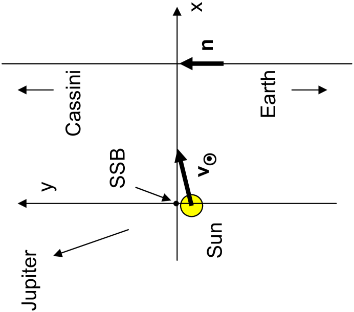
Figure 1: The geometry of the experiment in the BCRS frame at epoch June 23-th 2002 20:00:00 UT, the first useful passage after conjunction in the Cassini experiment. The center of the Sun moves in the ecliptic plane around the barycenter of the solar system (SSB) in a roughly circular orbit with radius $7.8\times 10^{8}$m; its velocity $v_{\odot}=14.6$ m/sec is approximately orthogonal to the direction of Jupiter, and the orbital period is $\approx 12$ y.

The ODP instead (see Fig. 1) computes the light-time in the BCRS, where the centre of the Sun $\mathbf{r}_{\odot}(t)$ moves around C with a velocity $v_{\odot}\approx 3\times 10^{-8}$; squares of $v_{\odot}$ can be neglected. As described in Sec. 8.3.6 of the Manual, a special subroutine implements the formula (1) in 32 steps, an inclusion discussed at length in [8]. The main object of the present paper is to evaluate the difference in the light-time in the two frames.

In the Manual, Sec. 8.3.1.1, the three quantities $r_{1}$, $r_{2}$ and $r_{12}$ are defined in barycentric coordinates as follows. The numerical code provides for the bodies 1 and 2 and for the Sun the orbits $\mathbf{r}_{1}^{C}(t)$, $\mathbf{r}_{2}^{C}(t)$, $\mathbf{r}_{\odot}^{C}(t)$ relative to C in the BCRS. The simultaneous differences (eq. (8-62) of the Manual)

$$\mathbf{r}_{1}(t_{1})=\mathbf{r}_{1}^{C}(t_{1})-\mathbf{r}_{\odot}^{C}(t_{1}),\quad\mathbf{r}_{2}(t_{2})=\mathbf{r}_{2}^{C}(t_{2})-\mathbf{r}_{\odot}^{C}(t_{2})$$ (4)

provide $r_{1}=|\mathbf{r}_{1}(t_{1})|$ and $r_{2}=|\mathbf{r}_{2}(t_{2})|$; $r_{12}$ is the modulus of

$$\mathbf{r}_{12}=\mathbf{r}_{2}(t_{2})-\mathbf{r}_{1}(t_{1}).$$ (5)

Note that differences between positions of bodies taken at the same time are invariant under Galilei transformations; hence $r_{1}$, $r_{2}$ and $r_{12}$ have, up to $O(v_{\odot}^{2})$, the same value in the rest frame and the barycentric frame. We’ll return to this important point later.

It is useful to clarify the logical status of eq. (1) and of the subroutine used in the ODP to implement it, as explained in Sec. 8.3.2 of the Manual. Given the arrival time $t_{2}$ at the point $\mathbf{r}_{2}(t_{2})$, the light-time solution must provide the starting time $t_{1}$, and the position and velocity of the transmitter 1 at that time. A first approximation to $t_{1}$ is given by the geometrical solution

$$t_{1}=t_{2}-r_{12}(t_{1}),$$

where the argument of the distance indicates the time at which 1 is taken; an error $\Delta t\approx 10^{-4}$ sec is made due to the neglected gravitational delay. In this short time interval the velocity of 1 is uniform and a linear correction $\delta t_{1}$

$$t_{1}+\delta t_{1}=t_{2}-r_{12}(t_{1})-\delta t_{1}\frac{dr_{12}}{dt_{1}}-\Delta t$$

is sufficient. The corrected value of the light-time is then compared with the observations.

3 Measuring the light-time in the barycentric frame

We first comment about coordinates and geometrical objects. In the ODP scheme – the radial coordinate $r$ being fixed – physical laws and statements are invariant under the Lorentz group; to deal with this requirement we take the geometric point of view, in which scalars, vectors and tensors – like $h_{\mu\nu}$ – denote a geometrical object, independent of its coordinate representation. Measured quantities are invariant scalars. The choice of coordinates is conventional and free; for a vector, like $v_{\mu}=(v_{0},\textbf{v})$, they are indicated in round brackets, with the space components in bold type.

We only need to deal with the spacetime vector $\ell^{\mu}$ from 1 to 2, the geometric object which summarizes the scattering dynamics of the experiment. In the rest frame, where the Sun sits at the origin, its components are

$$\ell^{\mu}=x_{2}^{\mu}-x_{1}^{\mu}=(T_{2}-T_{1},\mathbf{R}_{12})=(R_{12}+\Delta T,\mathbf{R}_{2}-\mathbf{R}_{1});$$ (6)

if the mass $m$ vanishes

$$\ell^{\mu}=(R_{12},\mathbf{R}_{12})$$

is null; gravity just adds a small, time-like and positive contribution $(\Delta T,\mathbf{0})$ along the time coordinate. An observer with (constant) spacetime velocity vector $v^{\mu}$ measures the light-time $-v_{\mu}\ell^{\mu}$; if the observer is at rest relative to the Sun, $v^{\mu}_{\odot}=(1,\mathbf{0})$ and the previous result $T_{2}-T_{1}$ is recovered; if it is at rest relative to the barycenter C, the ODP value $t_{2}-t_{1}$ is obtained. Of course, the components of the light-time in the two systems are related by a Lorentz transformation.

[10], [9] and other papers take a different approach. They apply the appropriate Lorentz transformation to the full trajectory of the photon in the rest frame (as given, for instance, in [25]) and obtain its expression in the barycentric frame; then they compute the elapsed time. Delay and bending of the transformed orbit are then determined by the gravity of a moving Sun, with new gravitomagnetic terms appearing. This complicates matters. A similar situation would arise in the classical Rutherford scattering of an electron by a proton, normally described by the Coulomb field of the latter, assumed at rest; of course, one would get the same result in a frame where the proton moves, provided the magnetic field so generated is taken into account. Just as magnetism is the direct consequence of the fact that under Lorentz transformations the electromagnetic potential behaves as a four-vector, so gravitomagnetic metric perturbations arise due to Lorentz invariance and the tensorial character of the metric.

The analysis of Cassini’s experiment has been carried out in the standard framework of a Lorentz invariant theory. If Lorentz invariance is violated, gravitomagnetism does not have the standard form; moreover, the problem of the effect of the motion of the Sun on the gravitational delay must be addressed in a way different from the one we follow below. KPSV suggest that, with its excellent accuracy, Cassini’s experiment may set better limits to such violations. This would require a wise decision about the best theoretical scheme and the appropriate parametrization; besides the PPN preferred frame formalism, one has vector-tensor theories (see [25]) and Lorentz-violating electromagnetism, on which there is a wide literature (see [15], [16], [18], [1]). Current limits from other experiments should also be taken into account. This program is outside the present paper.

It is more convenient to skip the formal coordinate change in the trajectory and to use just the light-time vector – a geometrical object – expressed as

$$\ell^{\mu}=(t_{2}-t_{1},\mathbf{x}_{2}-\mathbf{x}_{1})$$

in the barycentric frame and as

$$\ell^{\mu}=(T_{2}-T_{1},\mathbf{R}_{2}-\mathbf{R}_{1})$$

in the rest frame of the Sun. The barycentric components are related to (6) by a Lorentz transformation corresponding to the (small) velocity of the Sun $\mathbf{v}_{\odot}$:

$$t_{2}-t_{1} = T_{2}-T_{1}+\mathbf{v}_{\odot}\cdot\mathbf{R}_{12}+O(v_{\odot}^{2}),$$ (7)

$$\mathbf{x}_{2}-\mathbf{x}_{1} = \mathbf{R}_{12}+\mathbf{v}_{\odot}(T_{2}-T_{1})+O(v_{\odot}^{2}).$$ (8)

The space part is just a Galilei transformation, arising from the fact that the end events occur at different times. In Galileian relativity time is invariant; but this holds only if the space component of a vector upon which the transformation operates is much smaller than the time component. In our case $\ell^{\mu}$ is almost null and (7) must be taken into account. The transformation conserves proper length to the appropriate approximation:

$$(t_{2}-t_{1})^{2}-|\mathbf{x}_{2}-\mathbf{x}_{1}|^{2}=(T_{2}-T_{1})^{2}-R_{12}^{2}+O(v_{\odot}^{2});$$ (9)

or, neglecting squares of the delay,

$$\Delta t\,|\mathbf{x}_{2}-\mathbf{x}_{1}|=\Delta TR_{12}.$$ (10)

Now

$$\mathbf{x}_{2}-\mathbf{x}_{1}=\mathbf{r}_{2}^{C}(t_{2})-\mathbf{r}_{1}^{C}(t_{1}),$$

the space component of $\ell^{\mu}$ in barycentric coordinates, obviously is not Galilei invariant; but the Manual shrewdly uses $\mathbf{r}_{12}$ instead, which, being built with simultaneous vectors, almost compensates the Galilei transformation (8). Indeed, from (5)

$$\mathbf{r}_{12}=\mathbf{x}_{2}-\mathbf{x}_{1}-\mathbf{v}_{\odot}(t_{2}-t_{1});$$ (11)

comparing it with (8), we see that

$$\mathbf{r}_{12}-\mathbf{R}_{12}=O(v_{\odot}^{2}).$$

Let $\mathbf{n}=\mathbf{r}_{12}/r_{12}$ be the (Galilei invariant!) unit vector along the unpertubed ray from 1 to 2, as computed in the Manual. Eq. (8) gives, to $O(v_{\odot}^{2})$,

$$|\mathbf{x}_{2}-\mathbf{x}_{1}|=R_{12}+\mathbf{v}_{\odot}\cdot\mathbf{n}(T_{2}-T_{1}),$$

so that

$$\Delta t=\Delta T(1-\mathbf{v}_{\odot}\cdot\mathbf{n}),$$ (12)

which is our final result. It corresponds to a negligible change of about a millimiter in light-time. On p. 8-28 the Manual acknowledges the neglect of this correction: The error in the calculated delay due to ignoring the barycentric velocity $v_{\odot}$ of the gravitating body has an order of magnitude equal to the calculated delay multiplied by the velocity of the body/$c$. Our procedure clearly shows the gist of the problem, how the delay transforms under a Lorentz transformation with a small velocity. As C. M. Will has pointed out to us, a simpler proof is based upon his eq. (7.3) in [25], which says how the perturbation in the coordinate of the photon along the ray changes with time; in the barycentric frame (7.3) acquires an additional term due to the time-space components of the metric and proportional to $m/r$; this leads to our result. Note also that in a two-way experiment, like Cassini’s, in the down-link $\mathbf{n}$ is almost equal and opposite its up-link value and the two contributions essentially cancel out; a net result arises from second order terms $O(v_{\odot}^{2})$ in the Lorentz transformation.

Eq. (12) does not say, however, how to evaluate the delay in terms of the distances $r_{1},r_{2}$ and $r_{12}$ obtained in the BCRS. We need their expressions in a generic frame, such that they reduce to $R_{1}$, $R_{2}$ and $R_{12}$ in the rest frame. In the present context, invariance under the approximate Lorentz group (7) and (8) is sufficient. Then the ODP expressions (4) and (5) provide the straightforward answer: in fact they are constructed with simultaneous differences and (8) reduces to Galilei transformations.

It interesting to discuss the fully invariant case. Distances arise here because the Sun affects a photon essentially through the scalar potential $U$, the fundamental solution of D’Alembert’s equation. In the rest frame and, say, for a photon at the start event $x_{1}^{\mu}=(T_{1},\mathbf{R}_{1})$,

$$U=\frac{m}{|\mathbf{R}_{1}|}=\frac{m}{R_{1}}.$$ (13)

We want to express it in a generic frame, with the Sun moving with an arbitrary (but constant) four-velocity $v_{\odot}^{\mu}=dX^{\mu}/d\tau$. The cartesian distance $R_{1}$ must be replaced with the unique quantity which (i) is Lorentz invariant and (ii) reduces to $R_{1}$ when $v_{\odot\mu}=(-1,\mathbf{0})$ (the minus sign being required by the metric $\mathrm{diag}(-1,1,1,1)$). This is a textbook problem in electrodynamics (e. g., see [11], Sec. 63). Let $X^{\mu}_{1}$ be the (ante-dated) intersection of the (straight) world-line of the Sun with the past light-cone of the start event $x_{1}^{\mu}=X_{1}^{\mu}+\ell_{1}^{\mu}$; $\ell_{1}^{\mu}$ is the corresponding, future-pointing null vector. The required ‘distance’ is the invariant

$$r_{1}^{\star}=\left|v_{\odot\mu}(x_{1}^{\mu}-X^{\mu}_{1})\right|=\left|v_{\odot\mu}\ell_{1}^{\mu}\right|.$$ (14)

Indeed, since

$$x_{1}^{0}-X^{0}_{1}=|\mathbf{x}_{1}-\mathbf{X}_{1}|$$

(elapsed time is equal to distance), it obviously fulfils (ii). The future light-cone would give the same result.

In the appropriate slow motion approximation $v_{\odot\mu}=(-1,\mathbf{v}_{\odot})$ and (14) reads

$$r_{1}^{\star}=x_{1}^{0}-X_{1}^{0}-\mathbf{v}_{\odot}\cdot(\mathbf{x}_{1}-\mathbf{X}_{1})+O(v_{\odot})^{2}.$$ (15)

$x_{1}^{0}-X_{1}^{0}$, the antedated distance between the event 1 and the Sun, differs from the simultaneous value by an amount equal to the distance traveled by the Sun in a time equal to the distance itself; hence $r_{1}^{\star}$ is, to $O(v_{\odot})$, just the simultaneous distance $r_{1}$ (see (4) used in the ODP. In other words, the first-order correction to Lienard-Wiechert potential due to a slowly moving source vanishes.

The fully invariant form of $r_{12}=|\mathbf{r}_{2}-\mathbf{r}_{1}|$ is

$$r_{12}^{\star}=|v_{\odot\mu}\ell^{\mu}|=|v_{\odot\mu}(x_{2}^{\mu}-x_{1}^{\mu})|;$$ (16)

indeed, in the rest frame $x_{1}^{\mu}=(T_{1},\mathbf{R}_{1})$ and $x_{1}^{\mu}=(T_{2},\mathbf{R}_{2})$, with $T_{2}-T_{1}=|\mathbf{R}_{2}-\mathbf{R}_{1}|=R_{12}$. We now show that in the slow motion approximation

$$r_{12}^{\star}=x_{2}^{0}-x_{1}^{0}-\mathbf{v}_{\odot}\cdot(\mathbf{x}_{2}-\mathbf{x}_{1})+O(v_{\odot})^{2}$$ (17)

reduces to modulus of the ODP (5). We must use the simultaneous relative vector $\mathbf{r}_{1}=\mathbf{x}_{1}-\mathbf{X}(x_{1}^{0})$, which differs from the space part of $\ell_{1}^{\mu}$

$$\mbox{\boldmath$\ell_{1}$}=\mathbf{x}_{1}-\mathbf{X}_{1}=\mathbf{x}_{1}-\mathbf{X}(x_{1}^{0}-r_{1})=\mathbf{r}_{1}+r_{1}\mathbf{v}_{\odot}$$

because of the ante-dated time argument in the position $\mathbf{X}(x^{0})$ of the Sun. With a similar first-order expansion we get

$$\mathbf{X}_{2}-\mathbf{X}_{1}=\mathbf{X}(x_{2}^{0}-r_{2})-\mathbf{X}(x_{1}^{0}-r_{1})=(x_{2}^{0}-x_{1}^{0}-r_{2}+r_{1})\mathbf{v}_{\odot}=(r_{12}-r_{2}+r_{1})\mathbf{v}_{\odot},$$

where we have used

$$\mathbf{X}(x^{0}_{2})-\mathbf{X}(x^{0}_{1})=\mathbf{v}_{\odot}(x_{2}^{0}-x_{1}^{0}),$$

$x_{2}^{0}-x_{1}^{0}=|\mathbf{x}_{2}-\mathbf{x}_{1}|$ and the fact that $\mathbf{x}_{2}-\mathbf{x}_{1}$ differs from $\mathbf{r}_{2}-\mathbf{r}_{1}=\mathbf{r}_{12}$ by $O(v_{\odot})^{2}$. Then

$$r_{12}^{\star} = |\mathbf{x}_{2}-\mathbf{x}_{1}|-\mathbf{r}_{12}\cdot\mathbf{v}_{\odot}=|\mathbf{r}_{12}+\mathbf{X}_{2}-\mathbf{X}_{1}+(r_{2}-r_{1})\mathbf{v}_{\odot}|-\mathbf{r}_{12}\cdot\mathbf{v}_{\odot}=$$

$$= |\mathbf{r}_{12}+r_{12}\mathbf{v}_{\odot}|-\mathbf{r}_{12}\cdot\mathbf{v}_{\odot}=r_{12}+O(v_{\odot})^{2}.$$

We see that the ODP variable $r_{12}$ is the appropriate approximation of a fully invariant quantity and describes correctly the gravitational interaction.

4 About Galilei invariance

KPSV make two different claims about the effect of the motion of the Sun. Their expression of the gravitational delay in the barycentric frame KPSV(25)

$$\Delta_{{}_{K}}t=(\gamma+1)m\ln\frac{r_{1}+r_{2}+r-\mathbf{r}\cdot\mathbf{v}_{\odot}}{r_{1}+r_{2}-r+\mathbf{r}\cdot\mathbf{v}_{\odot}}.$$ (18)

differs from our analysis in two ways. First, it is based upon the coordinate transformation KPSV(11), which does not provide the required, first order difference between $t$ and $T$ (eq. (7)); this makes it impossible to get the true correction (12). More important, the quantity $r_{12}$ used in the ODP is not their $r$, which, in our notation, is $|\mathbf{x}_{2}-\mathbf{x}_{1}|$. This quantity is not a Galilei invariant and cannot appear in the argument of the logarithm. This argument must depend on the coordinates of the photon relative to the Sun. Let us see the consequences of this claim. In the extreme conjunction case ($b\ll(r_{1},r_{2}))$ the correction in the denominator of the argument of the logarithm prevails and (18) reads

$$\Delta_{{}_{K}}t=(\gamma+1)m\left(\ln\frac{4r_{1}r_{2}}{b^{2}}-\mathbf{v}_{\odot}\cdot\mathbf{n}\frac{r_{1}r_{2}}{b^{2}}\right).$$

The claimed correction $\approx mv_{\odot}$ is similar to the true correction (12), but is enhanced when $b$ is small.

In their second claim, KPSV consider the description of the experiment in terms of the effect that the deflection has on the frequencies recorded by two very distant clocks (see [3]). Of course the deflection angle

$$\alpha=2(\gamma+1)\frac{m}{b}$$ (19)

is meaningful only in the extreme conjunction approximation $b\ll(r_{1},r_{2})$, which we assume here for the sake of illustration. This gives also, in order of magnitude, the change in the angle between the velocity $\mathbf{V}$ of a far-away clock relative to the Sun and the beam, and corresponds to a (one-way) fractional frequency change (for a grazing ray and the Earth’s orbital velocity) of order

$$\Delta y\approx\alpha V\approx 8\times 10^{-10}.$$ (20)

Explicitly (see eq. (22) of BG), in the rest frame we have

$$\Delta y=\frac{(\mathbf{V}_{2}\cdot\hat{\mathbf{b}})r_{1}-(\mathbf{V}_{1}\cdot\hat{\mathbf{b}})r_{2}}{r_{12}}\>\frac{2(\gamma+1)m}{b}.$$ (21)

In the following, for simplicity, we only consider frequency measurements in terms of the proper times of 1 and 2. Now $\Delta y$, a ratio of proper frequencies, is a Lorentz-invariant scalar; to get its expression in a slowly moving frame, note first that the time coordinate is not involved, so that only Galilei transformations need to be considered. We just need the unique quantity which (i) is Galilei invariant and (ii) reduces to (21) in the rest frame. The impact parameter vector is the component of $\mathbf{r}_{2}$ (or, equivalently, $-\mathbf{r}_{1}$) along the ray:

$$\mathbf{b}=\mathbf{r}_{2}-(\mathbf{n}\cdot\mathbf{r}_{2})\mathbf{n}.$$ (22)

This is invariant. Secondly, and trivially, the rest-frame vectors $\mathbf{V}_{1}$ and $\mathbf{V}_{2}$ should be replaced with their invariant forms

$$\mathbf{v}_{1}-\mathbf{v}_{\odot}=\frac{d\mathbf{r}_{1}(t_{1})}{dt},\quad\mathbf{v}_{2}-\mathbf{v}_{\odot}=\frac{d\mathbf{r}_{2}(t_{2})}{dt}.$$ (23)

KPSV claim that in the barycentric frame, due to the motion of the Sun, there is an additional correction

$$\Delta_{K}y\approx\alpha v_{\odot}\approx 3\times 10^{-13}.$$ (24)

The fact that the impact parameter vector (parallel to the deflection vector $\alpha$) is a Galilei invariant seems to be ignored; it is defined in the rest frame in terms of absolute coordinates, with no reference to the Sun. Then in the barycentric frame the correction KPSV(18) arises, which produces a small correction $O(v_{\odot})$ in the frequency shift. Moreover, absolute velocities are used in the analogue of (21), which, after a Galilei transformation, produces KPSV(21), the basis for their main claim. Of course, the claimed correction (24) is absorbed in (21) using the relative velocities $\mathbf{v}_{1}-\mathbf{v}_{\odot},\mathbf{v}_{2}-\mathbf{v}_{\odot}$.

In Cassini’s experiment the standard deviation of the residual frequency noise (at an integration time of 1000 sec; see Fig. S2 of the supplementary material of [4]) was $\sigma_{y}=0.7\times 10^{-14}$. While the magnitude of the correction (24) stated by KPSV is 40 times larger, the paper does not even suggest a violation of general relativity. In the experiment $N=1094$ data points, obtained after several pre-processing steps, have been used, with a remarkably Gaussian distribution of the frequency residuals, as impressively shown by Fig. 3 of [4]. The sensitivity of $\gamma$ from each data point is difficult to ascertain, but surely the final error in $\gamma$ which results from the fit is smaller than $\sigma_{y}$. KPSV, instead, state the opposite (top of p. 280) and thereby avoid dangerous conclusions. In our view, if the ODP dynamical model were as inaccurate as claimed by KPSV, the inescapable conclusion would be that the good orbital fit and the agreement with the standard prediction are the result of an exceedingly unlikely chance; accepting the KPSV correction would imply the first experimental violation of general relativity.

5 Conclusion

Cassini’s experiment, by far the most accurate attempt to measure the PPN parameters, did not pose a threat to Einstein’s theory of gravitation, nor answer the major question, at what level and how it is violated. The measurement of the deflection parameter $\gamma$ has a crucial importance; although no theoretical prediction is at hand about its deviation from unity, alternative theories based upon a long range scalar field require $\gamma<1$. In the future steady improvements in instrumentation, in particular space astrometry and the use of optical links in interplanetary space, will allow much more accurate measurements, and new relativistic space missions are under construction or in the planning phase; see [24] and [21] for reviews. We quote, in particular, the astrometric mission GAIA [12], the experimental program MORE [13] in the BepiColombo mission to Mercury and the project LATOR [23]. Optical interferometric measurements, similar to those under development for gravitational wave detection (the LISA project), are planned for the ASTROD mission ([17], [19], [20]). Binary pulsars, whose gravitational field is much stronger, will also play a role in testing gravitational theories.

A numerical code for relativistic orbit determination more accurate than the ODP is surely needed. Aside from the correction (12) in the light-time, terms in the metric quadratic in the gravitational radius $m$ must be included. The second order gravitational deflection depends on the radial gauge (see [5]); in the isotropic gauge, for a grazing ray, it has the value $\alpha_{\mathrm{quad}}=1.2\times 10^{-11}$, corresponding to a frequency shift $\approx v_{\odot}\alpha_{\mathrm{quad}}=10^{-15}$, an accuracy easily accessible with laboratory standards. We should also mention that in conjunction experiments, besides the obvious smallness parameter $m/R_{\odot}=2\times 10^{-6}$, the smallness of $b/r$ may produce an enhancement in the light-time. At the first order in $m$ this is already apparent in the logarithmic term of (1); but there is also a quadratic correction to the light-time of order $mr/b^{2}$, which may produce an effect in Cassini’s experiment about the same as the formal error. A correction of this kind is included in the ODP. Finally, the complex procedures used in the definition and the construction of the BCRS and the TCB need to be revisited and improved both at the fundamental level and in the numerical implementation.

References

References

- [1] Bailey Q G and Kostelecky V A 2006 Signals for Lorentz violation in post-Newtonian gravity Phys. Rev. D 74 045001
- [2] Bertotti B, Farinella P and Vokrouhlický D 2003 Physics of the solar system (Dordrecht: Kluwer)
- [3] Bertotti B and Giampieri G 1992 Relativistic effects for Doppler measurements near solar conjunction Class. Quantum Grav. 9 777-793. Quoted as BG
- [4] Bertotti B Iess L and Tortora P 2003 A test of general relativity using radio links with the Cassini spacecraft Nature 425 374-376
- [5] Bodenner J and Will C M 2003 Deflection of light to second order: a tool for illustrating principles of general relativity Am. J. Phys. 71 770-773
- [6] Damour T, Soffel M and Xu C 1991 General relativistic celestial mechanics. I. Method and definition of reference systems Phys. Rev. D 43 3273-3307
- [7] Eddington A 1960 The mathematical theory of relativity Cambridge: Cambridge University Press
- [8] Hellings R W 1986 Relativistic effects in astronomical time measurements A. J. 91 650-659
- [9] Klioner S 2003 Light propagation in the gravitational field of moving bodies by means of Lorentz transformations. I. Mass monopoles moving with constant velocities Astron. Astrophys. 404 783-787
- [10] Kopeikin S M, Polnarev A G, Schäfer G and Vlasov I Yu 2007 Gravimagnetic effect of the barycentric motion of the Sun and determination of the post-Newtonian parameter in the Cassini experiment Phys. Lett. A, 367 276-280. Quoted as KPSV in the text.
- [11] Landau L D and Lifshitz E M 1975 The classical theory of fields Oxford: Butterworth and Heinemann
- [12] Mignard F 2001 Fundamental physics with GAIA J. Phys. IV France 1 1-12
- [13] Milani A, Vokrouhlický D, Villani D et al 2002 Testing general relativity with the BepiColombo radio science experiment Phys. Rev. D 66 1-21
- [14] Moyer T D 2003 Formulation for observed and computed values of Deep Space Network data types for navigation, (Hoboken, New Jersey: Wiley). Called Manual
- [15] Ni W-T 1977 Equivalence Principle and electromagnetism Phys. Rev. 38 301-303
- [16] Ni W-T 1984 Equivalence principles and precision experiments in: Precision Measurement and Fundamental Constants II (B N Taylor and W D Phillips, eds) National Bureau of Standards Special Publication No. 617, (U.S. Government Printing Office, Washington D.C., US) 647-651
- [17] Ni W-T, Shiomi S and Liao A-C 2004 ASTROD, ASTROD I and their gravitational-wave sensitivities Class. Quantum Grav. 21 S641-S646
- [18] Ni W-T 2005 Empirical foundations of relativistic gravity Int. J. Mod. Phys. D14 901-921
- [19] Ni W-T, Bao Y, Dittus H et al 2006 ASTROD I: mission concept and Venus flyby Acta Astronautica 59 598-607
- [20] Ni W-T 2007 ASTROD (Astrodynamical space test of relativity using optical devices) and ASTROD I Nuclear Physics B (Proc. Suppl.) 166, 153-158
- [21] Ni W-T, Paton A P and Xia Y, 2008 Testing relativistic gravity to one part per billion, in: Lasers, clocks and drag-free control (H Dittus, C L mmerzahl and S G Turyshev, eds) Astrophysics and Space Science Library, 349
- [22] Soffel M, Klioner S A, Petit G ey al 2003 The IAU 2000 resolutions for astrometry, celestial mechanics and metrology in the relativistic framework: explanatory supplement A. J. 126 2687-2706. Quoted as S
- [23] Turyshev S G, Shao M and Nordtvedt K 2004 The laser astrometric test of relativity mission Class. Quantum Grav. 21 2773-2779
- [24] Turyshev S G, Shao M and Nordtvedt K 2008, in: H Dittus, C Lämmerzahl and S G Turyshev Lasers, clocks and drag-free: exploration of relativistic gravity in space. Berlin: Springer 429-493
- [25] Will C M 1993 Theory and experiment in gravitational physics Cambridge: Cambridge University Press