Analysis of stochastic fluid queues driven by local time processes

Abstract

We consider a stochastic fluid queue served by a constant rate server and driven by a process which is the local time of a certain Markov process. Such a stochastic system can be used as a model in a priority service system, especially when the time scales involved are fast. The input (local time) in our model is always singular with respect to the Lebesgue measure which in many applications is “close” to reality. We first discuss how to rigorously construct the (necessarily) unique stationary version of the system under some natural stability conditions. We then consider the distribution of performance steady-state characteristics, namely, the buffer content, the idle period and the busy period. These derivations are much based on the fact that the inverse of the local time of a Markov process is a Lévy process (a subordinator) hence making the theory of Lévy processes applicable. Another important ingredient in our approach is the Palm calculus coming from the point process point of view.

Keywords: Local time, fluid queue, Lévy process, Skorokhod reflection, performance analysis, Palm calculus, inspection paradox.

AMS Classification: 60G10, 60G50, 60G51, 90B15.

1 Introduction

This paper extends the results of Mannersalo et al. [13] who introduced a fluid queue (or storage process) driven by the local time at zero of a reflected Brownian motion and served by a deterministic server with constant rate. The motivation provided in [13] is that the system provides a macroscopic view of a priority queue with two priority classes. Indeed, in such a system, the highest priority class (class 1) goes through as if the lowest one does not exist, whereas the lowest priority class (class 2) gets served whenever no item of the highest priority is present. In telecommunications terminology, class 2 only receives whatever bandwidth remains after class 1 served. As argued in [13], if the highest priority queue is, macroscopically, approximated by a reflected Brownian motion, the lowest priority queue is driven by the cumulative idle time of the first one, which is approximated by the local time of the reflected Brownian motion at $0$.

In view of Internet networking applications, such as the service provision amongst several classes of service (e.g. streaming video and expedited data), the fluid or macroscopic model is thus quite appropriate for obtaining a better picture of the situation and for performance analysis and design. From a mathematical point of view, the model is a rare example of a non-trivial fluid queue whose performance characteristics (such as steady-distribution) can be computed explicitly. If, in addition, we take into account the heavy-tailed nature of traffic on the Internet, it seems reasonable to consider a Lévy process as a model for class 1 queue. This provides motivation for studying a queue whose input is the local time of a reflected Lévy process.

More generally, let $X$ be a Markov process and $L$ its local time at a specific point. The fluid queue driven by $X$ refers to the stochastic system defined by

$$Q_{t}=Q_{0}+L_{t}-t+I_{t},\quad t\geq 0,$$

where $Q_{t}\geq 0$ for all $t\geq 0$, and $I$ is a non-decreasing process, starting from $0$, such that

$$\int_{0}^{\infty}{\text{\Large$\mathfrak{1}$}}(Q_{s}>0)dI_{s}=0.$$

Thus, $Q$ is obtained by Skorokhod reflection and $I$ is necessarily given by

$$I_{t}=-\inf_{0\leq s\leq t}[(Q_{0}+L_{s}-s)\wedge 0];$$

see [8]. By considering, instead of $0$, an arbitrary initial time, we can define a proper stochastic dynamical system (see Appendix A for details) which, under natural conditions, admits a unique stationary version. To this we refer frequently throughout the paper.

We remark also that in Kozlova and Salminen [10] the situation in which $X$ is a general one-dimensional diffusion is analysed. Moreover, Sirviö (née Kozlova) [16] studies the case where $L$ is constructed as the inverse of a general subordinator (without specialising the underlying process $X$).

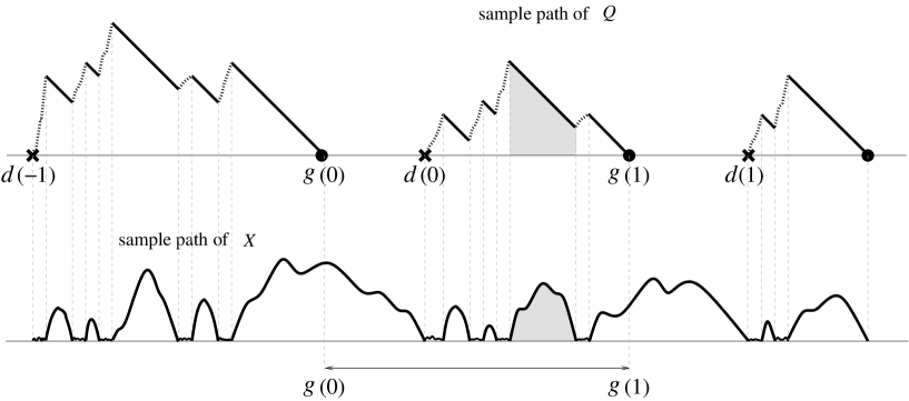
Figure 1: Typical behaviour of $Q$ and the background Markov process $X$ when the underlying Lévy process $Y$ has unbounded variation paths. By convention, the origin of time is contained between $g(0)$ and $d(0)$. Note that excursions of $X$ away from $0$ correspond to intervals over which $Q$ decreases.

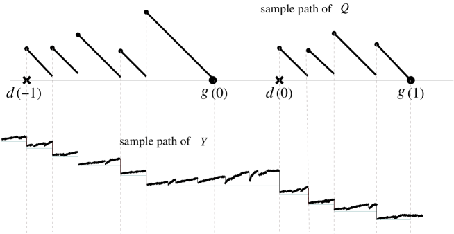
Figure 2: Typical behaviour of $Q$ and the background Lévy process $Y$, in case that $Y$ is spectrally negative with bounded variation paths.

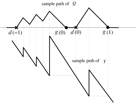
Figure 3: Typical behaviour of $Q$ and the background Lévy process $Y$, in case that $Y$ is spectrally positive with bounded variation paths. Here, only the case where the jump part of $Y$ is compound Poisson is depicted. When $Q_{t}>0$ and $X_{t}=0$, we see that $Q_{t}$ increases at rate $|d_{Y}|-1$, where $d_{Y}<-1$ is the drift of $Y$.

This paper follows ideas which were developed in [16] in the context of reflection of the inverse of a subordinator. However, (1) it connects the abstract framework with the case where the subordinator is the local time of a reflected Lévy process (motivated by applications in priority processing systems) (2) it uses, as much as possible, a framework based on Palm probabilities (see, in particular, Section 4–Theorem 3 and Section 5–Lemma 2), and (3) explicitly discusses the possible types of sample path behaviour of the process of interest ($Q$); for illustration, see Figures 1, 2 and 3: Figure 1 concerns the case where $Q$ has continuous sample paths but with parts which are singular with respect to the Lebesgue measure. Figure 2 concerns the case where $Q$ has paths with isolated discontinuities (positive jumps) and linear decrease between them. Figure 3 concerns the case where $Q$ has absolutely continuous paths. The cases are exhaustive. Despite the wide variety of sample paths (depending on the type of underlying Lévy process $Y$), the mathematical framework and formulae derived have a uniform appearance.

The paper is organised as follows. In Section 2 we construct the stationary version of the underlying (background) Markov process $X$. In Section 3 we construct the stationary version of stochastic fluid queue with input the local time of $X$, based on the stationary version of $X$. In Section 4 we derive the stationary distribution of the buffer content and present a number of examples. In Section 5 we examine the idle and busy periods, and, in particular, characterise the distributions of their starting and ending times. The analysis is carried out first under the condition that the time at which the system is observed is a typical point of and idle or a busy period. Finally, the distributions of typical idle and busy periods are derived.

2 The background Markov process and its local time

We first construct the underlying Markov process $X$ which models the highest priority class. This process will be taken to be the stationary reflection of a spectrally one-sided Lévy process

$$Y=(Y_{t},~{}t\in\mathbb{R})$$

with two-sided time and $Y_{0}=0$ (see Appendix B). A Lévy process is called spectrally negative if its Lévy measure $\Pi$ satisfies

$$\Pi((-\infty,0))>0\quad{\rm and}\quad\Pi((0,+\infty))=0,$$

and spectrally positive if

$$\Pi((-\infty,0))=0\quad{\rm and}\quad\Pi((0,+\infty))>0.$$

Clearly, if $Y$ is spectrally positive then $-Y$ is spectrally negative, and vice versa. To avoid trivialities we shall throughout assume that

$$|Y|$$ does not have monotone paths

which rules out the cases that $Y$ is an increasing or decreasing subordinator.

We also discuss the characteristics of its local time at $0$. Appendix A summarises the notation and results on the Skorokhod reflection problem and its stationary solution. Appendix B summarises some facts on Lévy processes with one sided jumps indexed by $\mathbb{R}$. We will throughout denote by $P$ a probability measure which is invariant under time shifts, and by $P_{x}$ the conditional probability measure when $X_{0}=x$. We define the Laplace exponent of a spectrally one-sided Lévy process as a function $\psi_{Y}:\mathbb{R}_{+}\to\mathbb{R}$ given for $\theta\geq 0$ by

$$\psi_{Y}(\theta):=\begin{cases}\log Ee^{\theta(Y_{t+1}-Y_{t})},&\text{ if $Y$ is spectrally negative },\\ \log Ee^{-\theta(Y_{t+1}-Y_{t})},&\text{ if $Y$ is spectrally positive}.\end{cases}$$

Thus we insist that $\psi_{Y}$ be defined on $\mathbb{R}_{+}$, and define its right inverse

$$\Phi_{Y}(q):=\sup\{\theta\geq 0:~{}\psi_{Y}(\theta)=q\},\quad q\geq 0.$$ (1)

We use also the notation

$$\overline{Y}_{t}:=\sup_{0\leq s\leq t}Y_{s}\quad{\rm and}\quad\underline{Y}_{t}:=\inf_{0\leq s\leq t}Y_{s},\quad t\geq 0,$$

and recall the duality lemma for Lévy processes (see, e.g., Bertoin [2, p. 45]):

$$\{Y_{t}-Y_{(t-s)-}\,:\,0\leq s\leq t\}\stackrel{{\scriptstyle\text{\rm d}}}{{=}}\{Y_{s}\,:\,0\leq s\leq t\},$$ (2)

where $\stackrel{{\scriptstyle\text{\rm d}}}{{=}}$ means equality in distribution. Hence,

$$\sup_{0\leq s\leq t}\left(Y_{t}-Y_{(t-s)-}\right)\stackrel{{\scriptstyle\text{\rm d}}}{{=}}\overline{Y}_{t},$$

which is equivalent with

$$Y_{t}-\underline{Y}_{t}\stackrel{{\scriptstyle\text{\rm d}}}{{=}}\overline{Y}_{t}.$$ (3)

In this paper, we will mainly study the Lévy process $Y$ with the time parameter taking values in the whole of $\mathbb{R}$ (see Appendix B). The Skorokhod reflection mapping associated with $\{Y_{t}\,:\,t\in\mathbb{R}\}$ is defined (see Lemma 8 in Appendix A) via

$$X_{t}:=\widetilde{\mathcal{R}}_{t}Y:=\sup_{-\infty<s\leq t}(Y_{t}-Y_{s}),\quad t\in\mathbb{R}.$$

In the remaining of this section we give conditions for the existence of the stationary process $\widetilde{\mathcal{R}}Y=(\widetilde{\mathcal{R}}_{t}Y,t\in\mathbb{R})$, compute its marginal distribution, and define the local time process $L$ of $\widetilde{\mathcal{R}}Y$ at 0 which will be used for the construction of the fluid queue. A few words about the definition of $L$ are in order. We adopt the point of view the $L$ is a stationary random measure on $(\mathbb{R},\mathscr{B})$, i.e.

$$L(s,s+t]=L(0,t]\raisebox{0.43057pt}{\scriptsize$\circ$}\theta_{s},\quad t\geq 0,\quad s\in\mathbb{R},$$

where $\theta_{s}$ is the shift on the canonical space (see Appendix B), which regenerates together with $X$ at each point $t$ at which $X_{t}=0$. It is known that $L$ is a.s. continuous if and only if the point $x=0$ is regular for the closed interval $(-\infty,0]$ for the process $X$, and this is equivalent to $\inf\{t>0:~{}Y_{t}\leq 0\}=0$, $P_{0}$-a.s. Furthermore, $L$ is a.s. absolutely continuous if and only if, in addition to the above, the point $x=0$ is irregular for the open interval $(0,\infty)$ for the process $X$, and this is equivalent to $\inf\{t>0:~{}Y_{t}>0\}>0$, $P_{0}$-a.s. If $L$ is a.s. continuous then it is not difficult to attach a physical meaning to it as a cumulative input process to a secondary queue. For mathematical completeness, we shall also consider the case where $L$ is a.s. discontinuous, in which case it can be shown to have a discrete support. In the continuous case, $L$ can be defined uniquely module a multiplicative constant. We shall make the normalization precise later. In the discontinuous case, there is more freedom; however, insisting that its inverse be a subordinator, we are left with only one choice. The discontinuous case appears only once below and the construction of $L$ is discussed there. In all cases, the support of the measure $L$ is the closure of the set $\{t\in\mathbb{R}:X_{t}=0\}$.

Associated to the measure $(L(B),B\in\mathscr{B})$ we can define a cumulative local time process, denoted (abusing notation), by the same letter, and given by:

$$L_{t}:=\begin{cases}L(0,t],&t\geq 0,\\ -L(t,0],&t<0.\end{cases}$$

The right-continuous inverse process is

$$L^{-1}_{x}:=\begin{cases}\inf\{t>0:~{}L(0,t]>x\},&x\geq 0\\ \sup\{t<0:~{}L(t,0]<x\},&x<0.\end{cases}$$ (4)

In case $L$ is $P$-a.s. continuous, the process $(L^{-1}_{x},x\in\mathbb{R})$ has, under $P_{0}$, independent increments and a.s. increasing paths (i.e. it is a, possibly killed, subordinator). This is an additional requirement that needs to be imposed when $L$ is not $P$-a.s. continuous.

Throughout the paper, we denote by $P_{x}$ the probability $P$, conditional on $X_{0}=x$.

2.1 Stationary reflection of a spectrally negative Lévy process

Suppose that the process $Y$ is a spectrally negative Lévy process with non-monotone paths; see expression (53).

Proposition 1.

Let $Y=\{Y_{t}\,:\,t\in\mathbb{R}\}$ be a spectrally negative Lévy process with two-sided time. Assume that its Laplace exponent $\psi_{Y}(\theta)=\log Ee^{\theta Y_{1}}$, $\theta>0$, is such that $\psi_{Y}^{\prime}(0+)<0$. Then

$$X=\{X_{t}:=\widetilde{\mathcal{R}}_{t}Y\,:\,t\in\mathbb{R}\}$$

is the unique stationary solution of SDS (the Skorokhod dynamical system, see Appendix A) driven by $Y$. The marginal distribution of $X$ is exponential with mean $1/\Phi_{Y}(0).$

Proof.

Since $E[Y_{t+1}-Y_{t}]=\psi^{\prime}_{Y}(0+)<0$, existence and uniqueness of the stationary solution is guaranteed by Corollary 2 of Appendix A. That $\Phi_{Y}(0)>0$ is a direct consequence of the definition of $\Phi_{Y}$ (see (1)). To derive the marginal distribution of $X$ consider for $\beta\geq 0$

$$E[e^{-\beta X_{0}}]=\lim_{t\to\infty}E_{0}[e^{-\beta(Y_{t}-\underline{Y}_{t})}]=\lim_{t\to\infty}E_{0}[e^{-\beta\overline{Y}_{t}}]$$

Since $Y$ is spectrally negative its over all supremum, $\sup_{s\geq 0}Y_{s},$ is exponentially distributed with mean $1/\Phi_{Y}(0)$ (see, e.g., Bertoin [2, p. 190] p. 190 or Kyprianou [11, p. 85]). ∎

In view of Proposition 1, we assume that

$$\psi^{\prime}_{Y}(0+)\in[-\infty,0),$$

which is equivalent to

$$\Phi_{Y}(0)>0.$$

It is easily seen that, for a non-monotone spectrally negative $Y$, a necessary and sufficient condition for continuity of $L$ is that $Y$ has unbounded variation paths. This is further equivalent to: $\sigma>0$ or $\int_{-1}^{0}|y|\Pi(dy)=\infty$.

In the alternative case, when the paths of $Y$ are of bounded variation, the number of visits of $Y$ to its running infimum forms a discrete set. So $n(s,t]:=\sum_{u\in\mathbb{R}}{\text{\Large$\mathfrak{1}$}}(X_{u}=0)$ is finite for all $-\infty<s<t<\infty$. Let $n_{t}:=n(0,t]$ if $t\geq 0$, and $n_{t}:=-n(t,0]$ if $t<0$, and let $(\mathfrak{e}_{j},j\in\mathbb{Z})$ be a collection of i.i.d. exponentials with mean $1$, independent of $Y$. We adopt the following construction for $L$.

$$L(s,t]=\sum_{n_{s}<i\leq n_{t}}\mathfrak{e}_{i},\quad-\infty<s\leq t<\infty.$$

In both cases, the process $(L^{-1}_{x},x\in\mathbb{R})$ is a subordinator under $P_{0}$, with $L^{-1}_{0}=0$, $P_{0}$-a.s. If $L$ is continuous, this property is immediate from the definition of $L$. If $L$ is discontinuous, $L^{-1}$ has independent increments due to our choice of the exponential jumps of $L$. Since $\psi^{\prime}_{Y}(0+)<0$, we have $Y_{t}\to\mp\infty$, as $t\to\pm\infty$, $P$-a.s., and this implies that $L_{t}\to\pm\infty$, as $t\to\pm\infty$, $P$-a.s. Thus, it is not possible for $L_{x}^{-1}$ to explode for finite $x$.

Regardless of the continuity of the paths of $L$, we always have the following:

Proposition 2.

Let $Y$ and $X$ be as in Proposition 1 and $L$ the local time at $0$ of $X.$Then the local time $L$ can be normalized to satisfy

$$E_{0}\big{[}e^{-qL^{-1}_{x}}\big{]}=e^{-xq/\Phi_{Y}(q)},\quad q\geq 0,$$ (5)

and, moreover,

$$E_{0}L_{x}^{-1}=x/{\Phi_{Y}(0)},\quad x\in\mathbb{R},\qquad EL_{t}=t\,\Phi_{Y}(0),\quad t\in\mathbb{R}.$$ (6)

Proof.

For the Laplace exponent of $L^{-1}_{x}$ in (5), we refer to Bingham [3, p. 731] (a result due to Fristedt [5]) and Kyprianou [11] and Kyprianou and Palmowski [12]: The “ladder process” $(L_{x}^{-1},X_{L_{x}^{-1}}),x\geq 0)$ is a Lévy process with values in $\mathbb{R}^{2}_{+}$ and Laplace exponent

$$\widehat{\kappa}(\alpha,\beta)=\log E_{0}\big{[}e^{-\alpha L_{1}^{-1}-\beta X_{L_{1}^{-1}}}\big{]}=\frac{\alpha-\psi_{Y}(\beta)}{\Phi_{Y}(\alpha)-\beta}$$

obtained by Wiener-Hopf factorisation for a spectrally negative process; see Bertoin [2, p. 191, Thm. 4]. Setting $\beta=0$ we obtain $E_{0}[e^{-\alpha L_{1}^{-1}}]=e^{-\alpha/\Phi_{Y}(\alpha)}$, as claimed. From this, we obtain $E_{0}L_{x}^{-1}=x/\Phi_{Y}(0)$, by differentiation. Using the strong law of large numbers, we have $\lim_{x\to\infty}L^{-1}_{x}/x=1/\Phi_{Y}(0)$, $P_{0}$-a.s., and, given that $(L^{-1}_{x},x>0)$ is the right-continuous inverse function of $(L_{t},t>0)$–see (4), we have $\lim_{t\to\infty}L_{t}/t=\Phi_{Y}(0)$, $P_{0}$-a.s., and $P$-a.s. Since $L$ is a stationary random measure, we have $EL_{t}=C\,t$ for some constant $C.$ Hence, we immediately have that $C=\Phi_{Y}(0)$, and this proves (6). ∎

We shall later need the $P$-distribution of the random variable

$$D:=\inf\{t>0:\,X_{t}=0\}.$$ (7)

Since $X_{0}$ is exponential with rate $\Phi_{Y}(0)$, we have $P(X_{0}>0)=1$. So if $0\leq t<D$, we have $X_{t}=X_{0}+Y_{t}$, $P$-a.s. Therefore

$$D=\inf\{t>0:~{}Y_{t}<-X_{0}\},\quad P-\text{a.s.}$$

Let

$$\tau_{-x}:=\inf\{t>0:Y_{t}<-x\}.$$

Therefore,

$$E[e^{-\theta D}] = \int_{0}^{\infty}P(X_{0}\in dx)\,E[e^{-\theta\tau_{-x}}]$$ (8)

$$= \int_{0}^{\infty}\Phi_{Y}(0)\,e^{-\Phi_{Y}(0)x}\,\left(Z^{(\theta)}(x)-\frac{\theta}{\Phi_{Y}(\theta)}W^{(\theta)}(x)\right)\,dx$$

$$= \Phi_{Y}(0)\,\frac{\psi_{Y}(\Phi_{Y}(0))\Phi_{Y}(\theta)-\theta\Phi_{Y}(0)}{\Phi_{Y}(\theta)~{}\Phi_{Y}(0)~{}[\psi_{Y}(\Phi_{Y}(0))-\theta]}$$

$$= \frac{\Phi_{Y}(0)}{\Phi_{Y}(\theta)},$$

where the overshoot formula (61) given in the Appendix B (see also Bingham [3, p. 732]) and the Laplace transforms (56), (57), for the scale functions $W^{(\theta)}$, $Z^{(\theta)}$, were used.

2.2 Stationary reflection of a spectrally positive Lévy process

We can repeat the construction in the subsection above for a spectrally positive Lévy process $Y$ with non-monotone paths. We shall be using the formulae of Appendix B with $-Y$ in place of $Y$.

Proposition 3.

Let $Y=\{Y_{t}\,:\,t\in\mathbb{R}\}$ be a spectrally positive Lévy process with two sided time and Laplace exponent $\psi_{Y}$. Assume that its Laplace exponent $\psi_{Y}(\theta)=\log Ee^{-\theta Y_{1}}$ is such that $\psi_{Y}^{\prime}(0+)>0$. Then the process $\{X_{t}:=\widetilde{\mathcal{R}}_{t}Y\,:\,t\in\mathbb{R}\}$ is the unique stationary solution to the SDS driven by $Y$. The stationary distribution of $X$ is given for $\beta\geq 0$ by

$$E[e^{-\beta X_{0}}]=\lim_{t\to\infty}E_{0}[e^{-\beta(Y_{t}-\underline{Y}_{t})}]=\lim_{t\to\infty}E_{0}[e^{-\beta\overline{Y}_{t})}]$$

$$\hskip 46.94687pt=\psi_{Y}^{\prime}(0+)\frac{\beta}{\psi_{Y}(\beta)}.$$ (9)

Proof.

Notice that in this case, by the assumption on $\psi_{Y},$

$$E[Y_{t+1}-Y_{t}]=-\psi^{\prime}_{Y}(0+)<0,$$

and, hence, $Y$ drifts to $-\infty.$ Let $Z:=-Y.$ Clearly, $Z$ is spectrally negative,

$$X_{t}=Y_{t}-\underline{Y}_{t}=\overline{Z}_{t}-Z_{t},$$

and $Z$ drifts to $+\infty.$ The classical result due to Zolotarev [18] (see also Bingham [3] Proposition 5 p. 725) says that the stationary distribution of $X$ is as given in (3). ∎

We shall therefore assume that

$$\psi^{\prime}_{Y}(0+)\in(0,\infty).$$

Hence $\Phi_{Y}=\psi_{Y}^{-1}$ and so

$$\Phi_{Y}^{\prime}(0+)=1/\psi_{Y}^{\prime}(0+)\in(0,\infty).$$

It is easily seen that, starting from $0$, the process $Y$ hits $(-\infty,0]$ immediately, $P$-a.s., and this ensures continuity of the local time $L$. Moreover, we may and do normalize $L$ so that

$$L(s,t]=-\inf_{s<u\leq t}Y(s,u].$$ (10)

The continuity of $L$ implies that

$$\{L_{x}^{-1}\,:\,x\geq 0\}=\{\tau_{-x}\,:\,x\geq 0\},$$ (11)

where $\tau_{-x}:=\inf\{t>0:Y_{t}<-x\}=\inf\{t>0:Z_{t}>x\}.$ Note that $(L_{x}^{-1},x\in\mathbb{R})$ is a subordinator under $P_{0}$, with $L^{-1}_{0}=0$, $P_{0}$-a.s. Furthermore, since $Y_{t}$ drifts to $\mp\infty$ as $t\to\pm\infty$, $L^{-1}$ is proper (not killed).

Let us briefly comment on the special case where, starting from $X_{0}=0$, the interval $(0,\infty)$ will be first visited by $X$ at an a.s. positive time. It is known [2, Ch. 7] that this occurs if and only if $Y$ has bounded variation, i.e.

$$Y(s,t]=d_{Y}(t-s)+\int_{(s,t]}\int_{(0,\infty)}y~{}\eta(du,dy),$$ (12)

where $d_{Y}$ is the drift, and $\int_{0}^{1}y~{}\Pi(dy)<\infty$. Since we exclude the case where $Y$ is monotone, we must have $d_{Y}<0$. In that case, with (10) as the definition of $L$, it is known that for all $s\leq t$,

$$L(s,t]=|d_{Y}|\int_{s}^{t}{\text{\Large$\mathfrak{1}$}}(X_{u}=0)du.$$ (13)

A rewording of the first part of Lemma 10 in Appendix B gives the first part of the following proposition.

Proposition 4.

Let $Y$ be as in Proposition 3 and $L$ the local time at $0$ of $X.$ Then

$$E_{0}[e^{-qL_{x}^{-1}}]=e^{-\Phi_{Y}(q)x},\quad q\geq 0.$$ (14)

Moreover,

$$E_{0}L_{x}^{-1}=x\Phi_{Y}^{\prime}(0+),\quad x\geq 0,\qquad EL_{t}=t\,\psi_{Y}^{\prime}(0+),\quad t\geq 0.$$ (15)

Proof.

Formula (14) follows from (11) and the well known characterisation of the distribution of the first hitting time $\tau^{+}_{x},$ see, e.g., Bingham [3] p. 720. By differentiating (14), we obtain the first part of (15), and using an ergodic argument–as in the proof of the second part of (6)–we obtain the second part of (15). ∎

We now compute the $P$-distribution of $D=\inf\{t>0:~{}X_{t}=0\}$, by arguing as earlier: we have $D=\inf\{t>0:-Y_{t}>X_{0}\}$, and, since $-Y$ is spectrally negative, we use the hitting time formula (60) of Appendix B to obtain

$$E[e^{-\theta D}]=E[e^{-\Phi_{Y}(\theta)X_{0}}]=\psi_{Y}^{\prime}(0+)~{}\frac{\Phi_{Y}(\theta)}{\psi_{Y}(\Phi_{Y}(\theta))}=\psi_{Y}^{\prime}(0+)~{}\frac{\Phi_{Y}(\theta)}{\theta},$$ (16)

where we also used (3) and the fact that $\Phi_{Y}\raisebox{0.43057pt}{\scriptsize$\circ$}\psi_{Y}$ is the identity.

3 Construction of (the stationary version of) the fluid queue with local time input

We wish to construct a fluid queue driven by

$$\widehat{L}(s,t]=L(s,t]-(t-s),$$

where $L$ is the local time at zero of the Markov process $X$. The process $X$ is a stationary Markov process which is the reflection of a spectrally negative (Section 2.1) or a spectrally positive (Section 2.2) Lévy process. In either case, $L$ is a stationary random measure with rate (see (6) and (15))

$$\mu=EL(s,s+1]=\begin{cases}\Phi_{Y}(0),&\text{ if $Y$ is spectrally negative}\\ \psi_{Y}^{\prime}(0+),&\text{ if $Y$ is spectrally positive}\end{cases}.$$ (17)

The fluid queue started from level $x$ at time $0$ is, as explained in Appendix A, the process

$$(\mathcal{R}_{0,t}\widehat{L}(x),~{}t\geq 0).$$

From Corollary 2 in Appendix A we immediately have:

Theorem 1.

If $\mu<1$ there is a unique stationary version of the fluid queue driven by $\widehat{L}$ and is given by

$$Q_{t}=\widetilde{\mathcal{R}}_{t}\widehat{L}=\sup_{-\infty<u\leq t}(\widehat{L}_{t}-\widehat{L}_{u}),\quad t\in\mathbb{R}.$$ (18)

Thus, the following assumptions will be made throughout the paper:

[A1] $\mu<1$

[A2] In case $Y$ is spectrally positive and of bounded variation then $d_{Y}<-1$

Assumption [A1] is so that we can construct a stationary version of $Q$ (as in Theorem 1). If $Y$ is spectrally positive and of bounded variation non-monotone paths then its drift $d_{Y}$ must be negative. If, however, $|d_{Y}|\leq 1$ then–see (13)–$L(s,t]\leq t-s$ for all $s<t$ and so $Q$ will be identically equal to $0$.

Physically, we think of $Q$ a stationary fluid queue whose cumulative input between times $s$ and $t$ is $L(s,t]$ and whose maximum potential output is $t-s$. Unlike $X$, the process $Q$ is not Markovian. However, since $Q$ has been built on the probability space supporting $X$, it makes sense to consider, for each $x\geq 0$, the probability measure $P_{x}$ defined as $P$ conditional on $\{X_{0}=x\}$.

Since $L$ is a random measure allows us to consider the Palm distribution with respect to it, namely the probability measure defined by

$$P_{L}(A)=\mu^{-1}E\int_{(0,1]}{\text{\Large$\mathfrak{1}$}}_{A}\raisebox{0.43057pt}{\scriptsize$\circ$}\theta_{t}L(dt).$$

Since $P_{L}$ is also given as the value of the Radon-Nikodým derivative

$$P_{L}(A)=\mu^{-1}\frac{E{\text{\Large$\mathfrak{1}$}}_{A}L(dt)}{dt}\bigg{|}_{t=0}$$

it follows that $P_{L}$ expresses conditioning with respect to the event that $t=0$ is a point of increase of $L$. But $L$ is the local time of $X$ at zero. Therefore, the support of $L$ is the set of zeros of $X$. We thus have

Theorem 2.

The Palm measure $P_{L}$ coincides with $P_{0}$.

This observation allows us to use the formulae of Appendix A involving Palm probabilities.

4 Stationary distribution of the fluid queue

We are interested in computing $P(Q_{t}\in\cdot)$, a probability measure which is the same for all $t$. We will use three properties of $L$. First, duality, i.e. that $Y$ has the same distribution when time is reversed, see (2), implies that

$$(L(0,t],~{}t\geq 0)\stackrel{{\scriptstyle\text{\rm d}}}{{=}}(L[t,0),~{}t\leq 0),\quad\text{ under $P$ and under $P_{L}$}.$$

Second, the process

$$L^{-1}_{x}=\inf\{t\geq 0:L(0,t]>x\},\quad x\geq 0$$

is a subordinator under $P_{0}$. Third, the Palm measure $P_{L}$ coincides with $P_{0}$.

Recall that $\psi_{Y}(\theta)$ has been defined as $\log Ee^{\theta(Y_{t+1}-Y_{t})}$ when $Y$ is spectrally negative and as $\log Ee^{-\theta(Y_{t+1}-Y_{t})}$ when $Y$ is spectrally positive. The reason is that it is customary to have $\theta\geq 0$ in both cases. Recall also that $\Phi_{Y}(q)=\sup\{\theta\geq 0:\psi_{Y}(\theta)=q\}$. The stationary distribution of $Q$ will be expressed in terms of $\psi_{Y}$. For earlier works on this problem, we refer to [15] for diffusion local times and [16] for the inverse of a general subordinator. The present formulation in Theorem 3 is in particular tailored for the local time of $X.$ The proof makes use of the Palm probability which is a new ingredient.

First, since we allow discontinuous local times, the following simple lemma is needed. We omit the proof.

Lemma 1.

Let $\overline{\mathbb{R}}:=\mathbb{R}\cup\{+\infty,-\infty\}$, If $h:\overline{\mathbb{R}}\to\overline{\mathbb{R}}$ is right-continuous and non-decreasing then $h^{-1}(x):=\inf\{t:~{}h(t)>x\}$, $x\in\mathbb{R}$, is right-continuous non-decreasing, $h^{-1}:\overline{\mathbb{R}}\to\overline{\mathbb{R}}$, and, for all $t\in\overline{\mathbb{R}}$,

$$h^{-1}(h(t-)-)\leq h^{-1}(h(t)-)\leq t\leq h^{-1}(h(t-))\leq h^{-1}(h(t)).$$ (19)

Furthermore, $(h^{-1})^{-1}=h$.

Theorem 3.

(i) If $X$ is the reflection of a spectrally negative Lévy process $Y$ with $\psi_{Y}^{\prime}(0+)<0$, $\psi_{Y}(1)>0$ then

$$P_{0}(Q_{0}>a)=e^{-\psi_{Y}(1)a},\quad P(Q_{0}>a)=\Phi_{Y}(0)e^{-\psi_{Y}(1)a},\quad a\geq 0.$$

(ii) If $X$ is the reflection of a spectrally positive Lévy process $Y$ with $0<\psi_{Y}^{\prime}(0+)<1$ and $d_{Y}<-1$ in the case of bounded variation, then

$$P_{0}(Q_{0}>a)=e^{-\theta^{*}a},\quad P(Q_{0}>a)=\psi_{Y}^{\prime}(0+)e^{-\theta^{*}a},\quad a\geq 0,$$

where $\theta^{*}>0$ is defined by $\psi_{Y}(\theta^{*})=\theta^{*}$.

Proof.

By the construction of $Q$ and duality, we have $P(Q_{0}\leq a)=P(\sup_{u\geq 0}(L_{u}-u)\leq a)$. At this point we note that our assumptions imply that the process $\{L_{t}-t:t\geq 0\}$ does not have monotone paths. The event $\{\sup_{t\geq 0}(L_{t}-t)\leq a\}$ can be expressed in terms of $L^{-1}$:

$$\{\sup_{t\geq 0}(L_{t}-t)\leq a\}=\{\sup_{x\geq 0}(x-L^{-1}_{x})\leq a\}.$$

To justify this (recall that in case (i) $L$ is not necessarily continuous), we first assume that $L_{t}\leq t+a$ for all $t\geq 0$. Hence $L_{L^{-1}_{x}}\leq L^{-1}_{x}+a$ for all $x\geq 0$. Since (Lemma 1)

$$L_{L^{-1}_{x}}\geq x,\quad x\geq 0.$$

we have $x\leq L^{-1}_{x}+a$ for all $x\geq 0$ and thus $\sup_{x\geq 0}(x-L^{-1}_{x})\leq a$. Assume next that $x-L_{x}^{-1}\leq 0$ for all $x\geq 0$. Then $\lim_{\varepsilon\downarrow 0}L^{-1}_{x-\varepsilon}=L^{-1}_{x-}\geq x-a$ for all $x\geq 0$. Therefore, $L^{-1}_{(L_{t})-}\geq L_{t}-a$ for all $t\geq 0$. Since (by Lemma 1 again)

$$L^{-1}_{(L_{t})-}\leq t,\quad t\geq 0,$$

we obtain $L^{-1}_{(L_{t})-}\geq t-a$ for all $t\geq 0$ and this gives $\sup_{t\geq 0}(L_{t}-t)\leq a$. We first compute the $P_{0}$-distribution of $Q_{0}$:

$$P_{0}(Q_{0}>a)=P_{0}(\sup_{x\geq 0}(x-L^{-1}_{x})>a),\quad a\geq 0.$$

Under $P_{0}$, the process

$$\{\Lambda_{x}:=x-L^{-1}_{x}\,:\,x\geq 0\},$$ (20)

is a spectrally negative Lévy process with bounded variation paths. Letting

$$\sigma_{a}:=\inf\{x:\Lambda_{x}>a\},$$

and applying Lemma 10 of Appendix B, we have

$$P_{0}(Q_{0}>a)=P_{0}(\sigma_{a}<\infty)=\lim_{q\downarrow 0}E_{0}\big{[}e^{-q\sigma_{a}}\big{]}=\lim_{q\downarrow 0}e^{-\Phi_{\Lambda}(q)a}=e^{-\Phi_{\Lambda}(0)a}.$$ (21)

The function $\Phi_{\Lambda}(q)$ is given by

$$\Phi_{\Lambda}(q)=\sup\{\theta\geq 0:\psi_{\Lambda}(\theta)=q\},\quad q\geq 0$$

(see (55)), where

$$\psi_{\Lambda}(\theta)=\log E_{0}\big{[}e^{\theta\Lambda_{1}}\big{]}=\theta+\log E_{0}\big{[}e^{-\theta L^{-1}_{1}}\big{]}.$$

If $Y$ is spectrally negative, then we use Proposition 2 for an expression for $\log E_{0}\big{[}e^{-\theta L^{-1}_{1}}\big{]}$. If $Y$ is spectrally positive we use Proposition 4. We obtain:

$$\psi_{\Lambda}(\theta)=\begin{cases}\theta-\frac{\theta}{\Phi_{Y}(\theta)},&\text{ if $Y$ is spectrally negative},\\ \theta-\Phi_{Y}(\theta),&\text{ if $Y$ is spectrally positive}.\end{cases}$$ (22)

In both cases, $Q_{0}$ is exponential under $P_{0}$. with parameter $\Phi_{\Lambda}(0)$, which has different value in each case. Let $\mu$ be the rate of $L$ (see (17)). Using equation (51), we have

$$P(Q_{0}>a)=\mu P_{L}(Q_{0}>a)=\mu P_{0}(Q_{0}>a)=\mu e^{-\Phi_{\Lambda}(0)a},\quad a\geq 0.$$ (23)

The proof will be complete, if we show that

$$\Phi_{\Lambda}(0)=\begin{cases}\psi_{Y}(1),&\text{ if $Y$ is spectrally negative},\\ \theta^{*},&\text{ if $Y$ is spectrally positive}.\end{cases}$$

Note that $\Phi_{\Lambda}(0)$ is the positive solution of $\psi_{\Lambda}(\theta)=0$. If $Y$ is spectrally negative, we see, from the first of (22), that $\psi_{\Lambda}(\theta)=0$ iff $\Phi_{Y}(\theta)=1$ and, by the definition of $\Phi_{Y}$, the latter is true iff $\theta=\psi_{Y}(1)$. Thus, $\Phi_{\Lambda}(0)=\psi_{Y}(1)$. If $Y$ is spectrally positive, $\psi_{\Lambda}(\theta)=0$ iff $\Phi_{Y}(\theta)=\theta$ iff $\theta=\psi_{Y}(\theta)$. ∎

Table showing the basic characteristics of the system in both cases
   $E_{0}[e^{-qL_{x}^{-1}}]=e^{-xq/\Phi_{Y}(q)}$ $\mu=$ rate of $L$ = $\Phi_{Y}(0)$ $P_{0}(Q_{0}>a)=e^{-\theta^{*}a}$ $\theta^{*}=\psi_{Y}(1)$ $P(Q_{0}=0)=1-\Phi_{Y}(0)$ $E[e^{-\theta X_{0}}]=\Phi_{Y}(0)/(\theta+\Phi_{Y}(0))$ $E[e^{-\theta D}]=\Phi_{Y}(0)/\Phi_{Y}(\theta)$    $E_{0}[e^{-qL_{x}^{-1}}]=e^{-x\Phi_{Y}(q)}$ $\mu=$ rate of $L$ = $\psi^{\prime}_{Y}(0+)$ $P_{0}(Q_{0}>a)=e^{-\theta^{*}a}$ $\theta^{*}=\psi_{Y}(\theta^{*})$ $P(Q_{0}=0)=1-\psi^{\prime}_{Y}(0)$ $E[e^{-\theta X_{0}}]=\psi^{\prime}_{Y}(0+)~{}\theta/\psi_{Y}(\theta)$ $E[e^{-\theta D}]=\psi^{\prime}_{Y}(0+)~{}\Phi_{Y}(\theta)/\theta$

4.1 Example 1: Fluid queue driven by the local time of a reflected Brownian motion

Consider $Y$ to be a Brownian motion with drift (see also [15], [13], [10]):

$$Y_{t}:=\sigma B_{t}-\mu t,\quad t\in\mathbb{R},$$

where $\sigma>0$, $\mu>0$. Here $B=(B_{t},t\in\mathbb{R})$ is a standard Brownian motion with two-sided time. In other words, $(B_{t},t\geq 0)$, $(B_{-t},t\geq 0)$ are independent standard Brownian motions with $B_{0}=0$ (although specification of $B_{0}$ does not affect the results below). The Lévy measure here is $0$. Consider $Y$ as in Section 2.2 and let

$$\psi_{Y}(\theta)=\log E[e^{-\theta Y_{1}}]=\frac{1}{2}\sigma^{2}\theta^{2}+\mu\theta,\quad\theta>0.$$

Define

$$X_{t}=\widetilde{\mathcal{R}}_{t}Y=\sup_{-\infty<s\leq t}\big{(}\sigma(B_{t}-B_{s})-\mu(t-s)\big{)},\quad t\in\mathbb{R}.$$

Lemma 3 gives the distribution of $X_{0}$ under $P$:

$$Ee^{-\beta X_{0}}=\psi_{Y}^{\prime}(0+)\frac{\beta}{\psi_{Y}(\beta)}=\frac{\mu}{\frac{1}{2}\sigma^{2}\beta+\mu},$$

i.e. exponential with rate $2\mu/\sigma^{2}$. Let $L$ be the local time at zero of $X$. The rate of $L$–see (17)–is $\psi_{Y}^{\prime}(0+)=\mu$. Assume $\mu<1$. Let $\widehat{L}(s,t]=L(s,t]-(t-s)$ and let $Q$ be defined by

$$Q_{t}=\widetilde{\mathcal{R}}_{t}\widehat{L},\quad t\in\mathbb{R}.$$

Theorem 3 gives the distribution of $Q_{0}$ under $P$:

$$P(Q_{0}>a)=\psi_{Y}^{\prime}(0+)e^{-\theta^{*}a}=\mu e^{-2(1-\mu)a/\sigma^{2}},\quad a\geq 0.$$

Here, $\theta^{*}$ was found from $\psi_{Y}(\theta^{*})=\theta^{*}$. Thus $Q_{0}$ is a mixture of an exponential with rate $2(1-\mu)/\sigma^{2}$ and the constant $0$ which is assumed with probability $\mu$.

4.2 Example 2: fluid queue driven by the local time of a compound Poisson process with drift

Suppose that, for $\alpha>0$,

$$Y_{t}=S_{t}-\alpha t,\quad t\in\mathbb{R},$$

where $S$ is a compound Poisson process with only positive jumps, jump rate $\lambda$ and jump size distribution $F$. For simplicity, we take $F$ to be exponential with rate $\delta>0$, i.e. $F(dx)=\delta e^{-\delta x}dx$. Then

$$\psi_{Y}(\theta)=\log Ee^{-\theta(Y_{t+1}-Y_{t})}=\alpha\theta-\lambda\int_{[0,\infty)}(1-e^{-\theta x})F(dx)=\alpha\theta-\frac{\lambda\theta}{\delta+\theta},\quad\theta>0.$$

The assumption $0<\psi^{\prime}(0+)<1$ implies that $1+\lambda/\delta>\alpha>\lambda/\delta$. Moreover, the assumption $|d_{Y}|>1$ implies additionally that $\alpha>1$. We can define the background stationary Markov process by

$$X_{t}=\widetilde{R}_{t}Y=\sup_{-\infty<s\leq t}(S_{t}-S_{s}-\alpha(t-s)),\quad t\in\mathbb{R}.$$

We have

$$Ee^{-\beta X_{0}}=\frac{\alpha-\lambda m}{\alpha-\lambda\int_{[0,\infty)}\frac{1-e^{-\beta x}}{\beta}F(dx)}.$$

Unlike the previous example, here $P(X_{0}=0)=\lim_{\beta\uparrow\infty}Ee^{-\beta X_{0}}=\alpha-\lambda/\delta>0$. The local time $L$ of $X$ at $0$ has rate

$$\mu=\psi_{Y}^{\prime}(0+)=\alpha-\lambda/\delta.$$

The assumptions on $\alpha$ imply that $\mu<1$ and hence we can construct the stationary process $Q$ by $Q_{t}=\widetilde{\mathcal{R}}_{t}\widehat{L}$, where $\widehat{L}(s,t]=L(s,t]-(t-s)$. We have

$$P(Q_{0}>x)=\mu e^{-\theta^{*}x}$$

where $\theta^{*}=\psi_{Y}(\theta^{*})=\lambda(\alpha-1)^{-1}-\delta$. Note that the latter is positive since $\alpha>1$ and $1+\lambda/\delta>\alpha$.

4.3 Example 3: fluid queue driven by the local time of a risk-type process

Let

$$Y_{t}=bt-S_{t},\quad t\in\mathbb{R},$$

where $b>0$, $S$ is an $\alpha$-stable subordinator, $0<\alpha<1$, with

$$Ee^{-\theta(S_{t+1}-S_{t})}=e^{-c\theta^{\alpha}},\quad\theta>0,$$

and $c$ is a positive constant. Thus, $S$ is a $(1/\alpha)$-self-similar process, i.e. $(S_{\kappa t},t\in\mathbb{R})\stackrel{{\scriptstyle\text{\rm d}}}{{=}}(\kappa^{1/\alpha}S_{t},t\in\mathbb{R})$. We here have $ES_{t}=+\infty$ for $t>0$ and $S_{t}\to\infty$ faster than linearly, so $Y_{t}\to-\infty$, as $t\to\infty$, a.s. Similarly, $S_{t}\to-\infty$ as $t\to-\infty$, a.s. So the stationary reflection of $Y$

$$X_{t}=\widetilde{\mathcal{R}}_{t}Y=\sup_{-\infty<s\leq t}\big{(}b(t-s)-(S_{t}-S_{s})\big{)},\quad t\in\mathbb{R},$$

exists uniquely, due to Lemma 8. Physically, $X_{t}$ is the content of a queue with linear input (arriving at rate $b$) and jump-type service represented by $S$. Alternatively, $X$ is a so-called risk process in the theory of risk. We have

$$\psi_{Y}(\theta)=\log Ee^{-\theta(Y_{t+1}-Y_{t})}=b\theta-c\theta^{\alpha},\quad\theta\geq 0.$$

We refer to Section 2.1 and, specifically, Lemma 1, for the distribution of $X_{0}$ which is exponential with rate $\mu>0$ where $\mu$ satisfies $\psi_{Y}(\mu)=0$, i.e.

$$\mu=(c/b)^{1/(1-\alpha)}.$$

The local time $L$ of $X$ at zero is such that $t\mapsto L(0,t]$ is a.s. right-continuous (but not continuous) with rate $\mu$. Assuming that $\mu<1$, or

$$c<b,$$

we can further let $\widehat{L}(s,t]=L(s,t]-(t-s)$ and let $Q$ be defined by

$$Q_{t}=\widetilde{\mathcal{R}}_{t}\widehat{L},\quad t\in\mathbb{R}$$

(see Lemma 1.) Theorem 3 gives the distribution of $Q_{0}$ under $P_{0}$ and under $P$. We have,

$$P_{0}(Q_{0}>x)=e^{-(b-c)x},\quad P(Q_{0}>x)=\left(\frac{c}{b}\right)^{\frac{1}{1-\alpha}}e^{-(b-c)x},\quad x\geq 0.$$

4.4 Example 4: fluid queue driven by the local time of a risk-type process with a Brownian component

Take

$$Y_{t}=3bt+\sigma B_{t}-S_{t},$$

where $S$ is the inverse local time of an independent Brownian motion. Assume $\sigma^{2}>0$. We have

$$\psi_{Y}(\theta)=\log Ee^{\theta(Y_{1}-Y_{0})}=3b\theta+\frac{1}{2}\sigma^{2}\theta^{2}-2c\theta^{1/2},\quad\theta>0,$$

where $c$ is a scaling parameter. Since $\lim_{t\to\infty}Y_{t}=-\infty$, a.s., Lemma 8 allows us to construct $X_{t}=\widetilde{\mathcal{R}}_{t}Y$. Here, $Y$ is spectrally negative, and so, as shown in Lemma 1

$$P(X_{0}>x)=e^{-\mu x},\quad x>0,$$

where $\mu>0$ and

$$\psi_{Y}(\mu)=0.$$

Letting

$$\delta=1+b^{3}\sigma^{-2}c^{-2},$$

we find

$$\mu=2\bigg{(}\frac{c}{\sigma^{2}}\bigg{)}^{2/3}\frac{(\delta^{7}+1)^{1/3}+(\delta^{7}-1)^{1/3}}{\delta^{2}}.$$

Here, $P(X_{0}=0)=0$. As in Proposition 2, this $\mu$ is the rate of the local time $L$ of $X$. Note that, since $Y$ has unbounded variation paths, the local time $L$ is a.s. continuous. Assuming that $\mu<1$, which is equivalent to

$$\psi_{Y}(1)=b+\frac{1}{2}\sigma^{2}-c>0,$$

we construct $Q$ as before: $Q_{t}=\widetilde{\mathcal{R}}_{t}\widehat{L},t\in\mathbb{R}$. From Theorem 3 we have that

$$P(Q_{0}>x)=\mu e^{-(b+\frac{1}{2}\sigma^{2}-c)x},\quad x>0.$$

5 Idle and busy periods

In this section we study idle and busy periods of the fluid queue process $\{Q_{t}\,:\,t\in\mathbb{R}\}$ as defined in (18). We work under the assumptions that $Y$ is either spectrally negative or spectrally positive and that $0<\mu<1$, where $\mu$ is the rate of $L$–see (17). Under these assumptions, the process $Q$ constructed above is stationary and the sets

$$\{t\in\mathbb{R}:~{}Q_{t-}>0,~{}Q_{t}=0\}\equiv\{g(n):~{}n\in\mathbb{Z}\}$$

$$\{t\in\mathbb{R}:~{}Q_{t-}=0,~{}Q_{t}>0\}\equiv\{d(n):~{}n\in\mathbb{Z}\}$$

are a.s. discrete, with elements denoted $g(n)$, $d(n)$, respectively. We need a convention for their enumeration, and here is the one we adopt.

First,

$$\cdots<g(-1)<g(0)\leq 0<g(1)<g(2)<\cdots,$$

Second,

$$g(n)<d(n)<g(n+1),\quad n\in\mathbb{Z}.$$

Let $N_{1}$ (resp. $N_{2}$) be the random measure (point process) that puts mass $1$ to each of the points $g(n)$ (resp. $d(n)$). Notice that the point processes $N_{1},N_{2}$ are jointly stationary.

The intervals $(g(n),d(n))$ are called idle periods, while the intervals $(d(n),g(n+1))$ are called busy periods. An observed idle period is, by definition, equal in distribution to an idle period, given that the idle period contains a fixed time $t$ of observation. By stationarity, we may take the time of observation to be $t=0$. In other words,

$$\text{observed idle period}:=\big{(}~{}(g(0),d(0))\mid Q_{0}=0\big{)}\stackrel{{\scriptstyle\text{\rm d}}}{{=}}\big{(}~{}(g(0),d(0))\mid g(0)<0<d(0)\big{)}.$$

Here, $\stackrel{{\scriptstyle\text{\rm d}}}{{=}}$ denotes equality in distribution under measure $P$. Similarly,

$$\text{observed busy period}:=\big{(}~{}(d(0),g(1))\mid Q_{0}>0\big{)}\stackrel{{\scriptstyle\text{\rm d}}}{{=}}\big{(}~{}(d(0),g(1))\mid d(0)<0<g(1)\big{)}.$$ (24)

In this section we identify the distribution of observed idle (and busy) periods (see Propositions 5, 6). In both cases we shall appeal to the result of Lemma 2 below a short proof of which is provided. Note that formula (25) below and related facts are also proved in Kozlova and Salminen [10, Section 5] and Sirviö (Kozlova) [16].

Lemma 2.

Let $(\Omega,\mathscr{F},P)$ be a probability space endowed with a $P$-preserving flow $(\theta_{t},t\in\mathbb{R})$ [see Appendix A]. Let $N_{1},N_{2}$ be jointly stationary simple random point processes ($N_{i}\raisebox{0.43057pt}{\scriptsize$\circ$}\theta_{t}(B)=N_{i}(B+t)$, $t\in\mathbb{R}$, $B\in\mathscr{B}(\mathbb{R})$, $i=1,2$) with points $\{t_{i}(n),n\in\mathbb{Z}\}$, $i=1,2$, such that

$$\cdots<t_{1}(-1)<t_{1}(0)\leq 0<t_{1}(1)<t_{1}(2)<\cdots,$$

and

$$t_{1}(n)<t_{2}(n)<t_{1}(n+1),\quad\text{ for all $n\in\mathbb{Z}$.}$$

Let $M$ be the random measure which is defined through its derivative with respect to the Lebesgue measure as

$$M(dt)/dt=\sum_{n\in\mathbb{Z}}{\text{\Large$\mathfrak{1}$}}\big{(}t_{1}(n)<t<t_{2}(n)\big{)}.$$

Assume that $N_{1}$ has finite intensity. Let $P_{M}$ be the Palm measure with respect to $M$. Then

$$E_{M}[e^{-\alpha t_{2}(0)+\beta t_{1}(0)}]=\frac{\alpha E_{M}[e^{-\alpha t_{2}(0)}]-\beta E_{M}[e^{-\beta t_{2}(0)}]}{\alpha-\beta},\quad\alpha,\beta>0.$$ (25)

Proof.

It is easy to see that $M$ is also stationary, i.e. $M\raisebox{0.43057pt}{\scriptsize$\circ$}\theta_{t}(B)=M(B+t)$. Let $P_{N_{i}}$ be the Palm measure with respect to $N_{i}$, $i=1,2$ and let $\lambda$ be the intensity of $N_{1}$ (which is–due to the law of large numbers–the same as the intensity of $N_{2}$). It follows easily from Campbell’s formula that $M$ has finite intensity: $\lambda_{M}=\lambda E_{N_{1}}[t_{2}(0)-t_{1}(0)]<\infty$. The Palm exchange formula between $P_{M}$ and $P_{N_{1}}$ yields

$$\lambda_{M}E_{M}[Y]=\lambda E_{N_{1}}\int_{t_{1}(0)}^{t_{1}(1)}Y\raisebox{0.43057pt}{\scriptsize$\circ$}\theta_{t}~{}M(dt)=\lambda E_{N_{1}}\int_{t_{1}(0)}^{t_{2}(0)}Y\raisebox{0.43057pt}{\scriptsize$\circ$}\theta_{t}~{}dt,$$ (26)

for any bounded random variable $Y$. Apply (26) with $Y=e^{-\alpha t_{2}(0)+\beta t_{1}(0)}$. Since $t_{1}(0)=\sup\{t\leq 0:N_{1}(\{t\})=1\}$, $t_{2}(0)=\inf\{t>t_{1}(0):N_{2}(\{t\})=1\}$, and $P_{N_{1}}(t_{1}(0)=0<t_{2}(0))=1$, we have $t_{1}(0)\raisebox{0.43057pt}{\scriptsize$\circ$}\theta_{t}=-t$, $t_{2}(0)\raisebox{0.43057pt}{\scriptsize$\circ$}\theta_{t}=t_{2}(0)-t$, $P_{N_{1}}$-a.s. on $\{t_{1}(0)<t<t_{2}(0)\}$. Therefore, $Y\raisebox{0.43057pt}{\scriptsize$\circ$}\theta_{t}=e^{-\alpha t_{1}(0)}e^{(\alpha-\beta)t}$, $P_{N_{1}}$-a.s. on $\{t_{1}(0)<t<t_{2}(0)\}$, and so

$$\lambda_{M}E_{M}[e^{-\alpha t_{2}(0)+\beta t_{1}(0)}]=\lambda\frac{E_{N_{1}}[e^{-\beta t_{2}(0)}]-E_{N_{1}}[e^{-\alpha t_{2}(0)}]}{\alpha-\beta}.$$ (27)

Arguing in a similar manner, through the exchange formula between $M$ and $N_{2}$, we obtain

$$\lambda_{M}E_{M}[e^{-\beta t_{2}(0)+\alpha t_{1}(0)}]=\lambda\frac{E_{N_{2}}[e^{\alpha t_{1}(0)}]-E_{N_{2}}[e^{\beta t_{1}(0)}]}{\beta-\alpha}.$$ (28)

Setting $\beta=0$, and then $\alpha=0$, in (27) we obtain:

$$\lambda_{M}E_{M}[e^{-\alpha t_{2}(0)}] =\lambda\frac{1-E_{N_{1}}[e^{-\alpha t_{2}(0)}]}{\alpha}],$$ (29)

$$\lambda_{M}E_{M}[e^{\beta t_{1}(0)}] =\lambda\frac{1-E_{N_{1}}[e^{-\beta t_{2}(0)}]}{\beta}.$$ (30)

On the other hand, with $\alpha=0$ in (28), we have

$$\lambda_{M}E_{M}[e^{-\beta t_{2}(0)}]=\lambda\frac{1-E_{N_{2}}[e^{\beta t_{1}(0)}]}{\beta}.$$ (31)

The exchange formula between $N_{1}$ and $N_{2}$ shows that the right hand sides of (30) and (31) are equal. Substituting these and (29) into (27) we obtain the result. ∎

5.1 Observed idle periods

We are interested in the distribution of the idle period $(g(0),d(0))$, given that $Q_{0}=0$. The rationale used for this computation is as follows: We can always assume that $X_{0}>0$, since this is an event with probability $1$. If $Q_{0}=0$ then $Q_{t}$ will remain $0$ at least until $X$ hits $0$, since $Q$ cannot increase unless there is an accumulation of local time $L$, and this can happen only when $X$ is $0$. Recall that the first hitting time of $0$ by $X$ is denoted by $D=\inf\{t>0:X_{t}=0\}$. If $Q_{0}=0$, the first time that $Q$ becomes positive has been denoted by $d(0)$. Our claim is:

Lemma 3.

Given that $Q_{0}=0$ the ending time of the idle period is a.s. equal to $D,$ i.e.,

$$P(d(0)=D\mid Q_{0}=0)=1.$$

Proof.

From the argument above we have that $D\leq d(0)$ a.s. on $\{Q_{0}=0\}$. Suppose that there is $\Omega_{0}\subset\Omega$ with $P(\Omega_{0})>0$ such that $Q_{0}=0$ and $D<d(0)$ a.s. on $\Omega_{0}$. If $Q_{0}=0$ and $D<d(0)$ then

$$Q_{t}=\sup_{D\leq u\leq t}\{L(u,t]-(t-u)\}\equiv 0,\quad\text{ for all }t\in(D,d(0)).$$

This implies that

$$L(u,t]\leq t-u,\quad\text{ for all }D<u<t<d(0),$$

which means that, for $\omega\in\Omega_{0}$, $L(\omega,\cdot)$ is absolutely continuous on some right neighbourhood of $D$. If $Y$ is spectrally negative or if $Y$ is spectrally positive but not of bounded variation, then $L$ is a.s. singular on any right neighbourhood of $D$, and we obtain a contradiction. If $Y$ is spectrally positive with bounded variation paths then $L$ is absolutely continuous and is given by (13). In this case, $Q$ increases at rate $|d_{Y}|-1>0$ whenever it is positive and this shows immediately that here, too, $D=d(0)$ a.s. on $\{Q_{0}=0\}$. ∎

Remark 1.

The result in Lemma 3 can alternatively be expressed by saying that the process $(L_{t}-t\,:\,t\geq 0)$ is under $P_{0}$ initially increasing. In [13] Proposition 6.3 this is proved in the case $X$ is a reflecting Brownian motion, and the proof therein could have been modified to cover the present case. However, we found it motivated to give the above proof which highlights other aspects than the proof in [13].

Using Lemma 2, we shall reduce the problem to that of finding the distribution of $D=\inf\{t>0:X_{t}=0\}$ given that $Q_{0}=0$. Let $N_{1}$ (resp. $N_{2}$) be the point process with points $\{g(n\}$ (resp. $\{d(n)\}$). Then $M(dt)/dt={\text{\Large$\mathfrak{1}$}}(Q_{t}=0)$, and so

$$P_{M}=P(\cdot\mid Q_{0}=0).$$

Formula (25), together with Lemma 3, then gives

$$E[e^{-\alpha d(0)+\beta g(0)}\mid Q_{0}=0]=\frac{\alpha E[e^{-\alpha D}|Q_{0}=0]-\beta E[e^{-\beta D}|Q_{0}=0]}{\alpha-\beta}.$$ (32)

To compute the distribution of $D$ given $Q_{0}=0$ we need the following two lemmas.

Lemma 4.

Let

$$G:=\sup\{t<0:~{}X_{t}=0\}.$$

Then it holds

$$\{Q_{0}=0\}=\{Q_{G}+G\leq 0\}.$$

Proof.

Since $X_{t}>0$ for all $t\in(G,D)$, we have

$$L(s,t]=0,\quad G\leq s\leq t\leq D.$$

Recall that

$$Q_{t}=\mathcal{R}_{s,t}\widehat{L}(Q_{s})=\sup_{s\leq u\leq t}\widehat{L}(u,t]\vee\big{(}Q_{s}+\widehat{L}(s,t]\big{)}$$

So, if $G\leq s\leq t\leq D$, we have $\widehat{L}(s,t]=L(s,t]-(t-s)=-(t-s)$, i.e.

$$Q_{t}=(Q_{s}-(t-s))^{+},\quad G\leq s\leq t\leq D.$$

If we assume that $Q_{0}=0$, we have $G\leq g$ and so

$$0=Q_{g}=(Q_{G}-(g-G))^{+},$$

which implies that $Q_{G}+G=g\leq 0$. ∎

Lemma 5.

(i) Conditional on $X_{0}$, the random variables $Q_{G},G,D$ are independent (under $P$).
(ii) For all $x\geq 0$, $t\geq 0$,

$$P(Q_{G}>t)=P_{x}(Q_{G}>t)=P_{0}(Q_{0}>t)=e^{-\theta^{*}t}.$$

where $\theta^{*}=\psi_{Y}(1)$ if $Y$ is spectrally negative or is equal to the unique positive solution of $\theta^{*}=\psi_{Y}(\theta^{*})$ if $Y$ is spectrally positive.
(iii) $Q_{G}$ is independent of $(G,D)$ (under $P$).

Proof.

(i) The independence follows from the strong Markov property at $G$ (at which $X_{G}=0$) and Markov property at $0$. Indeed, first observe that $G$ is a stopping time with respect to the filtration $\{\mathscr{F}_{t}:=\sigma(X_{-s},0\leq s\leq t),~{}t\geq 0\}$. Second, $Q_{G}=\widetilde{\mathcal{R}}_{G}\widehat{L}=\sup_{s\leq G}\widehat{L}(s,G]=\sup_{s\leq G}\big{(}L(s,G]-(G-s)\big{)}$ and so $Q_{G}{\text{\Large$\mathfrak{1}$}}(G<t)$ is measurable with respect to $\mathscr{F}^{\prime}_{t}:=\sigma(X_{-s},s>t)$ for all $t$. This proves independence between $Q_{G}$ and $G$. Third, $D$ is measurable with respect to $\mathscr{F}^{\prime\prime}_{0}=\sigma(X_{s},s\geq 0)$. So, conditionally on $X_{0}$, the random variable $D$ is independent of the pair $(Q_{G},G)$. (ii) The distribution statement about $Q_{G}$ follows from the strong Markov property at $G$. Let, as usual, $\mathscr{F}_{-G}=\{A\in\sigma(X_{-s},s\geq 0):~{}A\cap\{-G\leq t\}\in\mathscr{F}_{-t}\}$. Since $Q_{G}=Q_{0}\raisebox{0.43057pt}{\scriptsize$\circ$}\theta_{G}$,

$$P(Q_{G}>t)=P(Q_{0}\raisebox{0.43057pt}{\scriptsize$\circ$}\theta_{G}>t)=EP(Q_{0}\raisebox{0.43057pt}{\scriptsize$\circ$}\theta_{G}>t\mid\mathscr{F}_{-G})=EP_{X_{G}}(Q_{0}>t)=P_{0}(Q_{0}>t)=e^{-\theta^{*}t}$$

where the latter follows from Theorem 3. (iii) This is immediate from (i) and (ii). ∎

Proposition 5 (distribution of observed idle period).

Fix $\alpha,\beta\geq 0,\quad\alpha\neq\beta$.

(i)

When $Y$ is spectrally negative we have

$$E\big{[}e^{-\alpha d(0)+\beta g(0)}\mid Q_{0}=0\big{]}\\ =\frac{\Phi_{Y}(0)}{1-\Phi_{Y}(0)}~{}\frac{\psi_{Y}(1)}{\alpha-\beta}~{}\left(\frac{\alpha}{\alpha-\psi_{Y}(1)}\frac{\Phi_{Y}(\alpha)-1}{\Phi_{Y}(\alpha)}-\frac{\beta}{\beta-\psi_{Y}(1)}\frac{\Phi_{Y}(\beta)-1}{\Phi_{Y}(\beta)}\right).$$

(ii)

When $Y$ is spectrally positive we have

$$E\big{[}e^{-\alpha d(0)+\beta g(0)}\mid Q_{0}=0\big{]}=\frac{\psi_{Y}^{\prime}(0+)}{1-\psi_{Y}^{\prime}(0+)}~{}\frac{\theta^{*}}{\alpha-\beta}~{}\left(\frac{\alpha-\Phi_{Y}(\alpha)}{\alpha-\theta^{*}}-\frac{\beta-\Phi_{Y}(\beta)}{\beta-\theta^{*}}\right),$$

where $\theta^{*}>0$ is defined by $\psi_{Y}(\theta^{*})=\theta^{*}$.

Proof.

From Lemma 5 we have that $D,Q_{G}$ are conditionally independent given $X_{0}$ and $G$. Hence

$$E[e^{-\theta D}{\text{\Large$\mathfrak{1}$}}(Q_{G}+G\leq 0)\mid X_{0},G] =E[e^{-\theta D}\mid X_{0},G]~{}P(Q_{G}\leq-G\mid X_{0},G).$$

$$=E[e^{-\theta D}\mid X_{0},G]~{}(1-e^{\theta^{*}G})$$

$$=E[e^{-\theta D}-e^{-\theta D+\theta^{*}G}\mid X_{0},G],$$

where the second line was obtained from the facts (all consequences of Lemma 5) that (i) $D,G$ are conditionally independent given $X_{0}$, (ii) $Q_{G},G$ are also conditionally independent given $X_{0}$, and (iii) $Q_{G}$ is independent of $X_{0}$ and exponentially distributed with parameter

$$\theta^{*}=\begin{cases}\psi_{Y}(1),&\text{ if $Y$ is spectrally negative}\\ \psi_{Y}(\theta^{*}),&\text{ if $Y$ is spectrally positive}\end{cases}$$ (33)

Taking expectations we get

$$E[e^{-\theta D}{\text{\Large$\mathfrak{1}$}}(Q_{G}+G\leq 0)]=E[e^{-\theta D}-e^{-\theta D+\theta^{*}G}],$$

and, using Lemma 4,

$$E[e^{-\theta D}\mid Q_{0}=0]=\frac{E[e^{-\theta D}]-E[e^{-\theta D+\theta^{*}G}]}{P(Q_{0}=0)}.$$

We now use a version of Lemma 2, formulated for excursions of general stationary processes; Pitman [14, Corollary p. 298; references therein]. The random measures $N_{1},N_{2}$ correspond to the beginnings and ends of excursions of the stationary process $(X_{t},t\in\mathbb{R})$, and, since there is never an interval of time over which $X$ is zero, the random measure $M$ coincides with the Lebesgue measure, while $P_{M}=P$. Applying Pitman’s result–an analogue of formula (25)–gives

$$E[e^{-\alpha D+\beta G}]=\frac{\alpha E[e^{-\alpha D}]-\beta E[e^{-\beta D}]}{\alpha-\beta}.$$ (34)

The joint Laplace transform of $D,G$ is thus expressible in terms of the Laplace transform of $D$. Combining the last two displays we obtain:

$$E[e^{-\theta D}\mid Q_{0}=0]=\frac{1}{P(Q_{0}=0)}~{}\frac{\theta^{*}}{\theta-\theta^{*}}~{}\left\{E[e^{-\theta^{*}D}]-E[e^{-\theta D}]\right\}.$$

Using this in (32) results in

$$E[e^{-\alpha d(0)+\beta g(0)}\mid Q_{0}=0]=\frac{1}{P(Q_{0}=0)}~{}\frac{\theta^{*}}{\alpha-\beta}\\ \times~{}\left\{\frac{\alpha}{\alpha-\theta^{*}}\big{(}E[e^{-\theta^{*}D}]-E[e^{-\alpha D}]\big{)}-\frac{\beta}{\beta-\theta^{*}}\big{(}E[e^{-\theta^{*}D}]-E[e^{-\beta D}]\big{)}\right\}$$ (35)

So far, the arguments are general and hold for both spectrally negative and positive Lévy processes $Y$, as long as $\theta^{*}$ is taken as in (33). Substituting next the expression for the Laplace transform of $D$ from (8), (16) for the spectrally negative, respectively positive, case, we obtain the result. ∎

5.2 Observed busy periods

In this section we follow ideas in [16]. We are interested in the distribution of the observed busy period, as defined in (24). On the conditioning event $\{Q_{0}>0\}$, we have, by our enumeration convention,

$$g(0)<d(0)<0<g(1),\quad P-\text{a.s.}$$

Using Lemma 2 with $N_{1}$ (resp. $N_{2}$) the point process with points $\{d(n)\}$ (resp. $\{g(n\}$), we have

$$E[e^{-\alpha g(1)+\beta d(0)}\mid Q_{0}>0]=\frac{\alpha E[e^{-\alpha g(1)}\mid Q_{0}>0]-\beta E[e^{-\beta g(1)}\mid Q_{0}>0]}{\alpha-\beta},\quad\alpha,\beta>0.$$ (36)

Recall the evolution equation for $Q$:

$$Q_{t}=Q_{s}+L(s,t]-(t-s)-\inf_{s\leq u\leq t}\{Q_{s}+L(s,u]-(u-s)\}.$$ (37)

Let $s=0$ and assume $Q_{0}>0$. Since $X_{0}>0$, $P$-a.s., we have $L(0,t]=0$ for all $0<t<D=\inf\{r>0:X_{r}=0\}$, and so,

$$Q_{t}=Q_{0}-t-\inf_{0\leq u\leq t}\{Q_{0}-u\}=Q_{0}-t,\quad\text{a.s.\ on }\{Q_{0}>0,~{}t<D\},$$

which implies that

$$g(1)=\begin{cases}Q_{0},&\text{a.s.\ on }\{0<Q_{0}<D\},\\ g(1)\raisebox{0.43057pt}{\scriptsize$\circ$}\theta_{D},&\text{a.s.\ on }\{Q_{0}>D\}.\end{cases}$$ (38)

Now, if $Q_{0}>D$, we have $Q_{D-}=Q_{0}-D$, so from (37), $Q$ evolves as

$$Q_{D+t}=Q_{0}-D+L[D,D+t]-t,\quad t\geq 0,$$

ans as long as $Q_{D+t}>0$. This implies that, a.s. on $\{Q_{0}>D\}$,

$$g(1)\raisebox{0.43057pt}{\scriptsize$\circ$}\theta_{D}-D=\inf\{t>0:~{}Q_{0}-D+L[D,D+t]-t=0\}.$$

Therefore (38) becomes

$$g(1)=\begin{cases}Q_{0},&\text{a.s.\ on }\{0<Q_{0}<D\},\\ D+\inf\{t>0:~{}Q_{0}-D+L[D,D+t]-t=0\},&\text{a.s.\ on }\{Q_{0}>D\}.\end{cases}$$ (39)

Consider now the inverse local time process, with the origin of time placed at $D$, i.e.

$$L^{-1}_{D;x}:=\inf\{t>0:~{}L[D,D+t]>x\},\quad x\geq 0.$$

By the strong Markov property for $X$ at the stopping time $D$ we have that the $P$-distribution of $(L^{-1}_{D;x},~{}x\geq 0)$ is the same as the $P_{0}$-distribution of $(L^{-1}_{x},~{}x\geq 0)$, which has been identified in Propositions 2 and 4: Thus, $(L^{-1}_{D;x},~{}x\geq 0)$ is a (proper) subordinator. Consider next the spectrally negative Lévy process

$$\widetilde{\Lambda}_{x}:=x-L^{-1}_{D;x},\quad x\geq 0.$$

Notice that $P(\widetilde{\Lambda}_{0}=1)$. The Laplace exponent of $\widetilde{\Lambda}$ is the function $\psi_{\Lambda}$ of (22). Define the hitting time of level $-a$ by $\widetilde{\Lambda}$

$$\sigma(\widetilde{\Lambda};a):=\inf\{x>0:~{}\widetilde{\Lambda}_{x}<-a\},\quad a>0,$$

Formula (61) gives us the Laplace transform of $\sigma(\widetilde{\Lambda};a)$ in terms of the scale functions of $\widetilde{\Lambda}$, defined in (56) and (57). Combining them, we obtain

$$\int_{0}^{\infty}e^{-\theta a}~{}E[e^{-q\sigma(\widetilde{\Lambda};a)}]~{}da=\frac{1}{\psi_{\Lambda}(\theta)-q}\left(\frac{\psi_{\Lambda}(\theta)}{\theta}-\frac{q}{\Phi_{\Lambda}(\theta)}\right)=:H^{(q)}(\theta).$$ (40)

As can be easily seen from Lemma 1, for any $a>0$,

$$\inf\{t>0:~{}t-L[D,D+t]\geq a\}=\inf\{x>0:~{}\widetilde{\Lambda}_{x}<-a\}+a=\sigma(\widetilde{\Lambda};a)+a.$$

Using this in (39), we obtain

$$g(1)=\begin{cases}Q_{0},&\text{a.s.\ on }\{0<Q_{0}<D\},\\ Q_{0}+\sigma(\widetilde{\Lambda};Q_{0}-D),&\text{a.s.\ on }\{Q_{0}>D\}.\end{cases}$$

It is useful to keep in mind that $\widetilde{\Lambda}$ is independent of $Q_{0}-D$, by the strong Markov property of $X$ at $D$. We are now ready to compute the Laplace transform appearing on the right hand side of (36):

$$E[e^{-\alpha g(1)};Q_{0}>0] =E[e^{-\alpha g(1)};0<Q_{0}<D]+E[e^{-\alpha g(1)};Q_{0}>D]$$

$$=E[e^{-\alpha Q_{0}};0<Q_{0}<D]+E[e^{-\alpha(Q_{0}+\sigma(\widetilde{\Lambda};Q_{0}-D)};Q_{0}>D]$$

$$=E[e^{-\alpha Q_{0}};Q_{0}>0]-E[e^{-\alpha Q_{0}}~{}(1-e^{-\alpha\sigma(\widetilde{\Lambda};Q_{0}-D)});Q_{0}>D]$$ (41)

Recall that $P(Q_{0}>x)=\mu e^{-\theta^{*}x}$, and so

$$E[e^{-\alpha Q_{0}};\,Q_{0}>0]=\mu\frac{\theta^{*}}{\alpha+\theta^{*}}.$$ (42)

To compute the second and the third terms we need some elementary properties of exponentially distributed random variables which we state without proof.

Lemma 6.

Let $T$ be an exponentially distributed r.v. with parameter $\lambda$ and $(X,Y)$, $X\geq 0$, $Y\geq 0$, be a two-dimensional r.v. independent of $T$. Then $X$ and $T-X-Y$ are independent given $T>X+Y$. Moreover,

$$E[e^{-\alpha(T-X-Y)}\,|\,T>X+Y]=\frac{\lambda}{\alpha+\lambda},$$

$$E[e^{-\alpha X};\,T>X+Y]=E[e^{-(\alpha+\lambda)X-\lambda Y}].$$

Use (37) once more with $s=G=\sup\{t<0:~{}X_{t}=0\}$, and $t=0$, taking into account the fact that $L$ is not supported on $(G,0)$, to obtain

$$Q_{0}=Q_{G}+G,\quad\text{ a.s. on }\{Q_{0}>0\}.$$

Since $Q_{G}$ is exponentially distributed with parameter $\theta^{*}$ and independent of $(G,D)$ (from Lemma 5), we have, applying Lemma 6, the following result:

Lemma 7.

Given $Q_{0}>D$, the r.v.’s $Q_{0}-D$ and $D$ are independent. Moreover,

$$E[e^{-\alpha(Q_{0}-D)}\,|\,Q_{0}>D]=\frac{\theta^{*}}{\alpha+\theta^{*}},$$

$$E[e^{-\alpha D};\,Q_{0}>D]=E[e^{-(\alpha+\theta^{*})D+\theta^{*}G}].$$

Using Lemma 7, we write the last term of (41) as follows:

$$E[e^{-\alpha Q_{0}} ~{}(1-e^{-\alpha\sigma(\widetilde{\Lambda};Q_{0}-D)});Q_{0}>D]$$

$$=P(Q_{0}>D)~{}E[e^{-\alpha D}~{}e^{-\alpha(Q_{0}-D)}~{}(1-e^{-\alpha\sigma(\widetilde{\Lambda};Q_{0}-D)})\mid Q_{0}>D]$$

$$=P(Q_{0}>D)~{}E[e^{-\alpha D}\mid Q_{0}>D]~{}E[e^{-\alpha(Q_{0}-D)}~{}(1-e^{-\alpha\sigma(\widetilde{\Lambda};Q_{0}-D)})\mid Q_{0}>D]$$

$$=E[e^{-(\alpha+\theta^{*})D+\theta^{*}G}]~{}E[e^{-\alpha V}~{}(1-e^{-\alpha\sigma(\widetilde{\Lambda};V)})],$$ (43)

where, in the last term, we introduced a random variable $V$, exponentially distributed with parameter $\theta^{*}$, independent of everything else (due to the fact that $Q_{0}-D$, conditionally on being positive, is exponential with parameter $\theta^{*}$, independent of $\widetilde{\Lambda}$). The first term of (43) can be computed as in (34). We have, for all $\alpha,\beta\geq 0,\quad\alpha\neq\beta$,

$$E[e^{-\alpha D+\beta G}]=\frac{\Phi_{Y}(0)}{\alpha-\beta}\,\Big{(}\frac{\alpha}{\Phi_{Y}(\alpha)}-\frac{\beta}{\Phi_{Y}(\beta)}\Big{)},$$

and for the spectrally positive case, for all $\alpha,\beta\geq 0,\quad\alpha\neq\beta$,

$$E[e^{-\alpha D+\beta G}]=\psi_{Y}^{\prime}(0+)\frac{\Phi_{Y}(\alpha)-\Phi_{Y}(\beta)}{\alpha-\beta}.$$

Note that taking account of the definition (22) of $\psi_{\Lambda}$ for both the spectrally negative and positive cases, and the fact that $\psi_{\Lambda}(\theta^{*})=0$, one sees that generically for both cases, for all $\alpha\geq 0$,

$$E[e^{-(\alpha+\theta^{*})D+\theta^{*}G}]=\frac{\mu}{\alpha}(\alpha-\psi_{\Lambda}(\alpha+\theta^{*})).$$ (44)

For the second term of (43) we have, using (40),

$$E[e^{-\alpha V}(1-e^{-\alpha\sigma(\widetilde{\Lambda};V)})] =\frac{\theta^{*}}{\alpha+\theta^{*}}-\theta^{*}\int_{0}^{\infty}e^{-\theta^{*}v}e^{-\alpha v}E[e^{-\alpha\sigma(\widetilde{\Lambda};v)}]dv$$

$$=\frac{\theta^{*}}{\alpha+\theta^{*}}-\theta^{*}H^{(\alpha)}(\alpha+\theta^{*})$$

$$=\frac{\theta^{*}}{\alpha+\theta^{*}}-\frac{\theta^{*}}{\psi_{\Lambda}(\alpha+\theta^{*})-\alpha}\left(\frac{\psi_{\Lambda}(\alpha+\theta^{*})}{\alpha+\theta^{*}}-\frac{\alpha}{\Phi_{\Lambda}(\alpha)}\right)$$

$$=\frac{\theta^{*}}{\alpha+\theta^{*}}~{}\frac{\alpha+\theta^{*}-\Phi_{\Lambda}(\alpha)}{\Phi_{\Lambda}(\alpha)}~{}\frac{\alpha}{\psi_{\Lambda}(\alpha+\theta^{*})-\alpha}$$ (45)

Multiplying (44) and (45) we obtain the following expression for (43):

$$E[e^{-\alpha Q_{0}}(1-e^{-\alpha\sigma(\widetilde{\Lambda};Q_{0}-D)});Q_{0}>D]=\frac{\mu\theta^{*}}{\alpha+\theta^{*}}-\frac{\mu\theta^{*}}{\Phi_{\Lambda}(\alpha)}$$

This, together with (42) and (41), yields:

$$E[e^{-\alpha g(1)}\mid Q_{0}>0]=\frac{\theta^{*}}{\Phi_{\Lambda}(\alpha)}.$$

Using (36), we finally come to rest at the following main result.

Proposition 6 (distribution of observed busy period).

For $\alpha,\beta>0$, $\alpha\neq\beta$,

$$E[e^{-\alpha g(1)+\beta d(0)}\,|\,Q_{0}>0]=\frac{\theta^{*}}{\alpha-\beta}\Big{(}\frac{\alpha}{\Phi_{\Lambda}(\alpha)}-\frac{\beta}{\Phi_{\Lambda}(\beta)}\Big{)}$$

where $\Phi_{\Lambda}$ is the right inverse of $\psi_{\Lambda}$ which is given in (22) and (cf. Theorem 3)

(i)

$\theta^{*}>0$ is defined by $\psi_{Y}(1)$ in the case that $Y$ is spectrally negative,

(ii)

$\theta^{*}>0$ is defined by $\psi_{Y}(\theta^{*})=\theta^{*}$ in the case that $Y$ is spectrally positive.

5.3 Typical idle and busy periods

We now consider the problem of identifying the distribution of a typical idle and a typical busy period of $Q$. We place the origin of time at the beginning of such a period, by considering the appropriate Palm probability. Let $N_{g}$ (resp. $N_{d}$) be the point process with points $\{g(n)\}$ (resp. $\{d(n)\}$), the beginnings of idle (resp. of busy) periods, and let $P_{g}$ (resp. $P_{d}$) be the Palm probability with respect to $N_{g}$ (resp. $P_{d}$).

Using (29) we have

$$\frac{1-\mu}{\lambda}\alpha E[e^{-\alpha d(0)}|Q_{0}=0]=1-E_{g}[e^{-\alpha d(0)}],$$

where $\mu=P(Q_{0}>0)$ and $\lambda$ is the common rate of $N_{g}$ and $N_{d}$. The right side is precisely what we need. Everything in the left side is known (see Prop. 5) except the rate $\lambda$. Consider first the case when $Y$ is spectrally negative. Using Prop. 5(i) with $\beta=0$ we get

$$\frac{1-\mu}{\lambda}\frac{\Phi_{Y}(0)}{1-\Phi_{Y}(0)}\psi_{Y}(1)\frac{\alpha}{\alpha-\psi_{Y}(1)}\frac{\Phi_{Y}(\alpha)-1}{\Phi_{Y}(\alpha)}=1-E_{g}[e^{-\alpha d(0)}].$$

Taking limits as $\alpha\to\infty$–and since $\Phi_{Y}(\alpha)\to\infty$–we find the value of $\lambda$ and so the Laplace transform $E_{g}[e^{-\alpha d(0)}]$ of the typical idle period. The result is in Proposition 7(i) below.

We repeat the procedure for the spectrally positive case and, using Proposition 5(ii), we obtain:

$$\frac{1-\mu}{\lambda}\frac{\psi_{Y}^{\prime}(0)}{1-\psi_{Y}^{\prime}(0)}\,\theta^{*}\,\frac{\alpha-\Phi_{Y}(\alpha)}{\alpha-\theta^{*}}=1-E_{g}[e^{-\alpha d(0)}].$$

Note that $\lim_{\theta\to\infty}\psi_{Y}(\theta)/\theta=\infty$ if $Y$ is of unbounded variation, and so $\lim_{\alpha\to\infty}\Phi_{Y}(\alpha)/\alpha=0$. Thus, we can find $\lambda$ and $E_{g}[e^{-\alpha d(0)}]$–see Proposition (7)(ii) below.

But if $Y$ is spectrally positive (with non-monotone paths) and of bounded variation then $L$ is absolutely continuous and has a drift $d_{Y}$–see (13). We can easily see, e.g. from (12), that

$$\psi_{Y}(\theta)=\log E[e^{-\theta(Y_{1}-Y_{0})}]=|d_{Y}|\theta-\int_{0}^{\infty}(1-e^{-\theta y})\Pi(dy),$$

and, since $\int_{0}^{\infty}(y\wedge 1)\Pi(dy)<\infty$, we obtain $\lim_{\theta\to\infty}\psi_{Y}(\theta)/\theta=|d_{Y}|$. So $\lim_{\alpha\to\infty}\Phi_{Y}(\alpha)/\alpha=1/|d_{Y}|$. Again, we can find $\lambda$ and $E_{g}[e^{-\alpha d(0)}]$–see Proposition (7)(iii) below.

Proposition 7 (distribution of typical idle period).

Fix $\alpha>0$. Let $P_{g}$ be Palm probability with respect to the beginnings of idle periods of $Q$.

(i)

When $Y$ is spectrally negative we have

$$\lambda=\Phi_{Y}(0)\psi_{Y}(1),\qquad E_{g}[e^{-\alpha d(0)}]=1-\frac{\alpha}{\Phi_{Y}(\alpha)}~{}\frac{\Phi_{Y}(\alpha)-1}{\alpha-\psi_{Y}(1)}.$$

(ii)

When $Y$ is spectrally positive and $\int_{0}^{1}y\Pi(dy)=\infty$, we have

$$\lambda=\psi_{Y}^{\prime}(0)\theta^{*},\qquad E_{g}[e^{-\alpha d(0)}]=1-\theta^{*}~{}\frac{\alpha-\Phi_{Y}(\alpha)}{\alpha-\theta^{*}},$$

where $\theta^{*}>0$ satisfies $\theta^{*}=\psi_{Y}(\theta^{*})$.

(iii)

When $Y$ is spectrally positive and $\int_{0}^{1}y\Pi(dy)<\infty$, we have

$$\lambda=\psi_{Y}^{\prime}(0)\theta^{*}\left(1-\frac{1}{|d_{Y}|}\right),\qquad E_{g}[e^{-\alpha d(0)}]=1-\frac{\theta^{*}}{1-\frac{1}{|d_{Y}|}}~{}\frac{\alpha-\Phi_{Y}(\alpha)}{\alpha-\theta^{*}},$$

where $\theta^{*}>0$ satisfies $\theta^{*}=\psi_{Y}(\theta^{*})$, and $d_{Y}$ is the drift defined in (12)-(13).

Remark 2.

By Assumption [A2]–see Section 3–we have $d_{Y}<-1$ and so the constant above is positive.

In the same vein, we obtain the Laplace transform $E_{d}[e^{-\alpha g(1)}]$ of a typical busy period. Notice that, under $P_{d}$, we have $d(0)=0$, and so the first busy period to the right of the origin of time is the interval $(d(0),g(1))$. We have,

$$\frac{\mu}{\lambda}\alpha E[e^{-\alpha g(1)}|Q_{0}>0]=1-E_{d}[e^{-\alpha g(1)}].$$

Using Proposition 6 with $\beta=0$, we have

$$\frac{\mu\theta^{*}}{\lambda}\frac{\alpha}{\Phi_{\Lambda}(\alpha)}=1-E_{d}[e^{-\alpha g(1)}].$$

From the expression (22) for $\psi_{\Lambda}(\theta)$ we find $\lim_{\theta\to\infty}\psi_{\Lambda}(\theta)/\theta=1$. So, $\lim_{\alpha\to\infty}\alpha/\Phi_{\Lambda}(\alpha)=1$. Therefore:

Proposition 8 (distribution of typical busy period).

Fix $\alpha>0$. Let $P_{d}$ be Palm probability with respect to the beginnings of busy periods of $Q$. Let $\psi_{\Lambda}$ be defined as in (22), and let $\Phi_{\Lambda}$ be its right inverse function. Then

$$\lambda=\mu\theta^{*},\qquad E_{d}[e^{-\alpha g(1)}]=1-\frac{\alpha}{\Phi_{\Lambda}(\alpha)},$$

where $\mu=\Phi_{Y}(0)$, $\theta^{*}=\psi_{Y}(1)$, if $Y$ is spectrally negative; and $\mu=\psi_{Y}^{\prime}(0)$, $\theta^{*}>0$ is defined through $\theta^{*}=\psi_{Y}(\theta^{*})$, if $Y$ is spectrally positive.

Corollary 1.

The mean duration of a typical idle period is $(1-\mu)/\lambda$, while the mean duration of a typical busy period is $\mu/\lambda$, where $\mu$ is given by (17) and $\lambda$ is given in Propositions 7, 8.

Remark 3.

By the relation between $P$ and the Palm probability $P_{d}$ it follows that the typical idle (respectively busy) periods are stochastically smaller than the observed idle (respectively busy) periods, see [1]. In particular, the means of the former are shorter than the means of the latter. (This is usually referred to as the “inspection paradox”.) This gives us several inequalities between different quantities associated with the Lévy process $Y.$ To give an example, we compare the mean durations of idle periods in the spectrally negative case. From Proposition 5 we have

$$E\big{[}e^{-\alpha d(0)}\mid Q_{0}=0\big{]} =\frac{\Phi_{Y}(0)\psi_{Y}(1)}{1-\Phi_{Y}(0)}~{}\left(\frac{\Phi_{Y}(\alpha)-1}{\Phi_{Y}(\alpha)(\alpha-\psi_{Y}(1))}\right)$$

$$=:\frac{\Phi_{Y}(0)\psi_{Y}(1)}{1-\Phi_{Y}(0)}~{}F(\alpha).$$

It follows that

$$E\big{[}d(0)\mid Q_{0}=0\big{]}=-\frac{\Phi_{Y}(0)\psi_{Y}(1)}{1-\Phi_{Y}(0)}~{}F^{\prime}(0).$$

Since $d(0)$ and $-g(0)$ are identical in law, the mean duration of the observed idle period is

$$E\big{[}d(0)-g(0)\mid Q_{0}=0\big{]}=-2\,\frac{\Phi_{Y}(0)\psi_{Y}(1)}{1-\Phi_{Y}(0)}~{}F^{\prime}(0).$$

Notice that, using the function $F,$ we may write from Proposition 7

$$E_{g}[e^{-\alpha d(0)}]=1-{\alpha}\,F(\alpha).$$

and

$$E_{g}[d(0)]=F(0).$$

Now, by the “inspection paradox”,

$$E_{g}[d(0)]\leq E\big{[}d(0)-g(0)\mid Q_{0}=0\big{]},$$

which, after some manipulations, is equivalent with

$$\left(1-\Phi_{Y}(0)\right)^{2}\leq 2\left(\Phi_{Y}(0)^{2}-\Phi_{Y}(0)+\Phi^{\prime}_{Y}(0)\psi_{Y}(1)\right).$$

Example 5 (continuation of Example 1): Consider $Y_{t}=\sigma B_{t}-\mu t$, and assume $0<\mu<1$. Here the rate of beginnings of idle (or busy) periods is

$$\lambda=\psi_{Y}^{\prime}(0)\theta^{*}=\frac{2\mu(1-\mu)}{\sigma^{2}}.$$

The mean duration of a typical idle period of $Q$ is

$$\frac{\sigma^{2}}{2\mu},$$

while the mean duration of a typical busy period of $Q$ is

$$\frac{\sigma^{2}}{2(1-\mu)}.$$

To find, e.g., the distribution of a typical busy period, we use Proposition 8. We have, see (22),

$$\psi_{\Lambda}(q)=q-\Phi_{Y}(q),$$

where $\Phi_{Y}$ is the inverse function of $\psi_{Y}$, i.e.

$$\Phi_{Y}(q)=\frac{\sqrt{\mu^{2}+2\sigma^{2}q^{2}}-\mu}{\sigma^{2}},$$

and $\Phi_{\Lambda}$ is the inverse function of $\psi_{\Lambda}$, i.e.

$$\Phi_{\Lambda}(\alpha)=\frac{(1-\mu)+2\sigma^{2}\alpha+\sqrt{(1-\mu)^{2}+4\sigma^{2}\alpha}}{2\sigma^{2}},$$

and so the Laplace transform of the typical busy period is

$$E_{d}[e^{-\alpha g(1)}]=\frac{(1-\mu)+\sqrt{(1-\mu)^{2}+4\sigma^{2}\alpha}}{(1-\mu)+2\sigma^{2}\alpha+\sqrt{(1-\mu)^{2}+4\sigma^{2}\alpha}}.$$

Appendix A On Skorokhod reflection, fluid queues, and stationarity

In this section we review some facts about the Skorokhod reflection of a process with stationary-ergodic increments. We carefully define the system, give conditions for its stability, and recall some distributional relations based on Palm calculus, see [1], [8]. Although the setup is much more general than the one used in later sections for concrete calculations, it is nevertheless interesting to isolate those properties that are not based on specific distributional assumptions (such as Markovian property or independent increments) but are consequences the more general stationary framework.

Let $(\Omega,\mathscr{F},P)$ be a probability space together with a $P$-preserving flow $(\theta_{t},t\in\mathbb{R})$. That is, for each $t\in\mathbb{R}$, $\theta_{t}:\Omega\to\Omega$ is measurable with measurable inverse, $\theta_{0}$ is the identity function, $\theta_{t}\raisebox{0.43057pt}{\scriptsize$\circ$}\theta_{s}=\theta_{s+t}$, for all $s,t\in\mathbb{R}$, and $P(\theta_{t}A)=P(A)$ for all $t\in\mathbb{R}$, $A\in\mathscr{F}$. Consider a process $\mathsf{W}=(\mathsf{W}_{t},t\in\mathbb{R})$ with stationary increments, i.e. $(\mathsf{W}_{t}-\mathsf{W}_{s})\raisebox{0.43057pt}{\scriptsize$\circ$}\theta_{u}=\mathsf{W}_{t+u}-\mathsf{W}_{s+u}$ for all $s,t,u\in\mathbb{R}$. We let $E$ denote expectation with respect to $P$.

Following [8], we define the “Skorokhod Dynamical System” (abbreviated SDS henceforth) driven by $\mathsf{W}$ as a 2-parameter stochastic flow:

$$\mathcal{R}_{s,t}\mathsf{W}(x) :=[x+\mathsf{W}_{t}-\mathsf{W}_{s}]-\inf_{s\leq u\leq t}[(x+W_{s}-W_{u})\wedge 0]$$ (46)

$$:=\sup_{s\leq u\leq t}(\mathsf{W}_{t}-\mathsf{W}_{u})\vee(x+\mathsf{W}_{t}-\mathsf{W}_{s})\quad x\geq 0,\quad s\leq t.$$ (47)

Thus, for each $s<t$, we have a random element $\mathcal{R}_{s,t}\mathsf{W}$ taking values in the space of $C(\mathbb{R}_{+})$ of continuous functions from $\mathbb{R}_{+}$ into itself. The family $(\mathcal{R}_{s,t}\mathsf{W},~{}-\infty<s<t<\infty)$ is a stochastic flow because the following composition rule (semigroup property) holds for each $\omega\in\Omega$:

$$\mathcal{R}_{s,t}\mathsf{W}=\mathcal{R}_{u,t}\mathsf{W}\raisebox{0.43057pt}{\scriptsize$\circ$}\mathcal{R}_{s,u}\mathsf{W},\quad s\leq u\leq t,$$

$$\mathcal{R}_{t,t}\mathsf{W}(x)=x,\quad t\in\mathbb{R},x\geq 0,$$

It is a stationary stochastic flow because, for each $x\in\mathbb{R}+$, we have:

$$\mathcal{R}_{s,t}\mathsf{W}(x)\raisebox{0.43057pt}{\scriptsize$\circ$}\theta_{u}=\mathcal{R}_{s+u,t+u}\mathsf{W}(x),~{}-\infty<s\leq t<\infty,~{}u\in\mathbb{R}.$$

We say that the process $\mathsf{Z}=\big{\{}\mathsf{Z}_{t},t\in\mathbb{R}\big{\}}$ constitutes a stationary solution of the SDS driven by $\mathsf{W}$ if $\mathsf{Z}$ is $\mathsf{W}$-measurable and if

$$\mathsf{Z}_{t} =\mathcal{R}_{s,t}\mathsf{W}(\mathsf{Z}_{s}),\quad s\leq t,$$

$$\mathsf{Z}_{t}\raisebox{0.43057pt}{\scriptsize$\circ$}\theta_{u} =\mathsf{Z}_{t+u},\quad t,u\in\mathbb{R}.$$

Existence and uniqueness is guaranteed under some assumptions:

Lemma 8.

Assume that $\sup_{-\infty<s\leq 0}\mathsf{W}_{s}<\infty$, and $\varliminf_{t\to\infty}\mathsf{W}_{t}<\infty$, $P$-a.s. Then there is a unique stationary solution to the Skorokhod dynamical system driven by $\mathsf{W}$. This is given by

$$\mathsf{Z}_{t}=\sup_{-\infty<u\leq t}(\mathsf{W}_{t}-\mathsf{W}_{u})=:\widetilde{\mathcal{R}}_{t}\mathsf{W}.$$ (48)

Quite often, in addition to stationarity of the flow, we also also assume ergodicity, namely that each $A\in\mathscr{F}$ that is invariant under $\theta_{t}$ for all $t$, has $P(A)$ equal to $0$ or $1$. Owing to Birkhhoff’s individual ergodic theorem Lemma 8 immediately yields:

Corollary 2.

Under the ergodicity assumption, and if $E\mathsf{W}_{1}<0$, then there is a unique stationary solution $\mathsf{Z}$ to the Skorokhod dynamical system driven by $\mathsf{W}$. The process $\mathsf{Z}$ is given by (48) and $\mathsf{Z}$ is an ergodic process.

For the purposes of this paper, assume that $\mathsf{W}$ is of the form

$$\mathsf{W}_{t}-\mathsf{W}_{s}=A(s,t]-\beta(t-s),\quad s\leq t,$$ (49)

where $A$ is a locally finite stationary random measure, and

$$0<\beta<\alpha:=EA(0,1).$$ (50)

Let $P_{A}$ be the Palm probability, see [1], [6], with respect to $A$:

$$P_{A}(C)=\frac{1}{\alpha}E\bigg{[}\int_{(0,1]}{\text{\Large$\mathfrak{1}$}}_{C}\raisebox{0.43057pt}{\scriptsize$\circ$}\theta_{t}A(dt)\bigg{]}.$$

The following is a consequence of Theorem 3 of [8]:

Lemma 9 (distributional Little’s law).

Let $\mathsf{Z}$ be the unique stationary solution to the SDS driven by $\mathsf{W}$ of the form (49). Assume that (50) holds. Then, for any function $\psi:[0,\infty)\to\mathbb{R}$, which is continuous on $(0,\infty)$, we have (Theorem 3 of [8])

$$E\psi(\mathsf{Z}_{0})=\left(1-\frac{\alpha}{\beta}\right)\psi(0)+\frac{\alpha}{\beta}E_{A}\psi(\mathsf{Z}_{0}).$$

In particular,

$$P(\mathsf{Z}_{0}>x)=\frac{\alpha}{\beta}P_{A}(\mathsf{Z}_{0}>x),\quad x>0,\qquad P(\mathsf{Z}_{0}>0)=\frac{\alpha}{\beta}.$$ (51)

It should be noted that the decomposition (49) of $W$ is not unique; nevertheless, (51) holds, regardless of which decomposition of $W$ we choose.

Appendix B Exit times for spectrally negative Lévy processes

In this section we consider a spectrally negative Lévy process and some facts regarding the first time the process exits an unbounded interval. Let $Y=(Y_{t},t\in\mathbb{R})$ be a spectrally negative Lévy process and Lévy measure $\Pi$. In other words, let $B$ be a standard Brownian motion, $\eta$ an independent Poisson random measure on $\mathbb{R}\times\mathbb{R}_{-}$ such that

$$E\eta(dt,dy)=dt\Pi(dy),\quad\Pi\{0\}=0,\quad\int_{\mathbb{R}_{-}}(y^{2}\wedge 1)\Pi(dy)<\infty,$$ (52)

let $a\in\mathbb{R}$, $\sigma\geq 0$, and define, for $-\infty<s\leq t<\infty$,

$$Y(s,t]=a(t-s)+\sigma(B_{t}-B_{s})\\ +\int_{(s,t]}\int_{(-\infty,-1]}y~{}\eta(du,dy)+\int_{(s,t]}\int_{(-1,0)}y~{}[\eta(du,dy)-du\Pi(dy)].$$ (53)

Notice that we have thus defined only the increments of $Y$; the exact value of $Y_{0}$ is unimportant; we may, arbitrarily, set

$$Y_{0}=0.$$

(The reason that increments are more fundamental than the process itself is amply explained in Tsirelson [17].) If we set

$$Y_{t}:=\begin{cases}Y(0,t],&t\geq 0\\ -Y(t,0],&t<0\end{cases},\quad t\in\mathbb{R},$$

we have

$$Y(s,t]=Y_{t}-Y_{s},\quad-\infty<s\leq t<\infty.$$

(In case that $\int_{-1}^{0}|y|\Pi(dy)<\infty$, and $\sigma=0$, the process $Y$ has bounded variation paths and can also represented as

$$Y(s,t]=d_{Y}(t-s)+\int_{(s,t]}\int_{(-\infty,0]}y~{}\eta(du,dy),$$ (54)

for some constant $d_{Y}$ known as the drift of $Y$.)

To be more precise, especially for the construction of the stationary versions of processes in this paper, we introduce shifts. Assume that $(B,\eta)$ is defined on a probability space $(\Omega,\mathscr{F},P)$ taken, without loss of generality, to be the canonical space $\Omega=C(\mathbb{R})\times\mathcal{N}(\mathbb{R}^{2})$, where $C(\mathbb{R})$ are the continuous functions on $\mathbb{R}$, and $\mathcal{N}(\mathbb{R}^{2})$ are the integer-valued measures $\mathbb{R}^{2}$. Let $P$ be the product measure on the Borel sets of $C(\mathbb{R})\times\mathcal{N}(\mathbb{R}^{2})$ that makes $B$ a standard Brownian motion and $\eta$ a Poisson random measure with mean measure as in (52), and to each $\omega=(\varphi,\mu)\in C(\mathbb{R})\times\mathcal{N}(\mathbb{R}^{2})$, let $B(\varphi,\mu)=\varphi$, $\eta(\varphi,\mu)=\mu$. Consider also the natural shift $(\theta_{t},t\in\mathbb{R})$ on $\Omega$ defined by

$$\theta_{t}(\varphi,\mu)(s,A)=(\varphi(t+s),\mu(A+s)),\quad s\in\mathbb{R},\quad A\in\mathscr{B}(\mathbb{R}^{2}),$$

where $A+s:=\{(t+s,y)\in\mathbb{R}^{2}:(t,y)\in A\}$. By construction, $Y$ has càdlàg paths, and, under $P$, it has stationary (and independent) increments. Henceforth we shall denote by $P_{x}$ the conditional probability of $P$ given $Y_{0}=x$ and $E_{x}$ expectation with respect to it. All of the following facts are standard results which can be found, for example, in [2, 11] See also [12] for a review which is more convenient for the setting at hand.

Let $\Psi_{Y}:\mathbb{R}\to\mathbb{C}$ denote the characteristic exponent of $Y$:

$$E\big{[}e^{i\theta Y_{1}}\big{]}=e^{-\Psi_{Y}(\theta)},\quad\theta\in\mathbb{R},$$

and let $\psi_{Y}:[0,\infty)\mapsto\mathbb{R}$ denote the Laplace exponent of $Y$:

$$\psi_{Y}(\beta)=\log E\big{[}e^{\beta Y_{1}}\big{]},\quad\beta\geq 0.$$

It is well known that $\psi_{Y}$ is infinitely differentiable, strictly convex, $\psi(0)=0$, $\lim_{\beta\to\infty}\psi_{Y}(\beta)=\infty$, and

$$\psi^{\prime}_{Y}(0+)=EY_{1}=E(Y_{t+1}-Y_{t})\in\mathbb{R}\cup\{-\infty\}.$$

For each $q\geq 0$ let

$$\Phi_{Y}(q)=\sup\{\beta\geq 0:\psi_{Y}(\beta)=q\}.$$ (55)

Since $Y$ drifts to infinity, oscillates, drifts to minus infinity accordingly as $\psi^{\prime}_{Y}(0+)>0$, $\psi^{\prime}_{Y}(0+)=0$ and $\psi^{\prime}_{Y}(0+)<0$, it follows that $\Phi_{Y}(0)>0$ if and only if $\psi^{\prime}_{Y}(0)<0$ and otherwise $\Phi_{Y}(0)=0$. It is also easy to see that $\Phi_{Y}(q)>0$ for all $q>0$.

Define also the scale functions $W^{(q)}(x)$, $Z^{(q)}(x)$ via their Laplace transforms

$$\int_{0}^{\infty}e^{-\beta x}W^{(q)}(x)dx =\frac{1}{\psi_{Y}(\beta)-q},$$ (56)

$$\int_{0}^{\infty}e^{-\beta x}Z^{(q)}(x)dx =\frac{\psi_{Y}(\beta)}{\beta(\psi_{Y}(\beta)-q)},$$ (57)

defined for all $\beta>\Phi_{Y}(q)$. The functions $\Phi_{Y},W^{(q)},Z^{(q)}$ appear in the expressions for the Laplace transform of the first passage times

$$\tau^{+}_{x} :=\inf\{t>0:Y_{t}>x\},$$ (58)

$$\tau^{-}_{-x} =\inf\{t>0:Y_{t}<-x\},$$ (59)

as follows (cf. Chapter Theorem 8.1, p214 of Kyprianou [11]):

Lemma 10.

For all $q\geq 0$, $x\geq 0$,

$$E\big{[}e^{-q\tau^{+}_{x}}\big{]} =e^{-\Phi_{Y}(q)x},$$ (60)

$$E\big{[}e^{-q\tau^{-}_{-x}}\big{]} =Z^{(q)}(x)-\frac{q}{\Phi_{Y}(q)}W^{(q)}(x).$$ (61)

References

- [1] Baccelli, F., and Brémaud, P. (2003) Elements of Queueing Theory: Palm Martingale Calculus and Stochastic Recurrences, 2nd edition, Springer.
- [2] Bertoin, J. (1996) Lévy processes. Cambridge University Press.
- [3] Bingham, N.H. ((1975) Fluctuation theory in continuous time. Adv. Appl. Prob. 7, 705-766.
- [4] Borodin, A.N., Salminen, P. (1996) Handbook of Brownian Motion - Facts and Formulae. Birkhäuser.
- [5] Fristedt, B.E. (1974) Sample functions of stochastic processes with stationary independent increments. Adv. Probab. 3, 241–396. Dekker, New York
- [6] Kallenberg, O. (1983) Random Measures. Academic Press.
- [7] Kallenberg, O. (2002) Foundations of Modern Probability. Springer-Verlag.
- [8] Konstantopoulos, T. and Last, G. (2000) On the dynamics and performance of stochastic fluid systems. J. Appl. Prob. 37, 652-667.
- [9] Konstantopoulos, T., Zazanis, M. and de Veciana, G. (1997) Conservation laws and reflection mappings with an application to multiclass mean value analysis for stochastic fluid queues. Stoch. Proc. Appl. 65, 139-146.
- [10] Kozlova, M. and Salminen, P. (2004) Diffusion local time storage. Stoch. Proc. Appl. 114, 211-229.
- [11] Kyprianou, A. (2006) Introductory Lectures on Fluctuations of Lévy Processes with Applications. Springer.
- [12] Kyprianou, A. and Palmowski, Z. (2004) A martingale review of some fluctuation theory for spectrally negative Lévy processes. Sem. Prob. 28, 16-29, Lecture Notes in Math., Springer.
- [13] Mannersalo, P., Norros, I. and Salminen, P. (2004) A storage process with local time input. Queueing Syst. 46, 557-577.
- [14] Pitman, J. (1986) Stationary excursions. Sem. Prob. XXI, 289-302, Lecture Notes in Math. 1247, Springer.
- [15] Salminen, P. (1993) On the distribution of diffusion local time. Stat. Prob. Letters 18, 219-225.
- [16] Sirviö, M. (2006) On an inverse subordinator storage. Helsinki University of Technology, Inst. Math. Report series A501.
- [17] Tsirelson, B. (2004) Non-classical stochastic flows and continuous products. Probability Surveys 1, 173-298.
- [18] Zolotarev, V.M. (1964) The first-passage time of a level and the behaviour at infinity for a class of processes with independent increments. Theory Prob. Appl. 9, 653-664.