Algorithm for counting large directed loops

Abstract

We derive a Belief-Propagation algorithm for counting large loops in a directed network. We evaluate the distribution of the number of small loops in a directed random network with given degree sequence. We apply the algorithm to a few characteristic directed networks of various network sizes and loop structures and compare the algorithm with exhaustive counting results when possible. The algorithm is adequate in estimating loop counts for large directed networks and can be used to compare the loop structure of directed networks and their randomized counterparts.

1 Introduction

The structure of complex networks highly affect the critical behavior of different cooperative models [1] and the nonlinear dynamical process that take place on the network [2].

In particular both the directionality of the links which suggest a non symmetric interaction [3, 4, 5] and the local loop structure [6] of the network which correlates neighboring nodes has important dynamical consequences. In fact directionality of links becomes particularly important when a transport process of mass or information takes place in the network [3] and the loop structure in these directed networks are crucial for assessing the networks’ robustness characteristics and determining the load distribution.

Directed networks are ubiquitous in both man-made and natural systems. Some examples of directed networks are the Texas power-grid, the World-Wide-Web, the foodwebs and in biological networks, such as the metabolic network, the transcription network and the neural network. The local structure of directed network is radically different from the structure of their undirected version [7].While many undirected networks are characterized but large clustering coefficient [8] and large number of short loops [9, 10] this is not a general trend for directed networks. For example the $C.elegans$ neural network has a over-representation of short loops compared to a randomized network if the direction of the links is not considered while it has an under-representation of the number of loops when the direction of the links is taken into account [7].

Nevertheless, while counting small loops is a given network is a relatively easy computation, counting large loops in a real world network is a very hard task. In fact the number of large loops can, and usually does grow exponentially with the number of nodes $N$ in the network. The known efficient exhaustive algorithms [11, 12] for counting loops still have a time bound of $O(N*M*(L+1))$ where $N,M,L$ are respectively the number of nodes, links and loops in the network. This task becomes computationally inapplicable for counting large loops in many real networks. Two different approaches for the study of long loops have been proposed: devising MonteCarlo algorithms, or using Belief-Propagation (BP) algorithms. The two approaches have both been pursued in the case of undirected networks [13, 14, 15]. The BP algorithm [14] is a heuristic algorithm which does not have sampling bias as the MonteCarlo algorithm [13] does and is observed to give good results as the size of the network increases.

In this paper we generalize the BP algorithm proposed by [14, 15] to directed networks. We analytically derive the outcome of the algorithm in an ensemble of random uncorrelated networks with given degree sequence of in/out degrees in agreement with the prediction for the average number of nodes in this ensemble [7]. We finally study the particular limitations of the algorithm for small network sizes and small number of loops in the graph. The paper is divided into four further sections. In Section 2, we derive the BP algorithm for directed networks following the similar steps as described in [15]. In Section 3, we derive the distribution of the small loops in uncorrelated random ensembles. In Sections 4 and 5, we describe the steps in the algorithm and its application to a few characteristic directed networks.

2 Derivation of the BP algorithm

Given a network G of $N$ nodes and $M$ links, we define a partition function $Z(u)$ as the generating functions of the number ${\cal N}_{L}$ of loops of length $L$ in the network,

$$Z(u)=\sum_{L}u^{L}{\cal N}_{L}(G).$$ (1)

Starting with this partition function, we can define a free energy $f(u)$ and an entropy $\sigma(\ell)$ of the loops of length $L=N\ell$$\sigma(\ell)$ as the following:

$$f(u)=\frac{1}{N}\ln Z(u)$$

$$\sigma(\ell)=\frac{1}{N}\ln{\cal N}_{L=\ell N}.$$ (2)

For each directed link in the network, $l=\langle{ij}\rangle$ from node $i$ to node $j$, if we define a variable $S_{l}=0,1$ which indicates if a given loop passes through the link $l$, the partition function $Z(u)$ can then be written as

$$Z(u)=\sum_{\{S_{l}\}}w(\{S_{l}\})u^{\sum_{l=1}^{M}S_{l}},$$ (3)

where $w(\{S_{l}\})$ is an indicator function of the loops, i.e. it is 1 if the variables $S_{l}=1$ have a support which form a closed loop, and it is zero otherwise. As in References [14, 15] we take for simplicity a relaxed local form of the indicator function $w(\{S_{l}\})$ which is 1 also if the assignment of the link variables $S_{l}$ is compatible with a few disconnected loops. In particular we take $w(\{S_{l}\})$ as

$$w(\{S_{l}\})=\prod_{i=1}^{N}w_{i}(\{S\}_{i})$$ (4)

where $\{S\}_{i}=\{S_{\langle{ij}\rangle}\}_{j\in\partial i}$, and $\partial i$ indicates the set of nodes either pointing to $i$ or pointed by $i$ and where $w_{i}(\{S\}_{i})$ is defined as

$$w_{i}(\{S\}_{i})=\left\{\begin{array}[]{lcr}1&\mbox{if}\ \sum_{j\in\partial_{+}i}S_{\langle{ij}\rangle}=1\ \mbox{and}\ \sum_{j\in\partial_{-}i}S_{\langle{ij}\rangle}=1\\ 1&\mbox{if}\ \sum_{j\in\partial_{+}i}S_{\langle{ij}\rangle}=0\ \mbox{and}\ \sum_{j\in\partial_{-}i}S_{\langle{ij}\rangle}=0\\ 0&\mbox{otherwise}\end{array}\right.$$ (6)

with $\partial_{+}i$ and $\partial_{-}i$ indicating the set of nodes $j$ which points to $i$ or which are pointed by $i$, respectively. Finding the free energy $f(u)$ associated with the partition function $(\ref{Z1})$ can be cast into finding normalized distributions $p_{v}(\{S_{l}\})$ which minimize the Kullback distance

$$F_{Gibbs}[p_{v}]=\sum_{\{S_{l}\}}p_{v}(\{S_{l}\})\ln\left(\frac{p_{v}(\{S_{l}\})}{w(\{S_{l}\})u^{\sum_{l}S_{l}}}\right).$$ (7)

In fact it is straightforward to show that $F_{Gibbs}$ assumes its minimal value when $p_{v}(\{S_{l}\})=w(\{S_{l}\})u^{\sum_{l}S_{l}}/Z$. If the given network is a tree, the trial distribution $p_{v}(\underline{S})$ takes the form

$$p(\{S_{l}\})=\left(\prod_{l}p_{l}(S_{l})\right)^{-1}\left(\prod_{i}p_{i}(\underline{S}_{i})\right).$$ (8)

with $p_{l}(S_{l})$ and $p_{i}(\{S\}_{i})$ being the marginal distributions

$$p_{\ell}(S_{\ell}) = \sum_{\{S_{l}\}\backslash S_{l}}p(\{S_{l}\})$$

$$p_{i}(\{S\}_{i}) = \sum_{\{S\}\backslash\{S\}_{i}}p(\{S\}).$$ (9)

In a real case, when the network is not a tree, we can always take a variational approach and try a given trial distribution of the form (8). After taking this variational approach, we then have to minimize the Bethe free energy $F_{Bethe}$ as

$$F_{Bethe}[\{p_{i}\},\{p_{l}\}]=\sum_{i}\sum_{\{S\}_{i}\backslash S_{l}}p_{i}(\{S\}_{i})\ln\left(\frac{p_{i}(\{S\}_{i})}{w_{i}(\{S\}_{i})}\right)-\sum_{l}\sum_{S_{l}}p_{l}(S_{l})\ln(p_{l}(S_{l})u^{S_{l}}).$$ (10)

For each link $l\langle{ij}\rangle$ starting from $i$ and ending in $j$, there are the constraints

$$p_{l}(S_{l}) = \sum_{\{S\}_{i}}p_{i}(\{S\}_{i})$$

$$p_{l}(S_{l}) = \sum_{\{S\}_{j}}p_{j}(\{S\}_{j}).$$ (11)

Introducing the Lagrangian multipliers enforcing the conditions $(\ref{constraint})$ and the normalization of the probabilities it is easy to show that a possible parametrization of the marginals is the following,

$$p_{l}(S_{l}) = \frac{1}{C_{l}}(uy_{i\rightarrow j}\hat{y}_{j\rightarrow i})^{{S}_{l}}$$

$$p_{i}(\{S\}_{i}) = \frac{1}{C_{i}}w_{i}(\{S\}_{i})\prod_{j\in\partial_{+}i}(uy_{i\rightarrow j})^{S_{<ij>}}\prod_{j\in\partial_{-}i}(u\hat{y}_{i\rightarrow j})^{S_{<ij>}}.$$ (12)

For every directed link $\langle{ij}\rangle$ from node $i$ to node $j$ the values of the messages $y_{i\rightarrow j}$ and $\hat{y}_{j\rightarrow i}$ are fixed by the constraints in Eq. $(\ref{constraint})$ to satisfy the following BP equations:

$$y_{i\rightarrow j}=\frac{u\sum_{k\in\partial_{-}i}y_{k\rightarrow i}}{1+u^{2}\sum_{k^{\prime}\in\partial_{+}(i)\backslash j}\hat{y}_{k^{\prime}\rightarrow i}\sum_{k\in\partial_{-}i}y_{k\rightarrow i}}$$

$$\hat{y}_{j\rightarrow i}=\frac{u\sum_{k\in\partial_{+}j}\hat{y}_{k\rightarrow j}}{1+u^{2}\sum_{k^{\prime}\in\partial_{-}j\backslash i}{y}_{k^{\prime}\rightarrow j}\sum_{k\in\partial_{+}i}\hat{y}_{k\rightarrow j}}.$$ (13)

The normalization constants for the marginals is consequently given by

$$C_{l} = 1+uy_{i\rightarrow j}\hat{y}_{j\rightarrow i}.$$

$$C_{i} = 1+u^{2}\sum_{k^{\prime}\in\partial_{-}i}{y}_{k^{\prime}\rightarrow i}\sum_{k\in\partial_{+}i}\hat{y}_{k\rightarrow i}.$$ (14)

The Bethe free energy density $f_{Bethe}=\frac{1}{N}F_{Bethe}$ becomes

$$Nf_{Bethe}(u)=-\sum_{l=1}^{M}\ln C_{l}+\sum_{i=1}^{N}\ln C_{i}.$$ (15)

For any given value of $u$ the loops length is given by

$$\ell(u)=\frac{1}{N}\sum_{l=1}^{M}p_{l}(1)=\frac{1}{N}\sum_{l}\frac{uy_{i\rightarrow j}\hat{y}_{j\rightarrow i}}{1+uy_{i\rightarrow j}\hat{y}_{j\rightarrow i}}.$$ (16)

The function $\ell(u)$ can be inverted giving the function $u(\ell)$ and finally proving an expression for the entropy of the loops in the graph under a Bethe variational approach,

$$\sigma_{Bethe}(\ell)=f(u(\ell))-\ell\ln u(\ell).$$ (17)

3 Derivation of the typical number of short loops in random directed network with given degree sequence

We consider an ensemble of random directed networks with given degree sequence $\{k^{in}_{i},k^{out}_{i}\}~{}\forall i=1,\dots,N$. If the maximal in/out connectivities $K^{in}$/$K^{out}$ of the network satisfy the inequality $K^{in}K^{out}<(\langle{k_{in}}\rangle)N$, the network is uncorrelated. By $q_{k_{in},k_{out}}$ we indicated the degree distribution of the ensemble. In Ref. [7] an expression for the average number ${\cal N}_{L}$ of small loops was given,

$$\langle{{\cal N}_{L}}\rangle\simeq\frac{1}{L}\left(\frac{\langle{k_{in}k_{out}}\rangle}{\langle{k_{in}}\rangle}\right)^{L}$$ (18)

valid as long as

$$L\ll N\frac{\langle{k_{in}k_{out}}\rangle^{2}}{\langle{(k_{in}k_{out})^{2}}\rangle}.$$ (19)

Is an interesting exercise to see what is the distribution of the number of small loops in the ensemble of directed networks by solving the BP equation for a random directed ensemble in parallel with the distribution found in the undirected case [15]. In a directed network ensemble the BP messages $y$ and $\hat{y}$ along each link are equally distributed depending only on the value of $u$. Given the BP equations $(\ref{BP})$, the distribution $P(y;u)$ of the field $y$ has to satisfy the self-consistent equation

$$P(y;u) = \sum_{k_{out}=1}^{\infty}\frac{k_{out}}{\langle{k_{out}}\rangle}q_{0,k_{out}}\delta(y)+\sum_{k_{in}=1}^{\infty}\sum_{k_{out}=1}^{\infty}\frac{k_{out}}{\langle{k_{out}}\rangle}q_{k_{in},k_{out}}$$ (20)

$$\int_{0}^{\infty}dy_{1}P(y_{1};u)\dots,dy_{k_{in}}P(y_{k_{in}};u)$$

$$\int_{0}^{\infty}d\hat{y}_{1}P(\hat{y}_{1};u)\dots d\hat{y}_{k_{out}}P(\hat{y}_{k_{out}};u)\delta(y-g_{k}(\{y\},\{\hat{y}\}))$$

with

$$g_{1}=uy_{1}$$

$$g_{k}=\frac{u\sum_{k\in\partial_{-}i}y_{k\rightarrow i}}{1+u^{2}\sum_{k^{\prime}\in\partial_{+}(i)\backslash j}\hat{y}_{k^{\prime}\rightarrow i}\sum_{k\in\partial_{-}i}y_{k\rightarrow i}}\ \mbox{for}\ k\geq 2.$$ (21)

In fact, given a random edge the probability that its starting node $i$ has connectivity $(k_{out},k_{in})$ is given by $\frac{k_{out}}{\langle{k_{out}}\rangle}q_{k_{in},k_{out}}$. The fields $\hat{y}$ have to satisfy a similar recursive equation, i.e.

$$P(\hat{y};u) = \sum_{k_{in}=1}^{\infty}\frac{k_{in}}{\langle{k_{in}}\rangle}q_{k_{in},0}\delta(y)+\sum_{k_{in}=1}^{\infty}\sum_{k_{out}=1}^{\infty}\frac{k_{in}}{\langle{k_{in}}\rangle}q_{k_{in},k_{out}}$$ (22)

$$\int_{0}^{\infty}dy_{1}P(y_{1};u)\dots du_{k_{in}}y_{k_{in}}P(y_{k_{in}};u)$$

$$\int_{0}^{\infty}d\hat{y}_{1}P(\hat{y}_{1};u)\dots du_{k_{out}}\hat{y}_{k_{out}}P(\hat{y}_{k_{out}+};u)\delta(y-\hat{g}_{k}(\{y\},\{\hat{y}\}))$$

with

$$\hat{g}_{1}=u\hat{y}_{1}$$

$$\hat{g}_{k}=\frac{u\sum_{k\in\partial_{+}i}\hat{y}_{k\rightarrow i}}{1+u^{2}\sum_{k^{\prime}\in\partial_{+}(i)\backslash j}\hat{y}_{k^{\prime}\rightarrow i}\sum_{k\in\partial_{-}i}y_{k\rightarrow i}}\ \mbox{for}\ k\geq 2.$$ (23)

For a given small value of $u=u_{m}+\epsilon$, the two coupled equations in Eq. $(\ref{uno})$ and Eq. $(\ref{due})$ become independent. By proceeding as in [15], we find that the number of small loops in the ensemble is given by

$$\langle{N_{L}}\rangle\simeq\frac{1}{L}\left(\frac{\langle{k_{in}k_{out}}\rangle}{\langle{k_{in}}\rangle}\right)^{L}$$ (24)

with Poisson fluctuations for loops of size $L\ll\log(N)$. For larger loop sizes up to the boundary limit given by $(\ref{bound})$, the average number of loops in the ensemble is still given by $(\ref{short})$ but with significant fluctuations in the number of loops.

4 The BP algorithm

The study of the partition function Eq. $(\ref{Z1})$ carried on in Section 2 is such that a new algorithm for counting large loops in a directed network can be formulated. In particular, given a network with $N$ nodes and $M$ links, the algorithm is:

• Initialize the messages $y_{i\rightarrow j}$, $\hat{y}_{j\rightarrow i}$ for every directed link between $i$ and $j$ to random values.

• For every value of $u$, iterate the BP equations in Eq. $(\ref{BP})$

  $$y_{i\rightarrow j}=\frac{u\sum_{k\in\partial_{-}i}y_{k\rightarrow i}}{1+u^{2}\sum_{k^{\prime}\in\partial_{+}(i)\backslash j}\hat{y}_{k^{\prime}\rightarrow i}\sum_{k\in\partial_{-}i}y_{k\rightarrow i}}$$

  $$\hat{y}_{j\rightarrow i}=\frac{u\sum_{k\in\partial_{+}j}\hat{y}_{k\rightarrow j}}{1+u^{2}\sum_{k^{\prime}\in\partial_{-}j\backslash i}{y}_{k^{\prime}\rightarrow j}\sum_{k\in\partial_{+}i}\hat{y}_{k\rightarrow j}}.$$ (25)

  until convergence.

• Calculate $\ell(u)$ and $f(u)$ from Eqn’s $(\ref{ell})$ and $(\ref{f})$ which we recall here for convenience

  $$\ell(u)=\frac{1}{N}\sum_{l=1}^{M}p_{l}(1)=\frac{1}{N}\sum_{l}\frac{uy_{i\rightarrow j}\hat{y}_{j\rightarrow i}}{1+uy_{i\rightarrow j}\hat{y}_{j\rightarrow i}}.$$ (26)

  $$Nf_{Bethe}(u) = -\sum_{l=1}^{M}\ln\left(1+uy_{i\rightarrow j}\hat{y}_{j\rightarrow i}\right)$$ (27)

  $$+\sum_{i=1}^{N}\ln\left(1+u^{2}\sum_{k^{\prime}\in\partial_{-}i}{y}_{k^{\prime}\rightarrow i}\sum_{k\in\partial_{+}i}\hat{y}_{k\rightarrow i}\right).$$

• Evaluate $\sigma(\ell)$ by Eq. $(\ref{sigma})$ which again we repeat here for convenience

  $$\sigma_{Bethe}(\ell(u))=f(u)-\ell(u)\ln u.$$ (28)

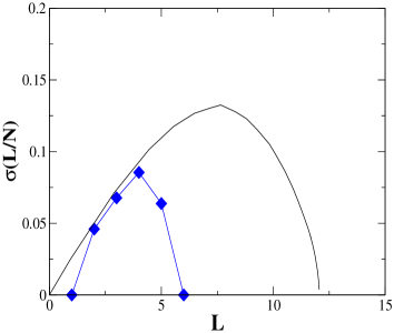
Figure 1: Entropy $\sigma(L/N)$ of the loops of length $L$ for the real Chesapeake food-web (solid line) and the entropy of the loops counted by exact enumeration (diamods).

5 Application of the algorithm to real directed networks

We applied the formulated algorithm to a large set of directed networks [17]. For some of these networks we calculated the number of loops ${\cal N}_{L}$ of lenght $L$ directly by exact enumeration [12]. We then compare the entropy of the loops $\sigma(\ell)$ find by the BP algorithm with the entropy of the loops $\sigma_{0}(\ell)$ find by directed enumeration of the number of loops

$$\sigma_{0}(\ell)=\frac{1}{N}\ln({\cal N}_{L=\ell N}^{\mbox{exact}})$$ (29)

We note that for the foodweb with small number of nodes the algorithm does not provide a good approximation for the number of loops present in the graph. A dramatic example is the Chesapeake foodweb. In this case we were able to count all the loops in the network exhaustively since the network contains very few loops. In this case the BP algorithm since the loops are few the BP algorithm highly overestimates the largest loop in the network (See Figure 1). In fact it predict a largest loop of lend $L_{max}=12$ where the largest loop is of length $L_{max}=7$. This effect is observed to be present also in the undirected BP algorithm [14].

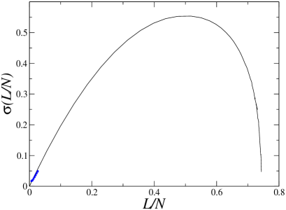
Figure 2: Entropy $\sigma(L/N)$ of the loops of length $L$ for the real C.elegans neural network (solid line) and the entropy of the loops counted by exact enumeration for small loops (small diamods).

The discrepancy is predicted to be strong only in cases where the size of the network is small and the number of loops in the network is small just as in the Chesapeake case. When the network has a larger number of loops and the entropy of the loops is larger, much better results are expected. In the case of the C. elegans neural network ($N=306$) the entropy for small number of loops is overlapping with the results of exact enumeration as it can clearly be seen in Figure 2. We further compare the results of the algorithm on a given network and on randomized network ensemble. A typical example is the metabolic network of E. coli [17] in which we could compare the entropy provided by the BP algorithm with the entropy of a series of $100$ random network with the same degree distribution.

6 Conclusions

In conclusion we provide a new algorithm for counting large loops in directed network. The algorithm is predicted to give good results only for large networks size $N$. In the paper we demonstrate cases in which it fails to predict the right entropy and loop structure due to the small size of the network. We propose to study the significance of loops structure in large networks by comparing the results of the algorithm on real networks and randomized networks when networks are large an the number of loops in the network are also large.

7 Acknowledgment

We acknowledge G. Semerjian and A. E. Motter for interesting discussions.

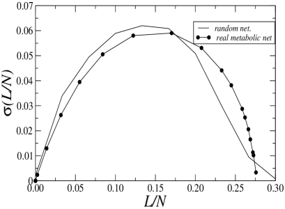
Figure 3: Entropy $\sigma(L/N)$ of the loops of length $L$ for the real metabolic network and average entropy of the loops in the randomized network ensemble with same degree sequence.

References

• [1] S. N. Dorogovtsev, A. V. Goltsev and J. F. F. Mendes, arXiv:0705.0010 (2007).
• [2] A. E. Motter, M. A. Matias, J. Kurths and E. Ott, Physica D 224,vii (2006).
• [3] Z. Toroczkai and K. E. Bassler, Nature (London) 428, 716 (2004).
• [4] T. Nishikawa and A. E. Motter, Physica D 224, 77 (2006).
• [5] T. Galla, J. Phys. A 39, 3853 (2006).
• [6] K. Klemm and S. Bornholdt, Proc. Natl Acad. Sci. U.S.A. 102, 18414 (2005)
• [7] G. Bianconi, N. Gulbahce and A. E. Motter, arXiv:0707.4084 (2007).
• [8] D. J. Watts and S. H. Strogatz, Nature (London) 393, 440 (1998).
• [9] G. Bianconi and A. Capocci, Phys. Rev. Lett. 90 , 078701 (2003).
• [10] G. Bianconi and M. Marsili, J. Stat. Mech. P06005 (2005).
• [11] D. B. Johnson, SIAM J. Comput. 4 77 (1975).
• [12] R. Tarjan, SIAM J. Compt. 2, 211 (1973).
• [13] H. D. Rozenfeld,J. E. Kirk, E. M. Bollt and D. ben-Avraham, J. Phys. A 38, 4589 (2005).
• [14] E. Marinari, R. Monasson and G. Semerjian, Europhys. Lett. 73,8 (2006).
• [15] E. Marinari and G. Semerjian, J. Stat. Mech. P06019 (2006).
• [16] Z. Burda and A. Krzywicki, Phys. Rev. E 67, 046118 (2003); M. Boguñá, R. Pastor-Satorras, and A. Vespignani, Eur. Phys. J. B 38, 205 (2004).
• [17] The network data are available at http://vlado.fmf.unilj.si/pub/networks/data/ (Chesapeake and Mondego foodwebs), www.cosinproject.org/ (Littlerock and Seagrass foodwebs), http://cdg.columbia.edu/cdg/ (C. elegans neural network), and www.weizmann.ac.il/mcb/UriAlon/ (S. cerevisiae transcription network). The Texas power-grid dataset was provided by Ken Werley (LANL), and the E. coli metabolic network was generated using flux balance analysis [18] on the reconstructed metabolic model iJE660 available at http://gcrg.ucsd.edu/organisms/. We consider the metabolic network without the metabolites $\rm CO_{2}$, $\rm NH_{3}$, $\rm PP_{i}$, $\rm P_{i}$, $\rm ATP$, $\rm ADP$, $\rm NAD$, $\rm NADP$, and $\rm NADH$, as in D. A. Fell and A. Wagner, Nat. Biotech. 18, 1121 (2000).
• [18] J. S. Edwards and B. O. Palsson, Proc. Natl Acad. Sci. U.S.A. 97, 5528 (2000).