Computing Knot Floer Homology in Cyclic Branched Covers

Abstract.

We use grid diagrams to give a combinatorial algorithm for computing the knot Floer homology of the pullback of a knot $K$ in its $m$-fold cyclic branched cover $\Sigma^{m}(K)$, and we give computations when $m=2$ for over fifty three-bridge knots with up to eleven crossings.

1. Introduction

Heegaard Floer knot homology, developed by Ozsváth and Szabó [14] and independently by Rasmussen [18], associates to a knot $K$ in a three-manifold $Y$ a bigraded group $\widehat{\operatorname{HFK}}(Y,K)$ that is an invariant of the knot type of $K$. If $K$ is a knot in $S^{3}$, then the inverse image of $K$ in $\Sigma^{m}(K)$, the $m$-fold cyclic branched cover of $S^{3}$ branched along $K$, is a nulhomologous knot $\tilde{K}$ whose knot type depends only on the knot type of $K$, so the group $\widehat{\operatorname{HFK}}(\Sigma^{m}(K),\tilde{K})$ is a knot invariant of $K$. In this paper, we describe an algorithm that can compute $\widehat{\operatorname{HFK}}(\Sigma^{m}(K),\tilde{K})$ (with coefficients in $\mathbb{Z}/2$) for any knot $K\subset S^{3}$, and we give computations for a large collection of knots with up to eleven crossings.

Any knot $K\subset S^{3}$ can be represented by means of a grid diagram, consisting of an $n\times n$ grid in which the centers of certain squares are marked $X$ or $O$, such that each row and each column contains exactly one $X$ and one $O$. To recover a knot projection, draw an arc from the $X$ and the $O$ in each column and from the $O$ to the $X$ in each row, making the vertical strand pass over the horizontal strand at each crossing. We may view the diagram as lying on a standardly embedded torus $T^{2}\subset S^{3}$ by making the standard edge identifications; the horizontal grid lines become $\alpha$ circles and the vertical ones $\beta$ circles. Manolescu, Ozsváth, and Sarkar [12] showed that such diagrams can be used to compute $\widehat{\operatorname{HFK}}(S^{3},K)$ combinatorially; we shall use them to compute $\widehat{\operatorname{HFK}}(\Sigma^{m}(K),\tilde{K})$ for any knot $K\subset S^{3}$. (See also [1, 13, 21].)

Let $\tilde{T}$ be the surface obtained by gluing together $m$ copies of $T$ (denoted $T_{0},\dots,T_{m-1}$) along branch cuts connecting the $X$ and the $O$ in each column. Specifically, in each column, if the $X$ is above the $O$, then glue the left side of the branch cut in $T_{k}$ to the right side of the same cut in $T_{k+1}$ (indices modulo $m$); if the $O$ is above the $X$, then glue the left side of the branch cut in $T_{k}$ to the right side of the same cut in $T_{k-1}$. The obvious projection $\pi:\tilde{T}\to T$ is an $m$-fold cyclic branched cover, branched around the marked points. Each $\alpha$ and $\beta$ circle in $T$ intersects the branch cuts a total of zero times algebraically and therefore has $m$ distinct lifts to $T$, and each lift of each $\alpha$ circle intersects exactly one lift of each $\beta$ circle. (We will describe these intersections more explicitly in Section 4.)

Denote by $\mathcal{R}$ the set of embedded rectangles in $T$ whose lower and upper edges are arcs of $\alpha$ circles, whose left and right edges are arcs of $\beta$ circles, and which do not contain any marked points in their interior. Each rectangle in $\mathcal{R}$ has $m$ distinct lifts to $\tilde{T}$ (possibly passing through the branch cuts as in Figure 1); denote the set of such lifts by $\tilde{\mathcal{R}}$.

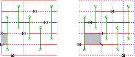
Figure 1. Heegaard diagram $\tilde{D}=(\tilde{T},\tilde{\bm{\alpha}},\tilde{\bm{\beta}},\tilde{\mathbf{w}},\tilde{\mathbf{z}})$ for $(\Sigma^{2}(K),\tilde{K})$, where $K$ is the right-handed trefoil. The solid and dashed lines represent different lifts of the $\alpha$ (horizontal/red) and $\beta$ (vertical/blue) circles. The black squares and crosses represent two generators of $\tilde{C}=\widehat{\operatorname{CFK}}(\tilde{\mathcal{D}})$, and the shaded region is a disk that contributes to the differential.

Let $\SS$ be the set of unordered $mn$-tuples $\mathbf{x}$ of intersection points between the lifts of $\alpha$ and $\beta$ circles such that each such lift contains exactly one point of $\mathbf{x}$. (We will give a more explicit characterization of the elements of $\SS$ later.) Let $C$ be the $\mathbb{Z}/2$-vector space generated by $\SS$. Define a differential $\partial$ on $C$ by making the coefficient of $\mathbf{y}$ in $\tilde{\partial}\mathbf{x}$ nonzero if and only if the following conditions hold:

• All but two of the points in $\mathbf{x}$ are also in $\mathbf{y}$.

• There is a rectangle $R\in\tilde{\mathcal{R}}$ whose lower-left and upper-right corners are in $\mathbf{x}$, whose upper-left and lower-right corners are in $\mathbf{y}$, and which does not contain any point of $\mathbf{x}$ in its interior.

In Section 4, we shall define two gradings (Alexander and Maslov) on $C$, as well as a decomposition of $C$ as a direct sum of complexes corresponding to spin^c structures on $\Sigma^{m}(K)$. We shall prove:

Theorem 1.

The homology of the complex $(C,\partial)$ is isomorphic as a bigraded group to $\widehat{\operatorname{HFK}}(\Sigma^{m}(K),\tilde{K};\mathbb{Z}/2)\otimes V^{\otimes n-1}$, where $V\cong\mathbb{Z}/2\oplus\mathbb{Z}/2$ with generators in bigradings $(0,0)$ and $(-1,-1)$.

In Section 2, we review the construction of Heegaard Floer homology for knots using multi-pointed Heegaard diagrams. In Section 3, we show how to obtain a Heegaard diagram for $(\Sigma^{m}(K),\tilde{K})$ given one for $(S^{3},K)$, and we use apply that discussion to grid diagrams in Section 4, proving Theorem 1. In Section 5, we give the values of $\widehat{\operatorname{HFK}}(\Sigma^{m}(K),\tilde{K})$ for over fifty knots with up to eleven crossings. (Grigsby [6] has shown how to compute these groups for two-bridge knots, so our tables only include knots that are not two-bridge.) Finally, we make some observations and conjectures about these results in Section 6.

Acknowledgments. I am grateful to Peter Ozsváth for suggesting this problem, providing lots of guidance, and reading a draft of this paper, and to John Baldwin, Tom Peters, Josh Greene, Matthew Hedden, and especially Eli Grigsby for many extremely helpful conversations.

2. Review of Heegaard Floer homology for knots

Let us briefly recall the basic construction of Heegaard Floer homology for knots [14]. For simplicity, we work with coefficients modulo 2. A multi-pointed Heegaard diagram $\mathcal{D}=(\Sigma,\bm{\alpha},\bm{\beta},\mathbf{w},\mathbf{z})$ consists of an oriented surface $\Sigma$; two sets of closed, embedded curves $\bm{\alpha}=\{\alpha_{1},\dots,\alpha_{g+n-1}\}$ and $\bm{\beta}=\{\beta_{1},\dots,\beta_{g+n-1}\}$ (where $g=g(\Sigma)$ and $n\geq 1$), each of which spans a $g$-dimensional subspace of $H_{1}(\Sigma;\mathbb{Z})$; and two sets of basepoints, $\mathbf{w}=\{w_{1},\dots,w_{n}\}$ and $\mathbf{z}=\{z_{1},\dots,z_{n}\}$, such that each component of $\Sigma-\bigcup\alpha_{i}$ and each component of $\Sigma-\bigcup\beta_{i}$ contains exactly one point of $\mathbf{w}$ and one point of $\mathbf{z}$. We obtain an oriented 3-manifold $Y$ and a handlebody decomposition $Y=H_{\alpha}\cup_{\Sigma}H_{\beta}$ by attaching 2-handles to $\Sigma\times I$ along the circles $\alpha_{i}\times\{0\}$ and $\beta_{i}\times\{1\}$ and then canonically filling in 3-balls. To obtain a knot or link $K$, we connect the $w$ (resp. $z$) basepoints to the $z$ (resp. $w$) basepoints with arcs in the complement of the $\alpha$ (resp. $\beta$) curves and push those arcs into $H_{\alpha}$ (resp. $H_{\beta}$). The orientations are such that $K$ intersects $\Sigma$ positively at the $z$ basepoints (where it is passing from $H_{\alpha}$ to $H_{\beta}$) and negatively at the $w$ basepoints (where it is passing from $H_{\beta}$ to $H_{\alpha}$).

In terms of Morse theory, we obtain a Heegaard diagram for a given pair $(Y,K)$ by taking a self-indexing Morse function $f$ on $Y$ and a Riemannian metric such that $K$ is a union of gradient flowlines connecting all the index-0 and index-3 basepoints. We then define $\Sigma$ as $f^{-1}(\frac{3}{2})$, the $\alpha$ (resp. $\beta$) circles as the intersections of $\Sigma$ with the ascending (resp. descending) manifolds of index-1 (resp. index-2) critical points of $f$, and the $w$ (resp. $z$) basepoints as the intersections of $\Sigma$ with the segments of $K$ that go from the index-3 (resp. index-0) critical points to the index-0 (resp. index-3) critical points. We then have $H_{\alpha}=f^{-1}([0,\frac{3}{2}])$ and $H_{\beta}=f^{-1}([\frac{3}{2},3])$.

The Heegaard Floer complex $\widehat{\operatorname{CFK}}(\mathcal{D})$ is defined as follows. Let $\mathbb{T}_{\alpha}$ and $\mathbb{T}_{\beta}$ be the images of $\alpha_{1}\times\dots\times\alpha_{g+n-1}$ and $\beta_{1}\times\dots\times\beta_{g+n-1}$ in the symmetric product $\operatorname{Sym}^{g+n-1}(\Sigma)$; these are both embedded copies of $T^{g+n-1}$. The group $\widehat{\operatorname{CFK}}(\mathcal{D})$ is the $\mathbb{Z}/2$-vector space generated by the (finitely many) intersection points in $\mathbb{T}_{\alpha}\cap\mathbb{T}_{\beta}$, and the differential $\partial$ is defined by taking counts of holomorphic disks connecting intersection points:

$$\partial\mathbf{x}=\sum_{\mathbf{y}\in\mathbb{T}_{\alpha}\cap\mathbb{T}_{\beta}}\sum_{\begin{subarray}{c}\phi\in\pi_{2}(\mathbf{x},\mathbf{y})\mid\\ \mu(\phi)=1\\ n_{w}(\phi)=n_{z}(\phi)=0\end{subarray}}\#\left(\frac{\mathcal{M}(\phi)}{\mathbb{R}}\right)\mathbf{y}.$$

Each homotopy class of Whitney disks $\phi\in\pi_{2}(\mathbf{x},\mathbf{y})$ has an associated domain in $\Sigma$: a 2-chain $D=\sum a_{i}D_{i}$, where the $D_{i}$ are components of $\Sigma-\bigcup\alpha_{i}-\bigcup\beta_{i}$ (elementary domains), such that $\partial D$ is made of arcs of $\alpha$ curves that connect each point of $\mathbf{x}$ to a point of $\mathbf{y}$ and arcs of $\beta$ curves that connect each point of $\mathbf{y}$ to a point of $\mathbf{x}$. Then $n_{\mathbf{w}}(\phi)$ and $n_{\mathbf{z}}(\phi)$ are the multiplicities of the elementary domains containing points of $\mathbf{w}$ and $\mathbf{z}$, respectively. The Maslov index $\mu(\phi)$ can be computed using a formula due to Lipshitz [10]:

$$\mu(\phi)=\sum_{i}a_{i}e(D_{i})+p_{\mathbf{x}}(D)+p_{\mathbf{y}}(D),$$

where $p_{\mathbf{x}}(D)$ (resp. $p_{\mathbf{y}}(D)$) equals the sum of the average of the multiplicities of the domains at the four corners of each point of $\mathbf{x}$ (resp. $\mathbf{y}$), and $e(D_{i})$, the Euler measure, equals $1-\frac{k}{2}$ when $D_{i}$ is a convex $2k$-gon. The coefficient of $\mathbf{y}$ represents the number of holomorphic representatives of $\phi$ and generally depends on the choice of almost complex structure on $\Sigma$. For suitable choices, the homology of the complex is then isomorphic to $\widehat{\operatorname{HFK}}(Y,K)\otimes V^{\otimes n-1}$, where $V\cong\mathbb{Z}/2\oplus\mathbb{Z}/2$ with generators in bigradings $(-1,-1)$ and $(0,0)$, and $\widehat{\operatorname{HFK}}(Y,K)$ is an invariant of the knot type of $K\subset Y$.

To define the spin^c structure $\mathfrak{s}_{\mathbf{w}}(\mathbf{x})$ associated to a generator $\mathbf{x}$, let $N_{\mathbf{x}}$ be the union of regular neighborhoods of the closures of the gradient flowlines through the points of $\mathbf{x}$ and $\mathbf{w}$. (Flowlines through the former connect index-1 and index-2 critical points of $f$; those through the latter connect index-0 and index-3 critical points.) The gradient vector field $\vec{\nabla}f$ is non-vanishing on $Y-N_{\mathbf{x}}$ and hence defines a spin^c structure (using Turaev’s formulation of spin^c structures as homology classes of non-vanishing vector fields [22]). Let $\widehat{\operatorname{CFK}}(\mathcal{D},\mathfrak{s})\subset\widehat{\operatorname{CFK}}(\mathcal{D})$ be the subspace generated by the generators $\mathbf{x}$ with $\mathfrak{s}_{\mathbf{w}}(\mathbf{x})=\mathfrak{s}$. To test whether two generators $\mathbf{x}$ and $\mathbf{y}$ are in the same spin^c structure, let $\gamma_{\mathbf{x},\mathbf{y}}$ be a 1-cycle obtained by connecting $\mathbf{x}$ to $\mathbf{y}$ along the $\alpha$ circles and $\mathbf{y}$ to $\mathbf{x}$ along the $\beta$ circles, and let $\epsilon(\mathbf{x},\mathbf{y})$ be its image in

$$H_{1}(Y)\cong H_{1}(\Sigma)/\operatorname{Span}([\alpha_{i}],[\beta_{i}]\mid i=1,\dots,g+n-1).$$

Then $\mathbf{x}$ and $\mathbf{y}$ are in the same spin^c structure if and only if $\epsilon(\mathbf{x},\mathbf{y})=0$. In particular, if $\mathbf{y}$ appears in the boundary of $\mathbf{x}$, then $\epsilon(\mathbf{x},\mathbf{y})=0$, so $\widehat{\operatorname{CFK}}(\mathcal{D},\mathfrak{s})$ is a subcomplex. The homology of each of these summands does not depend on the choice of complex, so there is a natural splitting

$$\widehat{\operatorname{HFK}}(Y,K)=\bigoplus_{\mathfrak{s}\in\operatorname{Spin}^{c}(Y)}\widehat{\operatorname{HFK}}(Y,K,\mathfrak{s}).$$

If $K$ is nulhomologous, the Alexander grading on $\widehat{\operatorname{CFK}}(Y,K)$ is defined as follows. For each generator $\mathbf{x}$, let $\underline{\mathfrak{s}}_{\mathbf{w},\mathbf{z}}(\mathbf{x})\in\underline{\operatorname{Spin}^{c}}(Y,K)=\operatorname{Spin}^{c}(Y_{0}(K))$ be the spin^c structure on the zero-surgery $Y_{0}(K)$ obtained by extending $\mathfrak{s}_{\mathbf{w}}(\mathbf{x})|_{Y-N(K)}$ over $Y_{0}(K)$. Given a Seifert surface $F$ for $K$, the Alexander grading of $\mathbf{x}$ is $A_{F}(\mathbf{x})=\frac{1}{2}\left\langle c_{1}(\underline{\mathfrak{s}}_{\mathbf{w},\mathbf{z}}(\mathbf{x})),[\hat{F}]\right\rangle$, where $\hat{F}$ is the capped-off Seifert surface in $Y_{0}(K)$. The Alexander grading is always independent of the choice of $F$ up to an additive constant and completely independent when $Y$ is a rational homology sphere. The relative Alexander grading between two generators $\mathbf{x}$ and $\mathbf{y}$, $A(\mathbf{x},\mathbf{y})=A(\mathbf{x})-A(\mathbf{y})$, can also be given as the linking number of $\gamma_{\mathbf{x},\mathbf{y}}$ and $K$ (i.e., the intersection number of $\gamma_{\mathbf{x},\mathbf{y}}$ with $F$), or by the formula $A(\mathbf{x},\mathbf{y})=n_{\mathbf{z}}(D)-n_{\mathbf{w}}(D)$ when $\mathbf{x}$ and $\mathbf{y}$ are in the same spin^c structure and $\mathcal{D}$ is any domain connecting $\mathbf{x}$ to $\mathbf{y}$. The latter formula shows that the complex $\widehat{\operatorname{CFK}}(\mathcal{D},\mathfrak{s})$ splits according to Alexander gradings, and hence

$$\widehat{\operatorname{HFK}}(Y,K,\mathfrak{s})=\bigoplus_{i\in\mathbb{Z}}\widehat{\operatorname{HFK}}(Y,K,\mathfrak{s},i).$$

If $\mathfrak{s}\in\operatorname{Spin}^{c}(Y)$ is a torsion spin^c structure, the relative Maslov grading between two generators $\mathbf{x}$ and $\mathbf{y}$ with $\mathfrak{s}_{\mathbf{w}}(\mathbf{x})=\mathfrak{s}_{\mathbf{w}}(\mathbf{y})=\mathfrak{s}$ is given by $M(\mathbf{x},\mathbf{y})=\mu(D)-2n_{\mathbf{w}}(D)$, where $D$ is any domain connecting $\mathbf{x}$ to $\mathbf{y}$. An easy way to compute the relative Maslov grading between two generators in the same spin^c structure is to find a linear combination of $\alpha$ and $\beta$ circles that is homologous to $\gamma_{\mathbf{x},\mathbf{y}}$ (which is possible since $\gamma_{\mathbf{x},\mathbf{y}}\equiv 0$ in $H_{1}(Y)$). Then $\gamma_{\mathbf{x},\mathbf{y}}$ minus this linear combination bounds a domain $D$ in $\Sigma$ connecting $\mathbf{x}$ to $\mathbf{y}$, and we then apply Lipshitz’s formula to compute $\mu(D)$.

Moreover, if $Y$ is a rational homology sphere, the relative $\mathbb{Z}$-gradings on the $\widehat{\operatorname{CFK}}(Y,K,\mathfrak{s})$ lift to an absolute $\mathbb{Q}$-grading on all of $\widehat{\operatorname{CFK}}(Y,K)$. Lipshitz and Lee [9] show that it is easy to compute the relative $\mathbb{Q}$-grading between two generators that are not necessarily in the same spin^c structure. Since $H_{1}(Y)$ is finite, there exists $m\geq 1$ such that $m\gamma_{\mathbf{x},\mathbf{y}}$ is homologous to a linear combination of $\alpha$ and $\beta$ circles, so $m\gamma_{\mathbf{x},\mathbf{y}}$ minus this combination bounds a domain $D$. The relative Maslov $\mathbb{Q}$-grading between $\mathbf{x}$ and $\mathbf{y}$ is then $M(\mathbf{x},\mathbf{y})=\frac{1}{m}(\mu(D)-2n_{\mathbf{w}}(D))$. The absolute $\mathbb{Q}$-grading is more complicated, and we shall not discuss it in this paper.

Call a diagram $\mathcal{D}$ good if every elementary domain that does not contain a basepoint is either a bigon or a square. Manolescu, Ozsváth, and Sarkar showed that in any good diagram, the coefficient of $\mathbf{y}$ in $\partial\mathbf{x}$ is nonzero in two cases:

• All but one of the points of $\mathbf{y}$ are also in $\mathbf{x}$, and the remaining two points are the vertices of a bigon without a basepoint or a point of $\mathbf{x}$ in its interior.

• All but two of the points of $\mathbf{y}$ are also in $\mathbf{x}$, and the remaining four points are the vertices of a rectangle without a basepoint or a point of $\mathbf{x}$ in its interior.

It follows that when $\mathcal{D}$ is a good diagram, the boundary map can be determined simply from the combinatorics of the diagram, without reference to the choice of complex structure on $\Sigma$, so $\widehat{\operatorname{HFK}}(Y,K)$ can be computed algorithmically.

If $K$ is a knot in $S^{3}$, then a grid diagram for $K$, drawn on a torus as in Section 1, yields a Heegaard diagram $\mathcal{D}=(T^{2},\bm{\alpha},\bm{\beta},\mathbf{w},\mathbf{z})$ for the pair $(S^{3},K)$, where the $\alpha$ circles are the horizontal lines of the grid, the $\beta$ circles are the vertical lines, and the $w$ and $z$ basepoints are the points marked $O$ and $X$, respectively. Every region of this diagram is a square, so $\widehat{\operatorname{HFK}}(S^{3},K)$ can be computed combinatorially as above. Specifically, the generators correspond to permutations of the set $\{1,\dots,n\}$, and the Alexander and Maslov gradings of each generator can be given by simple formulae (discussed later). Using this diagram, Baldwin and Gillam [1] have computed $\widehat{\operatorname{HFK}}(S^{3},K)$ for all knots with up to 12 crossings. Additionally, Manolescu, Ozsváth, Szabó, and Thurston [13] give a self-contained proof that this construction yields a knot invariant. (See also Sarkar and Wang [21], who show how to obtain good diagrams for knots in arbitrary 3-manifolds.)

3. Heegaard diagrams for cyclic branched covers of knots

Given a knot $K\subset S^{3}$ and an integer $m\geq 2$, there is a well-known construction of a 3-manifold $\Sigma^{m}(K)$ and an $m$-fold branched covering map $\pi:\Sigma^{m}(K)\to S^{3}$ whose downstairs branch locus is $K$ and whose upstairs branch locus is a knot $\tilde{K}\subset\Sigma^{m}(K)$. The manifold $\Sigma^{m}(K)$ can be constructed from $m$ copies of $S^{3}-\operatorname{int}F$, where $F$ is a Seifert surface for $K$, by connecting the negative side of a bicollar of $F$ in the $k^{\text{th}}$ copy to the positive side in the $(k+1)^{\text{th}}$ (indices modulo $m$). The inverse image of $K$ in $\Sigma^{m}(K)$ is a knot $\tilde{K}$, which is nulhomologous because it bounds a Seifert surface (any of the lifts of the original Seifert surface $F$). For the details of this construction, see Rolfsen [20].

The group of covering transformations of $\Sigma^{m}(K)\to S^{3}$ is cyclic of order $m$, generated by a map $\tau_{m}:\Sigma^{m}(K)\to\Sigma^{m}(K)$ that takes the $k^{\text{th}}$ copy of $S^{3}\smallsetminus\operatorname{int}F$ to the $(k+1)^{\text{th}}$ (indices modulo $m$). If $\gamma$ is a $1$-cycle in $S^{3}$, then by using transfer homomorphisms, we see that for any lift $\tilde{\gamma}$, the equation

(1) $$\sum_{k=0}^{m-1}\tau_{m*}^{k}(\tilde{\gamma})=0$$

holds in $H_{1}(\Sigma^{m}(K);\mathbb{Z})$. In particular, when $m=2$, we have $\tau_{2*}(\tilde{\gamma})=-\tilde{\gamma}$.

When $m$ is a power of a prime $p$, the group $H_{1}(\Sigma^{m}(K);\mathbb{Z})$ is then finite and contains no $p^{r}$-torsion for any $r$ [4, p. 16]. The order of $H_{1}(\Sigma^{m}(K))$ is equal to $\prod_{j=0}^{m-1}\Delta_{K}(\omega^{j})$, where $\Delta_{K}$ is the Alexander polynomial of $K$, and $\omega$ is a primitive $m^{\text{th}}$ root of unity [2, p. 149]. In particular, note that the action of the deck transformation group on $H_{1}(\Sigma^{m}(K);\mathbb{Z})$ has no nonzero fixed points: if $\tau_{m*}(\alpha)=\alpha$, then

$$0=\alpha+\tau_{m*}(\alpha)+\dots+\tau_{m*}^{m-1}(\alpha)=m\alpha,$$

by Equation 1, so $\alpha=0$.

Let $\mathcal{D}=(S,\bm{\alpha},\bm{\beta},\mathbf{w},\mathbf{z})$ be a multi-pointed Heegaard diagram for $K\subset S^{3}$ with genus $g$ and $n$ basepoint pairs. If $f:S^{3}\to\mathbb{R}$ is a self-indexing Morse function compatible with $\mathcal{D}$, then $\tilde{f}=f\circ\pi:\Sigma^{m}(K)\to\mathbb{R}$ is a self-indexing Morse function for the pair $(\Sigma^{m}(K),\tilde{K})$ whose critical points are simply the inverse images of the critical points of $f$. This function induces a Heegaard splitting $\Sigma^{m}(K)=\tilde{H}_{\alpha}\cup_{\tilde{S}}\tilde{H}_{\beta}$ that projects onto the Heegaard splitting of $S^{3}$. A simple Euler characteristic argument shows that the genus of the new Heegaard surface $\tilde{S}=\pi^{-1}(S)$ is $h=mg+(m-1)(n-1)$. Each $\alpha$ and $\beta$ circle in $S$ bounds a disk in $S^{3}\smallsetminus K$ and hence has $m$ distinct preimages in $\Sigma^{m}(K)$. Thus, we obtain a Heegaard diagram $\tilde{\mathcal{D}}=(\tilde{S},\tilde{\bm{\alpha}},\tilde{\bm{\beta}},\tilde{\mathbf{w}},\tilde{\mathbf{z}})$, where $\tilde{S}$ is a surface of genus $h$ and $\tilde{\bm{\alpha}},\tilde{\bm{\beta}},\tilde{\mathbf{w}},\tilde{\mathbf{z}}$ are the inverse images of the corresponding objects under the covering map.

We may arrange that the Heegaard surface $F$ intersects $S$ in $n$ arcs, each connecting a $z$ basepoint to a $w$ basepoint. Note that each $\alpha$ or $\beta$ circle intersects $F$ algebraically zero times, since, e.g., $\alpha_{i}\cdot F=\operatorname{lk}(\alpha_{i},K)=K\cdot D_{\alpha_{i}}=0$, where $D_{\alpha_{i}}$ is a spanning disk for $\alpha_{i}$. To obtain the diagram $\tilde{\mathcal{D}}$ directly, we may connect $m$ copies of $\mathcal{D}$ by using the arcs of $F\cap S$ as branch cuts. A complex structure on $S$ naturally yields a complex structure on $\tilde{S}$ that makes the projection $\pi:\tilde{S}\to S$ and the covering transformation $\tau_{m}:\tilde{S}\to\tilde{S}$ holomorphic.

The generators of the complex $\widehat{\operatorname{CFK}}(\tilde{\mathcal{D}})$ may be described as follows:

Lemma 3.1.

Any generator $\mathbf{x}$ of $\widehat{\operatorname{CFK}}(\tilde{\mathcal{D}})$ can be decomposed (non-uniquely) as $\mathbf{x}=\tilde{\mathbf{x}}_{1}\cup\dots\cup\tilde{\mathbf{x}}_{m}$, where $\mathbf{x}_{1},\dots,\mathbf{x}_{m}$ are generators of $\widehat{\operatorname{CFK}}(\mathcal{D})$, and $\tilde{\mathbf{x}}_{i}$ is a lift of $\mathbf{x}_{i}$ to $\tilde{\mathcal{D}}$.

Proof.

Given a generator $\mathbf{x}$ of $\widehat{\operatorname{CFK}}(\tilde{\mathcal{D}})$, let $\bar{\mathbf{x}}$ be its image under the natural map $\operatorname{Sym}^{mn}(\tilde{S})\to\operatorname{Sym}^{mn}(S)$, consisting of $mn$ points of $\Sigma$ (possibly repeated) such that each $\alpha$ circle and each $\beta$ circle contains exactly $m$ points. It is then easy to partition $\bar{\mathbf{x}}$ into $m$ subsets $\mathbf{x}_{1},\dots,\mathbf{x}_{m}$, each of which is a generator of $\widehat{\operatorname{CFK}}(\mathcal{D})$ as required. Note that this choice of partition is not unique. ∎

Given a generator $\mathbf{x}_{0}$ of $\widehat{\operatorname{CFK}}(\mathcal{D})$, let $L(\mathbf{x}_{0})$ denote the generator of $\widehat{\operatorname{CFK}}(\tilde{\mathcal{D}})$ consisting of all $m$ lifts of each point of $\mathbf{x}_{0}$. Using the action of the deck transformation $\tau_{m}$ on $\mathcal{D}$, we may write $L(\mathbf{x}_{0})=\tilde{\mathbf{x}}_{0}\cup\tau_{m}(\tilde{\mathbf{x}}_{0})\cup\dots\cup\tau_{m}^{m-1}(\tilde{\mathbf{x}})$, where $\tilde{\mathbf{x}}_{0}$ is any lift of $\mathbf{x}_{0}$ to $\tilde{D}$.

Lemma 3.2.

All generators of $\widehat{\operatorname{CFK}}(\tilde{\mathcal{D}})$ of the form $\mathbf{x}=L(\mathbf{x}_{0})$ are in the same spin^c structure, denoted $\mathfrak{s}_{0}$ and called the canonical spin^c structure on $\Sigma^{m}(K)$.

Proof.

(Adapted from Grigsby [5].) Let $\mathbf{x}_{0}$ and $\mathbf{y}_{0}$ be generators of $\widehat{\operatorname{CFK}}(\mathcal{D})$; we shall show that $L(\mathbf{x}_{0})$ and $L(\mathbf{y}_{0})$ are in the same spin^c structure. Let $\gamma_{\mathbf{x}_{0},\mathbf{y}_{0}}$ be a 1-cycle joining $\mathbf{x}_{0}$ and $\mathbf{y}_{0}$ as above, and let $\tilde{\gamma}_{\mathbf{x}_{0},\mathbf{y}_{0}}$ be a lift of $\gamma_{\mathbf{x}_{0},\mathbf{y}_{0}}$ to $\tilde{S}$. Then the 1-cycle

$$\tilde{\gamma}_{\mathbf{x}_{0},\mathbf{y}_{0}}+\tau_{m*}(\tilde{\gamma}_{\mathbf{x}_{0},\mathbf{y}_{0}})+\dots+\tau_{m*}^{m-1}(\tilde{\gamma}_{\mathbf{x}_{0},\mathbf{y}_{0}})$$

connects $L(\mathbf{x}_{0})$ and $L(\mathbf{y}_{0})$. Then $\epsilon(L(\mathbf{x}_{0}),L(\mathbf{y}_{0}))=0$ by Equation 1, so $L(\mathbf{x}_{0})$ and $L(\mathbf{y}_{0})$ are in the same spin^c structure. ∎

Remark 3.3.

When $K$ is a two-bridge knot and $m=2$, Grigsby shows that for a specific diagram $\mathcal{D}$, the map $L$ extends to an isomorphism of bigraded chain complexes $\widehat{\operatorname{CFK}}(\mathcal{D})\to\widehat{\operatorname{CFK}}(\tilde{D},\mathfrak{s}_{0})$. Therefore, for any two-bridge knot $K$, $\widehat{\operatorname{HFK}}(\Sigma^{2}(K),\tilde{K},\mathfrak{s}_{0})\cong\widehat{\operatorname{HFK}}(S^{3},K)$. In general, though, $L$ is not even a chain map.

The spin^c structure $\mathfrak{s}_{0}$ often also admits a more intrinsic characterization. Assume $m$ is a prime power. If $f:S^{3}\to\mathbb{R}$ is a self-indexing Morse function for $(S^{3},K)$ as above, then its pullback $\tilde{f}:\Sigma^{m}(K)\to\mathbb{R}$ is $\tau_{m}$-invariant. Using a Riemannian metric on $\Sigma^{m}(K)$ that is the pullback of a metric on $S^{3}$, the gradient $\vec{\nabla}\tilde{f}$ is $\tau_{m}$-invariant and projects onto $\vec{\nabla}f$, and the flowlines for $\tilde{f}$ are precisely the lifts of flowlines for $f$. If $N_{\mathbf{x}_{0}}$ is the union of neighborhoods of flowlines through the points of $\mathbf{x}_{0}$ and $\mathbf{w}$, where $\mathbf{x}_{0}$ is a generator of $\widehat{\operatorname{CFK}}(\mathcal{D})$, then $\pi^{-1}(N_{\mathbf{x}_{0}})$ is the union of neighborhoods of flowlines through the points of $L(\mathbf{x}_{0})$ and can be denoted $N_{L(\mathbf{x}_{0})}$ as in Section 2. By suitably modifying $\vec{\nabla}\tilde{f}$ on $N_{L(\mathbf{x}_{0})}$, we may obtain a $\tau_{m}$-invariant vector field that determines $\mathfrak{s}_{\tilde{\mathbf{w}}}(L(\mathbf{x}_{0}))=\mathfrak{s}_{0}$. It follows that $\mathfrak{s}_{0}$ is fixed under the action of $\tau_{m}$ on $\operatorname{Spin}^{c}(\Sigma^{m}(K))$. Now, if $\mathfrak{s}_{0}^{\prime}$ is another spin^c structure fixed under the action of $\tau_{m}$, then the difference between $\mathfrak{s}_{0}$ and $\mathfrak{s}_{0}^{\prime}$ is a class in $H_{1}(\Sigma^{m}(K);\mathbb{Z})$ that is fixed by $\tau_{m}$, hence equals zero. Thus, $\mathfrak{s}_{0}$ is uniquely characterized by the property that $\tau_{m}^{*}(\mathfrak{s}_{0})=\mathfrak{s}_{0}$. For more about the significance of $\mathfrak{s}_{0}$, see [7].

We now consider the Alexander gradings in $\widehat{\operatorname{CFK}}(\tilde{\mathcal{D}})$.

Proposition 3.4.

If $\mathbf{x}=\tilde{\mathbf{x}}_{1}\cup\dots\cup\tilde{\mathbf{x}}_{m}$ as in Lemma 3.1, then the Alexander grading of $\mathbf{x}$ (computed with respect to a Seifert surface for $\tilde{K}$ that is a lift of a Seifert surface for $K$) is equal to the average of the Alexander gradings of $\mathbf{x}_{1},\dots,\mathbf{x}_{m}$.

Proof.

We first consider the relative Alexander gradings. Let $F\subset S^{3}$ be a Seifert surface for $K$, and let $\tilde{F}$ be a lift of $F$ to $\Sigma^{m}(K)$. The translates $\tilde{F},\tau_{m}(\tilde{F}),\dots,\tau_{m}^{m-1}(\tilde{F})$ are all Seifert surfaces for $\tilde{K}$. The relative Alexander grading between two generators does not depend on the choice of Seifert surface, so for generators $\mathbf{x},\mathbf{y}$ of $\widehat{\operatorname{CFK}}(\tilde{D})$, we have

$$mA(\mathbf{x},\mathbf{y})=\gamma_{\mathbf{x},\mathbf{y}}\cdot\tilde{F}+\gamma_{\mathbf{x},\mathbf{y}}\cdot\tau_{m}(\tilde{F})+\dots+\gamma_{\mathbf{x},\mathbf{y}}\cdot\tau_{m}^{m-1}(\tilde{F}),$$

where $\gamma_{\mathbf{x},\mathbf{y}}$ is a 1-cycle connecting $\mathbf{x}$ and $\mathbf{y}$ as above. The projection $\pi_{*}(\gamma_{\mathbf{x},\mathbf{y}})$ is a 1-cycle in $S$ that goes from $\bar{\mathbf{x}}$ to $\bar{\mathbf{y}}$ along $\alpha$ circles and from $\bar{\mathbf{y}}$ to $\bar{\mathbf{x}}$ along $\beta$ circles. Every intersection point of $\gamma_{\mathbf{x},\mathbf{y}}$ with one of the lifts of $F$ corresponds to an intersection point of $\pi_{*}(\gamma_{\mathbf{x},\mathbf{y}})$ with $F$, so

$$\gamma_{\mathbf{x},\mathbf{y}}\cdot\tilde{F}+\gamma_{\mathbf{x},\mathbf{y}}\cdot\tau_{m}(\tilde{F})+\dots+\gamma_{\mathbf{x},\mathbf{y}}\cdot\tau_{m}^{m-1}(\tilde{F})=\pi_{*}(\gamma_{\mathbf{x},\mathbf{y}})\cdot F.$$

The restriction of $\pi_{*}(\gamma_{\mathbf{x},\mathbf{y}})$ to any $\alpha$ or $\beta$ circle consists of $m$ (possibly constant or overlapping) arcs. By perhaps adding copies of the $\alpha$ or $\beta$ circle, we can arrange that these arcs connect a point of $\mathbf{x}_{1}$ with a point of $\mathbf{y}_{1}$, a point of $\mathbf{x}_{2}$ with a point of $\mathbf{y}_{2}$, and so on. In other words,

$$\pi_{*}(\gamma_{\mathbf{x},\mathbf{y}})\equiv\gamma_{\mathbf{x}_{1},\mathbf{y}_{1}}+\dots+\gamma_{\mathbf{x}_{m},\mathbf{y}_{m}}$$

modulo the $\alpha$ and $\beta$ circles in $\mathcal{D}$, whose intersection numbers with $F$ are zero. Therefore,

$$\begin{split}A(\mathbf{x},\mathbf{y})&=\frac{1}{m}(\gamma_{\mathbf{x}_{1},\mathbf{y}_{1}}+\dots,+\gamma_{\mathbf{x}_{m},\mathbf{y}_{m}})\cdot F\\ &=\frac{1}{m}(A(\mathbf{x}_{1},\mathbf{y}_{1})+\dots+A(\mathbf{x}_{m},\mathbf{y}_{m})).\end{split}$$

Thus, the Alexander grading of a generator of $\widehat{\operatorname{CFK}}(\tilde{\mathcal{D}})$ is given up to an additive constant by the average Alexander grading of its parts.

To pin down the additive constant, first note that the branched covering map $\pi:\Sigma^{m}(K)\to S^{3}$ extends to an unbranched covering map from the zero-surgery on $\tilde{K}$ to the zero-surgery on $K$, $\pi_{0}:\Sigma^{m}(K)_{0}\to S^{3}_{0}$. Since this is a local diffeomorphism, it is possible to pull back spin^c structures. Let $\mathbf{x}_{0}$ be a generator $\widehat{\operatorname{CFK}}(\mathcal{D})$ in Alexander grading 0, and let $\mathbf{x}=L(\mathbf{x}_{0})$. As in the discussion following Lemma 3.2, we may find a nonvanishing vector field that determines $\mathfrak{s}_{\tilde{\mathbf{w}}}(\mathbf{x})=\mathfrak{s}_{0}$ and is $\tau_{m}$-equivariant. The unique extension (up to isotopy) of this vector field to $\Sigma^{m}(K)_{0}$ can also be made $\tau_{m}$-invariant, so it is the pullback of an extension to $S^{3}_{0}$ of a vector field determining $\mathfrak{s}_{\mathbf{w}}(\mathbf{x}_{0})$. It follows that $\underline{\mathfrak{s}}_{\tilde{\mathbf{w}},\tilde{\mathbf{z}}}(\mathbf{x})=\pi_{0}^{*}(\underline{\mathfrak{s}}_{\mathbf{w},\mathbf{z}}(\mathbf{x}_{0}))$. Now, if $\hat{\tilde{F}}\subset Y_{0}(\tilde{K})$ is obtained by capping off $\tilde{F}$ in the zero-surgery, then $\pi_{0*}[\hat{\tilde{F}}]=[\hat{F}]$ in $H_{2}(S_{3}^{0};\mathbb{Z})$. Therefore,

$$\begin{split}A_{\tilde{F}}(\mathbf{x})&=\frac{1}{2}\left\langle c_{1}(\underline{\mathfrak{s}}_{\tilde{\mathbf{w}},\tilde{\mathbf{z}}}(\mathbf{x})),[\hat{\tilde{F}}]\right\rangle\\ &=\frac{1}{2}\left\langle c_{1}(\pi_{0}^{*}(\underline{\mathfrak{s}}_{\mathbf{w},\mathbf{z}}(\mathbf{x}_{0}))),[\hat{\tilde{F}}]\right\rangle\\ &=\frac{1}{2}\left\langle c_{1}(\underline{\mathfrak{s}}_{\mathbf{w},\mathbf{z}}(\mathbf{x}_{0})),\pi_{0*}[\hat{\tilde{F}}]\right\rangle\\ &=\frac{1}{2}\left\langle c_{1}(\underline{\mathfrak{s}}_{\mathbf{w},\mathbf{z}}(\mathbf{x}_{0})),[\hat{F}]\right\rangle\\ &=0=A_{F}(\mathbf{x}_{0}).\end{split}$$

Thus, the additive constant $C$ must equal 0. ∎

Next, we consider the domains in $\tilde{D}$. Any simply-connected elementary domain $D$ of $\mathcal{D}$ that does not contain a basepoint is evenly covered, so its preimage in $\tilde{\mathcal{D}}$ consists of $m$ disjoint domains each diffeomorphic to $D$. On the other hand, a domain containing exactly one basepoint is covered by a single connected domain with $m$ times as many sides as the original one. In particular, if $\mathcal{D}$ is a good diagram, then $\tilde{\mathcal{D}}$ is also good. It follows that the domains that count for the boundary in $\widehat{\operatorname{CFK}}(\tilde{\mathcal{D}})$ are precisely the lifts of the domains that count for the boundary of $\mathcal{D}$.

We conclude with a few comments about the symmetries in the case where $m=2$. The order of $H_{1}(\Sigma^{2}(K);\mathbb{Z})$ is equal to the determinant of $K$, $\det K=\Delta_{K}(-1)$, which is always odd. As mentioned above, the non-trivial deck transformation $\tau_{2}$ acts on $H_{1}(\Sigma^{2}(K);\mathbb{Z})$ by multiplication by $-1$. The set $\operatorname{Spin}^{c}(\Sigma^{2}(K))$ of spin^c structures on $\Sigma^{2}(K)$ is an affine set for $H_{1}(\Sigma^{2}(K);\mathbb{Z})$ and can be identified with the latter by sending the canonical spin^c structure $\mathfrak{s}_{0}$ to zero. Under this identification, both conjugation ($\mathfrak{s}\mapsto\bar{\mathfrak{s}}$) and pullback under $\tau_{2}$ ($\mathfrak{s}\mapsto\tau_{2}^{*}(\mathfrak{s})$) are given by with multiplication by $-1$, so $\tau_{2}^{*}(\mathfrak{s})=\bar{\mathfrak{s}}$. Since the diagram $\tilde{\mathcal{D}}$ is $\tau_{2}$-equivariant, $\tau_{2}$ induces an isomorphism of bigraded groups

$$\widehat{\operatorname{HFK}}(\Sigma^{2}(K),\tilde{K},\mathfrak{s})\to\widehat{\operatorname{HFK}}(\Sigma^{2}(K),\tilde{K},\bar{\mathfrak{s}}).$$

On the other hand, it is a standard fact [14, Prop. 3.10] that

$$\widehat{\operatorname{HFK}}_{j}(Y,K,\mathfrak{s},i)\cong\widehat{\operatorname{HFK}}_{j-2i}(Y,K,\bar{\mathfrak{s}},-i).$$

Therefore, to compute $\widehat{\operatorname{HFK}}(\Sigma^{2}(K),\tilde{K})$, it suffices to consider only one out of every pair of conjugate, non-canonical spin^c structures, and to consider only the generators that lie in non-negative Alexander grading. Additionally, note that since $\Sigma^{2}(K)$ is a rational homology sphere, the Maslov $\mathbb{Z}$-grading lifts to a $\mathbb{Q}$-grading that extends across all spin^c structures.

4. Grid diagrams and cyclic branched covers

As described in Section 1, any oriented knot $K\subset S^{3}$ can be represented by means of a grid diagram. By drawing the grid diagram on a standardly embedded torus in $S^{3}$, we may think of the grid diagram as a genus 1, multi-pointed Heegaard diagram $\mathcal{D}=(T^{2},\bm{\alpha},\bm{\beta},\mathbf{w},\mathbf{z})$ for the pair $(S^{3},K)$, where the $\alpha$ circles are the horizontal lines of the grid, the $\beta$ circles are the vertical lines, the $w$ basepoints are in the regions marked $O$, and the $z$ basepoints are in the regions marked $X$.

We label the $\alpha$ circles $\alpha_{0},\dots,\alpha_{n-1}$ from bottom to top and the $\beta$ circles $\beta_{0},\dots,\beta_{n-1}$ from left to right. Each $\alpha$ circle intersects each $\beta$ circle exactly once: $\beta_{i}\cap\alpha_{j}=\{x_{ij}\}$. Generators of the Heegaard Floer chain complex $\widehat{\operatorname{CFK}}(\mathcal{D})$ then correspond to permutations of the index set $\{0,\dots,n-1\}$ via the correspondence $\sigma\mapsto(x_{0,\sigma(0)},\dots,x_{n-1,\sigma(n-1)})$. The diagram is good, so the differential can be computed combinatorially as described in Section 2. Specifically, the coefficient of $\mathbf{y}$ in $\partial\mathbf{x}$ is 1 if all but two of the points of $\mathbf{x}$ and $\mathbf{y}$ agree and there is a rectangle embedded in the torus with points of $\mathbf{x}$ as its lower-left and upper-right corners, points of $\mathbf{y}$ as its lower-right and upper-left corners, and no basepoints or points of $\mathbf{x}$ in its interior, and 0 otherwise.

For each grid point $x$, let $w(x)$ denote the winding number of the knot projection around $x$. Let $p_{1},\dots,p_{8n}$ (repetitions allowed) denote the vertices of the $2n$ squares containing basepoints, and set

$$a=\frac{1-n}{2}+\frac{1}{8}\sum_{i=1}^{8n}w(p_{i}).$$

According to Manolescu, Ozsváth, and Sarkar [12], the Alexander grading of a generator $\mathbf{x}$ of $\widehat{\operatorname{CFK}}(\mathcal{D})$ is given by the formula

(2) $$A(\mathbf{x})=a-\sum_{x\in\mathbf{x}}w(x).$$

There is also a formula for the Maslov grading of a generator, but it is not relevant for our purposes.

A Seifert surface for $K$ may be seen as follows. Isotope $K$ so that it lies entirely within $H_{\alpha}$ by letting the arcs of $K\cap H_{\beta}$ fall onto the boundary torus. In fact, it lies within a ball contained in $H_{\alpha}$ since the knot projection in the grid diagram never passes through the left edge of the grid. Take a Seifert surface $F$ contained in this ball, and then isotope $F$ and $K$ so that $K$ returns to its original position. $F$ then intersects the Heegaard surface $T^{2}$ in $n$ arcs, one connecting the two basepoints in each column of the grid diagram, and it intersects $H_{\beta}$ in strips that lie above these arcs. The orientations of $K$ and $S^{3}$ imply that the positive side of a bicollar for $F$ lies on the right of one of these strips when the $X$ is above the $O$ and on the left when the $O$ is above the $X$.

By the results of Section 3, it follows that $\tilde{\mathcal{D}}=(\tilde{T},\tilde{\bm{\alpha}},\tilde{\bm{\beta}},\tilde{w},\tilde{z})$, where $\tilde{T}$ is the surface defined in Section 1 and $\tilde{\bm{\alpha}},\tilde{\bm{\beta}},\tilde{w},\tilde{z}$ are the lifts of the corresponding objects in $\mathcal{D}$, is a good Heegaard diagram for $(\Sigma^{m}(K),\tilde{K})$.

For computational purposes, the generators of $\widehat{\operatorname{CFK}}(\tilde{\mathcal{D}})$ can be described easily as follows. For any $i=0,\dots,n-1$ and $j=0,\dots,n-1$, each lift of $\beta_{i}$ meets exactly one lift of $\alpha_{j}$. Specifically, let $\tilde{\beta}_{j}^{k}$ denote the lift of $\beta_{j}$ on the $k^{\text{th}}$ copy of $\mathcal{D}$ (for $k=0,\dots,m-1$). Let $\tilde{\alpha}_{j}^{k}$ denote the lift of $\alpha_{j}$ that intersects the leftmost edge of the $k^{\text{th}}$ grid diagram ($\tilde{\beta}_{0}^{k}$). Let $\tilde{x}_{i,j}^{k}$ denote the lift of $x_{i,j}$ on the $k^{\text{th}}$ diagram. Define a map $g:\mathbb{Z}/n\times\mathbb{Z}/n\times\mathbb{Z}/m\to\mathbb{Z}/m$ by $g(i,j,k)=k-w(x_{i,j})\bmod m$. The lift of $\alpha_{j}$ that meets a particular $\tilde{\beta}_{i}^{k}$ is given by the following lemma:

Lemma 4.1.

The point $\tilde{x}_{i,j}^{k}$ is the intersection between $\tilde{\beta}_{i}^{k}$ and $\tilde{\alpha}_{j}^{g(i,j,k)}$.

Proof.

We induct on $i$. For $i=0$, we have $w(x_{0,j})=0$, and by construction $\tilde{\alpha}_{j}^{k}$ meets $\tilde{\beta}_{0}^{k}$. For the induction step, let $\overrightarrow{x_{i,j}x_{i+1,j}}$ be the segment of $\alpha_{j}$ from $x_{i,j}$ to $x_{i+1,j}$. Note that $w(x_{i+1,j})$ is equal to $w(x_{i,j})+1$ if $\overrightarrow{x_{i,j}x_{i+1,j}}$ passes below the $X$ and above the $O$ in its column, $w(x_{i,j})-1$ if it passes above $X$ and below $O$, and $w(x_{i,j})$ otherwise. Similarly, if $\tilde{x}_{i,j}^{k}$ lies on $\tilde{\alpha}_{j}^{l}$, then by the previous discussion, $\tilde{x}_{i+1,j}^{k}$ lies on $\tilde{\alpha}_{j}^{l-1}$ in the first case, on $\tilde{\alpha}_{j}^{l+1}$ in the second, and on $\tilde{\alpha}_{j}^{l}$ in the third (upper indices modulo $m$). This proves the induction step. ∎

We may then identify the generators of $\widehat{\operatorname{CFK}}(\tilde{\mathcal{D}})$ with the set of $m$-to-one maps

$$\phi:\{0,\dots,n-1\}\times\{0,\dots,m-1\}\to\{0,\dots,n-1\}$$

such that for each $j=0,\dots,n-1$, the function $g(\cdot,j,\cdot)$ assumes all $m$ possible values on $\phi^{-1}(j)$. In other words, if we shade the $m$ lifts of each $\alpha$ with different colors as in Figure 1 and arrange the copies of $T$ horizontally, a generator is a selection of $mn$ grid points so each column contains one point and each row contains $m$ points, one of each color. It is not difficult to enumerate such maps algorithmically.

The differentials in $\widehat{\operatorname{CFK}}(\tilde{D})$ are easy to compute. Since all of the regions of $\tilde{D}$ that do not contain basepoints are rectangles, the only domains that count for the differential are rectangles, as described above. These are precisely the lifts of the domains in $\mathcal{D}$ that count for the differential of $\widehat{\operatorname{CFK}}(\mathcal{D})$. This proves Theorem 1.

To compute the Alexander grading of a generator $\mathbf{x}$, we decompose it into $\tilde{\mathbf{x}}_{1}\cup\dots\cup\tilde{\mathbf{x}}_{m}$ using Lemma 3.1, and then use Proposition 3.4 and Equation 2 to write:

$$\begin{split}A_{\tilde{F}}(\mathbf{x})&=\frac{1}{m}(A_{F}(\mathbf{x}_{1})+\dots+A_{F}(\mathbf{x}_{m}))\\ &=\frac{1}{m}\sum_{k=1}^{m}\left(a-\sum_{x\in\mathbf{x}_{k}}w(x)\right)\\ &=a-\frac{1}{m}\sum_{k=1}^{m}\sum_{x\in\tilde{\mathbf{x}}_{k}}w(\pi(x))\\ &=a-\frac{1}{m}\sum_{x\in\mathbf{x}}w(\pi(x)).\end{split}$$

To split up the generators of $\widehat{\operatorname{CFK}}(\tilde{\mathcal{D}})$ according to spin^c structures, we simply need to be able to express $\epsilon(\mathbf{x},\mathbf{y})$ in terms of a presentation $H_{1}(\Sigma^{m}(K);\mathbb{Z})$. Since

$$H_{1}(\Sigma^{m}(K);\mathbb{Z})\cong H_{1}(\tilde{T})/\operatorname{Span}([\tilde{\alpha}_{i}^{k}],[\tilde{\beta}_{i}^{k}]\mid i\in\mathbb{Z}/n,k\in\mathbb{Z}/m),$$

we can obtain such a presentation by taking a basis for $H_{1}(\tilde{S})$ and imposing relations obtained by expressing $\tilde{\alpha}$ and $\tilde{\beta}$ curves in terms of that basis.

In the case where $m=2$, we may view $\tilde{T}$ as the union of two $n$-times-punctured tori $T_{0},T_{1}$, glued along their boundaries. It is then easy to write down a symplectic basis for $H_{1}(\tilde{T};\mathbb{Z})$. Specifically, let $(a_{i},b_{i})$ ($i=0,1$) be the standard basis for $H_{1}(T_{i};\mathbb{Z})$, where $a_{i}$ is the bottom edge of the grid diagram (oriented to the right) and $b_{i}$ is the left edge (oriented upwards), so that $a_{i}\cdot b_{i}=1$. Let $c_{j}$ ($j=0,\dots,n-2$) be a loop in $T_{1}$ that goes once counterclockwise around the $j^{\text{th}}$ branch cut (counted from the left), and let $d_{j}$ be a loop that passes from the right side of the $(n-1)^{\text{th}}$ branch cut to the left side of the $j^{\text{th}}$ branch cut in $T_{0}$ and from the right side of the $j^{\text{th}}$ branch cut to the left side of the $(n-1)^{\text{th}}$ branch cut in $T_{1}$, passing below all of the other branch cuts. (See Figure 2.) Then $c_{j}\cdot d_{j}=1$, and all other intersection numbers are zero. It is not hard to see that the $a_{i}$, $b_{i}$, and $c_{j}$ are all killed in $H_{1}(Y)$, and the remaining relators are alternating sums of $d_{j}$ given by the $\tilde{\alpha}_{i}^{0}$ circles. This presentation can then be reduced to Smith normal form for easy use. For instance, in the right-handed trefoil example shown in Figure 2,

$$\begin{split}H_{1}(\Sigma^{2}(K);\mathbb{Z})&\cong\mathbb{Z}^{4}\left\langle d_{0},\dots,d_{3}\right\rangle/(d_{0}-d_{3},d_{0}-d_{2}+d_{3},d_{0}-d_{1}+d_{2},d_{1})\\ &\cong\mathbb{Z}/3.\end{split}$$

Computing $\epsilon(\mathbf{x},\mathbf{y})$ is then just a matter of counting how many times a 1-cycle representative $\gamma_{\mathbf{x},\mathbf{y}}$ passes through the branch cuts, weighting the cuts appropriately.

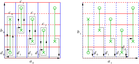
Figure 2. A symplectic basis for $H_{1}(\tilde{T};\mathbb{Z})$.

The relative Maslov grading between two generators (an integer if they are in the same spin^c structure, and a rational number otherwise) can be computed as described in Section 2. Because all the basepoints in the Heegaard diagrams used in this paper are contained in octagonal regions, it is not possible to compute the absolute Maslov gradings or the spectral sequence from $\widehat{\operatorname{HFK}}(\Sigma^{2}(K),\tilde{K})$ to $\widehat{\operatorname{HF}}(\Sigma^{2}(K))$ combinatorially. However, in many instances, the groups $\widehat{\operatorname{HF}}(\Sigma^{2}(K))$, or at least the correction terms $d(\Sigma^{2}(K),\mathfrak{s})$, can be computed via other means [8, 17]. In such cases, it is often possible to pin down the absolute Maslov gradings for $\widehat{\operatorname{HFK}}(\Sigma^{2}(K),\tilde{K})$. Specifically, the relative Maslov $\mathbb{Q}$-grading and the action of $H_{1}(\Sigma^{2}(K))$ on $\operatorname{Spin}^{c}(\Sigma^{2}(K))$ usually provide enough information to match the groups $\widehat{\operatorname{HFK}}(\Sigma^{2}(K),\tilde{K},\mathfrak{s})$ up with the rational numbers $d(\Sigma^{2}(K),\mathfrak{s})$ that are computed via some other means. If there is a spin^c structure $\mathfrak{s}$ in which $\widehat{\operatorname{HFK}}(\Sigma^{2}(K),\tilde{K},\mathfrak{s})$ has rank 1, then the absolute Maslov grading of that group equals the corresponding $d$ invariant, and the rest of the absolute gradings are completely determined.

5. Results

The tables that follow list the ranks for $\widehat{\operatorname{HFK}}(\Sigma^{2}(K),\tilde{K};\mathbb{Z}/2)$ by means of the Poincaré polynomials:

$$p_{\mathfrak{s}}(q,t)=\sum_{i,j}\dim_{\mathbb{Z}/2}\widehat{\operatorname{HFK}}_{j}(\Sigma^{2}(K),\tilde{K},\mathfrak{s},i;\mathbb{Z}/2)t^{i}q^{j}.$$

The Maslov $\mathbb{Q}$-gradings are normalized so that in the canonical spin^c structure $\mathfrak{s}_{0}$, the nonzero elements in Alexander grading $g(K)$ have Maslov grading $g(K)$. For each knot, the first line gives $p_{\mathfrak{s}_{0}}(q,t)$, and each subsequent line gives $p_{\mathfrak{s}}(q,t)$ for a pair of conjugate spin^c structures. We identify spin^c structures with elements of $H_{1}(\Sigma^{2}(K);\mathbb{Z})$, which is either a cyclic group or the sum of two cyclic groups, taking $\mathfrak{s}_{0}$ to $0$. (Of course, the choice of basis for $H_{1}(\Sigma^{2}(K);\mathbb{Z})$ is not canonical.) In each spin^c structure, most of the nonzero groups lie along a single diagonal; the terms corresponding to the groups not on that diagonal are underlined.

These results were computed using a program written in C++ and Mathematica, based on Baldwin and Gillam’s program [1] for computing $\widehat{\operatorname{HFK}}(S^{3},K)$. Most of the grid diagrams were obtained using Marc Culler’s program Gridlink [3]. Using available computer resources, it was possible to compute $\widehat{\operatorname{HFK}}(\Sigma^{2}(K),\tilde{K})$ for all the three-bridge knots with up to eleven crossings and arc index $\leq 9$, and for many knots with arc index 10. (Grigsby [6] has a much more efficient algorithm for computing $\widehat{\operatorname{HFK}}(\Sigma^{2}(K),\tilde{K})$ when $K$ is two-bridge, so we do not list those knots here.)

$$\begin{array}[]{cccl}K&H_{1}(\Sigma^{2}(K);\mathbb{Z})&\mathfrak{s}&\sum_{i,j}\dim_{\mathbb{Z}/2}\widehat{\operatorname{HFK}}_{j}(\Sigma^{2}(K),\tilde{K},\mathfrak{s},i;\mathbb{Z}/2)t^{i}q^{j}\\ \\ 8_{5}&\ \mathbb{Z}/21&0&q^{-3}t^{-3}+3q^{-2}t^{-2}+4q^{-1}t^{-1}+5+4qt+3q^{2}t^{2}+q^{3}t^{3}\\ &&\pm 1&q^{5/21}(q^{-2}t^{-2}+3q^{-1}t^{-1}+3+3qt+q^{2}t^{2})\\ &&\pm 2&q^{20/21}\\ &&\pm 3&q^{8/7}\\ &&\pm 4&q^{17/21}(q^{-1}t^{-1}+1+qt)\\ &&\pm 5&q^{20/21}\\ &&\pm 6&q^{4/7}\\ &&\pm 7&q^{2/3}(q^{-1}t^{-1}+3+qt)\\ &&\pm 8&q^{5/21}(q^{-2}t^{-2}+3q^{-1}t^{-1}+3+3qt+q^{2}t^{2})\\ &&\pm 9&q^{2/7}(q^{-2}t^{-2}+2q^{-1}t^{-1}+3+2qt+q^{2}t^{2})\\ &&\pm 10&q^{17/21}(q^{-1}t^{-1}+1+qt)\\ \\ 8_{10}&\mathbb{Z}/27&0&q^{-3}t^{-3}+3q^{-2}t^{-2}+6q^{-1}t^{-1}+7+6qt+3q^{2}t^{2}+q^{3}t^{3}\\ &&\pm 1&q^{7/27}(q^{-2}t^{-2}+3q^{-1}t^{-1}+5+3qt+q^{2}t^{2})\\ &&\pm 2&q^{1/27}\\ &&\pm 3&q^{1/3}\\ &&\pm 4&q^{4/27}(q^{-1}t^{-1}+1+qt)\\ &&\pm 5&q^{13/27}\\ &&\pm 6&q^{1/3}\\ &&\pm 7&q^{-8/27}(q^{-1}t^{-1}+1+qt)\\ &&\pm 8&q^{-11/27}(q^{-2}t^{-2}+q^{-1}t^{-1}+1+qt+q^{2}t^{2})\\ &&\pm 9&q^{-1}t^{-1}+1+qt\\ &&\pm 10&q^{25/27}\\ &&\pm 11&q^{10/27}(2q^{-1}t^{-1}+3+2qt)\\ &&\pm 12&q^{1/3}(q^{-2}t^{-2}+2q^{-1}t^{-1}+3+2qt+q^{2}t^{2})\\ &&\pm 13&q^{22/27}(q^{-1}t^{-1}+1+qt)\\ \\ 8_{15}&\mathbb{Z}/33&0&3q^{-2}t^{-2}+8q^{-1}t^{-1}+11+8qt+3q^{2}t^{2}\\ &&\pm 1&q^{13/33}(2q^{-1}t^{-1}+3+2qt)\\ &&\pm 2&q^{-14/33}(q^{-2}t^{-2}+q^{-1}t^{-1}+1+qt+q^{2}t^{2})\\ &&\pm 3&q^{6/11}\\ &&\pm 4&q^{10/33}\\ &&\pm 5&q^{-5/33}(q^{-1}t^{-1}+1+qt)\\ &&\pm 6&q^{2/11}\\ &&\pm 7&q^{10/33}\\ &&\pm 8&q^{7/33}(q^{-1}t^{-1}+1+qt)\\ &&\pm 9&q^{10/11}\\ &&\pm 10&q^{13/33}(2q^{-1}t^{-1}+3+2qt)\\ &&\pm 11&q^{2/3}\\ &&\pm 12&q^{-3/11}(q^{-1}t^{-1}+1+qt)\\ &&\pm 13&q^{-14/33}(q^{-2}t^{-2}+q^{-1}t^{-1}+1+qt+q^{2}t^{2})\\ &&\pm 14&q^{7/33}(q^{-1}t^{-1}+1+qt)\\ &&\pm 15&q^{-4/11}(q^{-2}t^{-2}+2q^{-1}t^{-1}+3+2qt+q^{2}t^{2})\\ &&\pm 16&q^{-5/33}(q^{-1}t^{-1}+1+qt)\\ \\ 8_{16}&\mathbb{Z}/35&0&q^{-3}t^{-3}+4q^{-2}t^{-2}+8q^{-1}t^{-1}+9+8qt+4q^{2}t^{2}+q^{3}t^{3}\\ &&\pm 1&q^{16/35}(q^{-1}t^{-1}+1+qt)\\ &&\pm 2&q^{29/35}\\ &&\pm 3&q^{4/35}(q^{-1}t^{-1}+1+qt)\\ &&\pm 4&q^{11/35}(q^{-2}t^{-2}+3q^{-1}t^{-1}+5+3qt+q^{2}t^{2})\\ &&\pm 5&q^{3/7}(q^{-1}t^{-1}+3+qt)\\ &&\pm 6&q^{16/35}(q^{-1}t^{-1}+1+qt)\\ &&\pm 7&q^{2/5}(2q^{-1}t^{-1}+3+2qt)\\ &&\pm 8&q^{9/35}\\ &&\pm 9&q^{1/35}\\ &&\pm 10&q^{5/7}(q^{-1}t^{-1}+3+qt)\\ &&\pm 11&q^{11/35}(q^{-2}t^{-2}+3q^{-1}t^{-1}+5+3qt+q^{2}t^{2})\\ &&\pm 12&q^{29/35}\\ &&\pm 13&q^{9/35}\\ &&\pm 14&q^{3/5}\\ &&\pm 15&q^{6/7}(q^{-1}t^{-1}+1+qt)\\ &&\pm 16&q^{1/35}\\ &&\pm 17&q^{4/35}(q^{-1}t^{-1}+1+qt)\\ \end{array}$$

$$\begin{array}[]{cccl}K&H_{1}(\Sigma^{2}(K);\mathbb{Z})&\mathfrak{s}&\sum_{i,j}\dim_{\mathbb{Z}/2}\widehat{\operatorname{HFK}}_{j}(\Sigma^{2}(K),\tilde{K},\mathfrak{s},i;\mathbb{Z}/2)t^{i}q^{j}\\ \\ 8_{17}&\mathbb{Z}/37&0&q^{-3}t^{-3}+4q^{-2}t^{-2}+8q^{-1}t^{-1}+11+8qt+4q^{2}t^{2}+q^{3}t^{3}\\ &&\pm 1&q^{2/37}\\ &&\pm 2&q^{8/37}(q^{-1}t^{-1}+3+qt)\\ &&\pm 3&q^{18/37}\\ &&\pm 4&q^{-5/37}(q^{-1}t^{-1}+1+qt)\\ &&\pm 5&q^{13/37}(q^{-2}t^{-2}+3q^{-1}t^{-1}+3+3qt+q^{2}t^{2})\\ &&\pm 6&q^{-2/37}\\ &&\pm 7&q^{-13/37}(q^{-2}t^{-2}+3q^{-1}t^{-1}+3+3qt+q^{2}t^{2})\\ &&\pm 8&q^{17/37}(q^{-1}t^{-1}+1+qt)\\ &&\pm 9&q^{14/37}\\ &&\pm 10&q^{-22/37}\\ &&\pm 11&q^{-17/37}(q^{-1}t^{-1}+1+qt)\\ &&\pm 12&q^{-8/37}(q^{-1}t^{-1}+3+qt)\\ &&\pm 13&q^{5/37}(q^{-1}t^{-1}+1+qt)\\ &&\pm 14&q^{22/37}\\ &&\pm 15&q^{6/37}\\ &&\pm 16&q^{-6/37}\\ &&\pm 17&q^{-14/37}\\ &&\pm 18&q^{-18/37}\\ \\ 8_{18}&\mathbb{Z}/3\oplus\mathbb{Z}/15&(0,0)&q^{-3}t^{-3}+5q^{-2}t^{-2}+10q^{-1}t^{-1}+13+10qt+5q^{2}t^{2}+q^{3}t^{3}\\ &&\pm(0,1)&q^{7/15}(q^{-1}t^{-1}+1+qt)\\ &&\pm(0,2)&q^{-2/15}\\ &&\pm(0,3)&q^{1/5}(q^{-1}t^{-1}+1+qt)\\ &&\pm(0,4)&q^{7/15}(q^{-1}t^{-1}+1+qt)\\ &&\pm(0,5)&q^{-2/3}\\ &&\pm(0,6)&q^{-1/5}(q^{-1}t^{-1}+1+qt)\\ &&\pm(0,7)&q^{-2/15}\\ &&\pm(1,0)&q^{-2/3}\\ &&\pm(1,1)&q^{7/15}(q^{-1}t^{-1}+1+qt)\\ &&\pm(1,2)&q^{-7/15}(q^{-1}t^{-1}+1+qt)\\ &&\pm(1,3)&q^{-7/15}(q^{-1}t^{-1}+1+qt)\\ &&\pm(1,4)&q^{7/15}(q^{-1}t^{-1}+1+qt)\\ &&\pm(1,5)&q^{-2/3}\\ &&\pm(1,6)&q^{2/15}\\ &&\pm(1,7)&q^{-2/15}\\ &&\pm(1,8)&q^{-7/15}(q^{-1}t^{-1}+1+qt)\\ &&\pm(1,9)&q^{2/15}\\ &&\pm(1,10)&q^{2/3}\\ &&\pm(1,11)&q^{2/15}\\ &&\pm(1,12)&q^{-7/15}(q^{-1}t^{-1}+1+qt)\\ &&\pm(1,13)&q^{-2/15}\\ &&\pm(1,14)&q^{2/15}\\ \\ 8_{19}&\mathbb{Z}/3&0&q^{-3}t^{-3}+q^{-2}t^{-2}+\underline{q}+q^{2}t^{2}+q^{3}t^{3}\\ &&\pm 1&q^{2/3}(q^{-1}t^{-1}+1+qt)\\ \\ 8_{20}&\mathbb{Z}/9&0&q^{-2}t^{-2}+2q^{-1}t^{-1}+3+2qt+q^{2}t^{2}\\ &&\pm 1&q^{7/9}(q^{-1}t^{-1}+1+qt)\\ &&\pm 2&q^{1/9}(q^{-1}t^{-1}+1+qt)\\ &&\pm 3&1\\ &&\pm 4&q^{4/9}\\ \\ 8_{21}&\mathbb{Z}/15&1&q^{-2}t^{-2}+4q^{-1}t^{-1}+5+4qt+q^{2}t^{2}\\ &&\pm 1&q^{-2/15}(q^{-1}t^{-1}+1+qt)\\ &&\pm 2&q^{7/15}\\ &&\pm 3&q^{-1/5}(q^{-1}t^{-1}+3+qt)\\ &&\pm 4&q^{-2/15}(q^{-1}t^{-1}+1+qt)\\ &&\pm 5&q^{-1/3}\\ &&\pm 6&q^{1/5}\\ &&\pm 7&q^{7/15}\\ \end{array}$$

$$\begin{array}[]{cccl}K&H_{1}(\Sigma^{2}(K);\mathbb{Z})&\mathfrak{s}&\sum_{i,j}\dim_{\mathbb{Z}/2}\widehat{\operatorname{HFK}}_{j}(\Sigma^{2}(K),\tilde{K},\mathfrak{s},i;\mathbb{Z}/2)t^{i}q^{j}\\ \\ 9_{42}&\mathbb{Z}/7&0&q^{-2}t^{-2}+2q^{-1}t^{-1}+2+\underline{q}+2qt+q^{2}t^{2}\\ &&\pm 1&q^{3/7}\\ &&\pm 2&q^{5/7}(q^{-1}t^{-1}+3+qt)\\ &&\pm 3&q^{6/7}(q^{-1}t^{-1}+1+qt)\\ \\ 9_{43}&\mathbb{Z}/13&0&q^{-3}t^{-3}+3q^{-2}t^{-2}+2q^{-1}t^{-1}+1+2qt+3q^{2}t^{2}+q^{3}t^{3}\\ &&\pm 1&q^{10/13}(q^{-1}t^{-1}+3+qt)\\ &&\pm 2&q^{1/13}(q^{-1}t^{-1}+1+qt)\\ &&\pm 3&q^{12/13}\\ &&\pm 4&q^{4/13}(q^{-2}t^{-2}+q^{-1}t^{-1}+1+qt+q^{2}t^{2})\\ &&\pm 5&q^{16/13}\\ &&\pm 6&q^{9/13}(q^{-1}t^{-1}+1+qt)\\ \\ 9_{44}&\mathbb{Z}/17&0&q^{-2}t^{-2}+4q^{-1}t^{-1}+7+4qt+q^{2}t^{2}\\ &&\pm 1&q^{-8/17}\\ &&\pm 2&q^{-15/17}(q^{-1}t^{-1}+1+qt)\\ &&\pm 3&q^{-4/17}\\ &&\pm 4&q^{8/17}\\ &&\pm 5&q^{4/17}\\ &&\pm 6&q^{-16/17}\\ &&\pm 7&q^{-1/17}(q^{-1}t^{-1}+1+qt)\\ &&\pm 8&q^{-2/17}(q^{-1}t^{-1}+3+qt)\\ \\ 9_{45}&\mathbb{Z}/23&0&q^{-2}t^{-2}+6q^{-1}t^{-1}+9+6qt+q^{2}t^{2}\\ &&\pm 1&q^{-8/23}(2q^{-1}t^{-1}+3+2qt)\\ &&\pm 2&q^{-9/23}\\ &&\pm 3&q^{-3/23}(q^{-1}t^{-1}+3+qt)\\ &&\pm 4&q^{-13/23}\\ &&\pm 5&q^{7/23}\\ &&\pm 6&q^{11/23}\\ &&\pm 7&q^{-1/23}\\ &&\pm 8&q^{-6/23}(q^{-1}t^{-1}+1+qt)\\ &&\pm 9&q^{-4/23}(2q^{-1}t^{-1}+3+2qt)\\ &&\pm 10&q^{-18/23}(q^{-1}t^{-1}+1+qt)\\ &&\pm 11&q^{-2/23}(q^{-1}t^{-1}+1+qt)\\ \\ 9_{46}&\mathbb{Z}/3\oplus\mathbb{Z}/3&(0,0)&2q^{-1}t^{-1}+5+2qt\\ &&\pm(0,1)&q^{-2/3}(q^{-1}t^{-1}+3+qt)\\ &&\pm(1,0)&1\\ &&\pm(1,1)&1\\ &&\pm(1,2)&q^{-4/3}\\ \\ 9_{47}&\mathbb{Z}/3\oplus\mathbb{Z}/9&(0,0)&q^{-3}t^{-3}+4q^{-2}t^{-2}+6q^{-1}t^{-1}+5+6qt+4q^{2}t^{2}+q^{3}t^{3}\\ &&\pm(0,1)&q^{-1/9}(q^{-1}t^{-1}+3+qt)\\ &&\pm(0,2)&q^{-4/9}(q^{-1}t^{-1}+1+qt)\\ &&\pm(0,3)&q^{-1}t^{-1}+1+qt\\ &&\pm(0,4)&q^{-7/9}\\ &&\pm(1,0)&q^{-1/3}\\ &&\pm(1,1)&q^{-1/9}(q^{-1}t^{-1}+3+qt)\\ &&\pm(1,2)&q^{-1/9}(q^{-1}t^{-1}+3+qt)\\ &&\pm(1,3)&q^{-1/3}\\ &&\pm(1,4)&q^{-7/9}\\ &&\pm(1,5)&q^{-4/9}(q^{-1}t^{-1}+1+qt)\\ &&\pm(1,6)&q^{-1/3}\\ &&\pm(1,7)&q^{-4/9}(q^{-1}t^{-1}+1+qt)\\ &&\pm(1,8)&q^{-7/9}\\ \end{array}$$

$$\begin{array}[]{cccl}K&H_{1}(\Sigma^{2}(K);\mathbb{Z})&\mathfrak{s}&\sum_{i,j}\dim_{\mathbb{Z}/2}\widehat{\operatorname{HFK}}_{j}(\Sigma^{2}(K),\tilde{K},\mathfrak{s},i;\mathbb{Z}/2)t^{i}q^{j}\\ \\ 9_{48}&\mathbb{Z}/3\oplus\mathbb{Z}/9&(0,0)&q^{-2}t^{-2}+7q^{-1}t^{-1}+11+7qt+q^{2}t^{2}\\ &&\pm(0,1)&q^{-4/9}(q^{-1}t^{-1}+1+qt)\\ &&\pm(0,2)&q^{2/9}(2q^{-1}t^{-1}+3+2qt)\\ &&\pm(0,3)&q^{-1}t^{-1}+1+qt\\ &&\pm(0,4)&q^{-1/9}\\ &&\pm(1,0)&q^{1/3}\\ &&\pm(1,1)&q^{2/9}(2q^{-1}t^{-1}+3+2qt)\\ &&\pm(1,2)&q^{2/9}(2q^{-1}t^{-1}+3+2qt)\\ &&\pm(1,3)&q^{1/3}\\ &&\pm(1,4)&q^{-4/9}(q^{-1}t^{-1}+1+qt)\\ &&\pm(1,5)&q^{-1/9}\\ &&\pm(1,6)&q^{1/3}\\ &&\pm(1,7)&q^{-1/9}\\ &&\pm(1,8)&q^{-4/9}(q^{-1}t^{-1}+1+qt)\\ \\ 9_{49}&\mathbb{Z}/5\oplus\mathbb{Z}/5&(0,0)&3q^{-2}t^{-2}+6q^{-1}t^{-1}+7+6qt+3q^{2}t^{2}\\ &&\pm(0,1)&q^{-2/5}(q^{-2}t^{-2}+q^{-1}t^{-1}+1+qt+q^{2}t^{2})\\ &&\pm(0,2)&q^{2/5}\\ &&\pm(1,0)&q^{-2/5}(q^{-2}t^{-2}+q^{-1}t^{-1}+1+qt+q^{2}t^{2})\\ &&\pm(1,1)&q^{-1/5}(q^{-1}t^{-1}+1+qt)\\ &&\pm(1,2)&q^{1/5}(2q^{-1}t^{-1}+3+2qt)\\ &&\pm(1,3)&q^{1/5}(2q^{-1}t^{-1}+3+2qt)\\ &&\pm(1,4)&q^{-2/5}(q^{-2}t^{-2}+q^{-1}t^{-1}+1+qt+q^{2}t^{2})\\ &&\pm(2,0)&q^{2/5}\\ &&\pm(2,1)&q^{1/5}(2q^{-1}t^{-1}+3+2qt)\\ &&\pm(2,2)&q^{-1/5}(q^{-1}t^{-1}+1+qt)\\ &&\pm(2,3)&q^{2/5}\\ &&\pm(2,4)&q^{-1/5}(q^{-1}t^{-1}+1+qt)\\ \\ 10_{124}&\{0\}&0&q^{-4}t^{-4}+q^{-3}t^{-3}+\underline{t^{-1}+q+q^{2}t}+q^{3}t^{3}+q^{4}t^{4}\\ \\ 10_{128}&\mathbb{Z}/11&0&2q^{-3}t^{-3}+3q^{-2}t^{-2}+q^{-1}t^{-1}+\underline{q}+qt+3q^{2}t^{2}+2q^{3}t^{3}\\ &&\pm 1&q^{8/11}(2q^{-1}t^{-1}+3+2qt)\\ &&\pm 2&q^{10/11}(q^{-1}t^{-1}+1+qt)\\ &&\pm 3&q^{6/11}(q^{-1}t^{-1}+1+qt)\\ &&\pm 4&q^{-4/11}(q^{-2}t^{-2}+q^{-1}t^{-1}+\underline{q}+qt+q^{2}t^{2})\\ &&\pm 5&q^{2/11}(q^{-1}t^{-1}+1+qt)\\ \\ 10_{129}&\mathbb{Z}/25&0&2q^{-2}t^{-2}+6q^{-1}t^{-1}+9+6qt+2q^{2}t^{2}\\ &&\pm 1&q^{-8/25}(q^{-2}t^{-2}+2q^{-1}t^{-1}+3+2qt+q^{2}t^{2})\\ &&\pm 2&q^{-7/25}(q^{-1}t^{-1}+1+qt)\\ &&\pm 3&q^{3/25}(2q^{-1}t^{-1}+3+2qt)\\ &&\pm 4&q^{-3/25}(q^{-1}t^{-1}+1+qt)\\ &&\pm 5&1\\ &&\pm 6&q^{12/25}\\ &&\pm 7&q^{8/25}\\ &&\pm 8&q^{-12/25}\\ &&\pm 9&q^{2/25}(q^{-1}t^{-1}+3+qt)\\ &&\pm 10&1\\ &&\pm 11&q^{7/25}(q^{-1}t^{-1}+1+qt)\\ &&\pm 12&q^{23/25}(q^{-1}t^{-1}+1+qt)\\ \\ 10_{130}&\mathbb{Z}/17&0&2q^{-2}t^{-2}+4q^{-1}t^{-1}+5+4qt+2q^{2}t^{2}\\ &&\pm 1&q^{4/17}(q^{-2}t^{-2}+2q^{-1}t^{-1}+3+2qt+q^{2}t^{2})\\ &&\pm 2&q^{16/17}\\ &&\pm 3&q^{19/17}(q^{-1}t^{-1}+1+qt)\\ &&\pm 4&q^{13/17}(2q^{-1}t^{-1}+3+2qt)\\ &&\pm 5&q^{15/17}(q^{-1}t^{-1}+1+qt)\\ &&\pm 6&q^{8/17}\\ &&\pm 7&q^{9/17}(q^{-1}t^{-1}+1+qt)\\ &&\pm 8&q^{1/17}(q^{-1}t^{-1}+1+qt)\\ \end{array}$$

$$\begin{array}[]{cccl}K&H_{1}(\Sigma^{2}(K);\mathbb{Z})&\mathfrak{s}&\sum_{i,j}\dim_{\mathbb{Z}/2}\widehat{\operatorname{HFK}}_{j}(\Sigma^{2}(K),\tilde{K},\mathfrak{s},i;\mathbb{Z}/2)t^{i}q^{j}\\ \\ 10_{131}&\mathbb{Z}/31&0&2q^{-2}t^{-2}+8q^{-1}t^{-1}+11+8qt+2q^{2}t^{2}\\ &&\pm 1&q^{-18/31}(q^{-1}t^{-1}+1+qt)\\ &&\pm 2&q^{-10/31}(q^{-1}t^{-1}+1+qt)\\ &&\pm 3&q^{-7/31}(q^{-1}t^{-1}+3+qt)\\ &&\pm 4&q^{-9/31}\\ &&\pm 5&q^{15/31}\\ &&\pm 6&q^{3/31}\\ &&\pm 7&q^{-14/31}(q^{-1}t^{-1}+1+qt)\\ &&\pm 8&q^{-5/31}(2q^{-1}t^{-1}+5+2qt)\\ &&\pm 9&q^{-1/31}\\ &&\pm 10&q^{-2/31}(q^{-1}t^{-1}+1+qt)\\ &&\pm 11&q^{-8/31}(q^{-2}t^{-2}+4q^{-1}t^{-1}+5+4qt+q^{2}t^{2})\\ &&\pm 12&q^{-19/31}(q^{-1}t^{-1}+3+qt)\\ &&\pm 13&q^{-4/31}(2q^{-1}t^{-1}+3+2qt)\\ &&\pm 14&q^{-25/31}\\ &&\pm 15&q^{11/31}\\ \\ 10_{132}&\mathbb{Z}/5&0&q^{-2}t^{-2}+(2q^{-1}+\underline{1})t^{-1}+(2+\underline{q})+(2q+\underline{q^{2}})t+q^{2}t^{2}\\ &&\pm 1&q^{2/5}\\ &&\pm 2&q^{3/5}(q^{-1}t^{-1}+1+qt)\\ \\ 10_{133}&\mathbb{Z}/19&0&q^{-2}t^{-2}+5q^{-1}t^{-1}+7+5qt+q^{2}t^{2}\\ &&\pm 1&q^{-3/19}\\ &&\pm 2&q^{-12/19}(q^{-1}t^{-1}+1+qt)\\ &&\pm 3&q^{-8/19}(q^{-1}t^{-1}+1+qt)\\ &&\pm 4&q^{9/19}\\ &&\pm 5&q^{1/19}\\ &&\pm 6&q^{-13/19}(q^{-1}t^{-1}+3+qt)\\ &&\pm 7&q^{5/19}\\ &&\pm 8&q^{-2/19}(2q^{-1}t^{-1}+3+2qt)\\ &&\pm 9&q^{-15/19}\\ \\ 10_{134}&\mathbb{Z}/23&0&2q^{-3}t^{-3}+4q^{-2}t^{-2}+4q^{-1}t^{-1}+3+4qt+4q^{2}t^{2}+2q^{3}t^{3}\\ &&\pm 1&q^{8/23}(q^{-1}t^{-1}+1+qt)\\ &&\pm 2&q^{9/23}(q^{-2}t^{-2}+q^{-1}t^{-1}+1+qt+q^{2}t^{2})\\ &&\pm 3&q^{3/23}(q^{-2}t^{-2}+2q^{-1}t^{-1}+3+2qt+q^{2}t^{2})\\ &&\pm 4&q^{-10/23}(q^{-3}t^{-3}+q^{-2}t^{-2}+\underline{q}+q^{2}t^{2}+q^{3}t^{3})\\ &&\pm 5&q^{16/23}(q^{-1}t^{-1}+1+qt)\\ &&\pm 6&q^{12/23}(q^{-1}t^{-1}+1+qt)\\ &&\pm 7&q^{1/23}(q^{-2}t^{-2}+q^{-1}t^{-1}+1+qt+q^{2}t^{2})\\ &&\pm 8&q^{29/23}\\ &&\pm 9&q^{4/23}(q^{-1}t^{-1}+1+qt)\\ &&\pm 10&q^{18/23}(2q^{-1}t^{-1}+3+2qt)\\ &&\pm 11&q^{25/23}\\ \\ 10_{135}&\mathbb{Z}/37&0&3q^{-2}t^{-2}+9q^{-1}t^{-1}+13+9qt+3q^{2}t^{2}\\ &&\pm 1&q^{14/37}\\ &&\pm 2&q^{-18/37}\\ &&\pm 3&q^{15/37}(2q^{-1}t^{-1}+3+2qt)\\ &&\pm 4&q^{2/37}\\ &&\pm 5&q^{17/37}(q^{-1}t^{-1}+1+qt)\\ &&\pm 6&q^{-14/37}(q^{-2}t^{-2}+2q^{-1}t^{-1}+3+2qt+q^{2}t^{2})\\ &&\pm 7&q^{-17/37}(q^{-1}t^{-1}+1+qt)\\ &&\pm 8&q^{8/37}(q^{-2}t^{-2}+3q^{-1}t^{-1}+5+3qt+q^{2}t^{2})\\ &&\pm 9&q^{-13/37}(q^{-1}t^{-1}+1+qt)\\ &&\pm 10&q^{-6/37}\\ &&\pm 11&q^{29/37}(q^{-1}t^{-1}+1+qt)\\ &&\pm 12&q^{18/37}\\ &&\pm 13&q^{-2/37}\\ &&\pm 14&q^{6/37}(q^{-2}t^{-2}+2q^{-1}t^{-1}+3+2qt+q^{2}t^{2})\\ &&\pm 15&q^{5/37}(2q^{-1}t^{-1}+3+2qt)\\ &&\pm 16&q^{-5/37}(q^{-1}t^{-1}+1+qt)\\ &&\pm 17&q^{13/37}(q^{-1}t^{-1}+1+qt)\\ &&\pm 18&q^{22/37}\\ \\ \end{array}$$

$$\begin{array}[]{cccl}K&H_{1}(\Sigma^{2}(K);\mathbb{Z})&\mathfrak{s}&\sum_{i,j}\dim_{\mathbb{Z}/2}\widehat{\operatorname{HFK}}_{j}(\Sigma^{2}(K),\tilde{K},\mathfrak{s},i;\mathbb{Z}/2)t^{i}q^{j}\\ \\ 10_{136}&\mathbb{Z}/15&1&q^{-2}t^{-2}+4q^{-1}t^{-1}+6+\underline{q}+4qt+q^{2}t^{2}\\ &&\pm 1&q^{7/15}\\ &&\pm 2&q^{13/15}(q^{-1}t^{-1}+3+qt)\\ &&\pm 3&q^{1/5}\\ &&\pm 4&q^{7/15}\\ &&\pm 5&q^{2/3}(q^{-1}t^{-1}+1+qt)\\ &&\pm 6&q^{4/5}(2q^{-1}t^{-1}+3+2qt)\\ &&\pm 7&q^{13/15}(q^{-1}t^{-1}+3+qt)\\ \\ 10_{139}&\mathbb{Z}/3&0&q^{-4}t^{-4}+q^{-3}t^{-3}+\underline{2qt^{-1}+3q+2q^{3}t}+q^{3}t^{3}+q^{4}t^{4}\\ &&\pm 1&q^{5/3}(q^{-2}t^{-2}+q^{-1}t^{-1}+1+qt+q^{2}t^{2})\\ \\ 10_{140}&\mathbb{Z}/9&0&q^{-2}t^{-2}+2q^{-1}t^{-1}+3+2qt+q^{2}t^{2}\\ &&\pm 1&q^{11/9}(q^{-1}t^{-1}+1+qt)\\ &&\pm 2&q^{8/9}\\ &&\pm 3&1\\ &&\pm 4&q^{5/9}(q^{-1}t^{-1}+1+qt)\\ \\ 10_{142}&\mathbb{Z}/15&0&q^{-3}t^{-3}+3q^{-2}t^{-2}+2q^{-1}t^{-1}+1+2qt+3q^{2}t^{2}+2q^{3}t^{3}\\ &&\pm 1&q^{1/15}(q^{-2}t^{-2}+q^{-1}t^{-1}+1+qt+q^{2}t^{2})\\ &&\pm 2&q^{4/15}(q^{-1}t^{-1}+1+qt)\\ &&\pm 3&q^{-2/5}(q^{-3}t^{-3}+q^{-2}t^{-2}+\underline{q}+q^{2}t^{2}+q^{3}t^{3})\\ &&\pm 1&q^{1/15}(q^{-2}t^{-2}+q^{-1}t^{-1}+1+qt+q^{2}t^{2})\\ &&\pm 6&q^{2/3}(2q^{-1}t^{-1}+3+2qt)\\ &&\pm 2&q^{7/5}\\ &&\pm 2&q^{4/15}(q^{-1}t^{-1}+1+qt)\\ \\ 10_{145}&\mathbb{Z}/3&0&q^{-2}t^{-2}+(q^{-1}+\underline{2q})t^{-1}+\underline{q+4q^{2}}+(q+\underline{2q^{3}})t+q^{2}t^{2}\\ &&\pm 1&q^{4/3}(2q^{-1}t^{-1}+3+2qt)\\ \\ 10_{147}&\mathbb{Z}/27&0&2q^{-2}t^{-2}+7q^{-1}t^{-1}+9+7qt+2q^{2}t^{2}\\ &&\pm 1&q^{7/27}(q^{-1}t^{-1}+3+qt)\\ &&\pm 2&q^{1/27}\\ &&\pm 3&q^{1/3}(2q^{-1}t^{-1}+5+2qt)\\ &&\pm 4&q^{4/27}(q^{-2}t^{-2}+3q^{-1}t^{-1}+3+3qt+q^{2}t^{2})\\ &&\pm 5&q^{13/27}\\ &&\pm 6&q^{1/3}\\ &&\pm 7&q^{19/27}(q^{-1}t^{-1}+3+qt)\\ &&\pm 8&q^{16/27}(q^{-1}t^{-1}+1+qt)\\ &&\pm 9&q^{-1}t^{-1}+1+qt\\ &&\pm 10&q^{25/27}\\ &&\pm 11&q^{37/27}\\ &&\pm 12&q^{1/3}\\ &&\pm 13&q^{22/27}(2q^{-1}t^{-1}+3+2qt)\\ \end{array}$$

$$\begin{array}[]{cccl}K&H_{1}(\Sigma^{2}(K);\mathbb{Z})&\mathfrak{s}&\sum_{i,j}\dim_{\mathbb{Z}/2}\widehat{\operatorname{HFK}}_{j}(\Sigma^{2}(K),\tilde{K},\mathfrak{s},i;\mathbb{Z}/2)t^{i}q^{j}\\ \\ 10_{158}&\mathbb{Z}/45&0&q^{-3}t^{-3}+4q^{-2}t^{-2}+10q^{-1}t^{-1}+15+10qt+4q^{2}t^{2}+q^{3}t^{3}\\ &&\pm 1&q^{8/45}(q^{-1}t^{-1}+3+qt)\\ &&\pm 2&q^{-13/45}(q^{-2}t^{-2}+3q^{-1}t^{-1}+3+3qt+q^{2}t^{2})\\ &&\pm 3&q^{-2/5}\\ &&\pm 4&q^{38/45}\\ &&\pm 5&q^{4/9}(q^{-1}t^{-1}+3+qt)\\ &&\pm 6&q^{-2/5}\\ &&\pm 7&q^{-13/45}(q^{-2}t^{-2}+3q^{-1}t^{-1}+3+3qt+q^{2}t^{2})\\ &&\pm 8&q^{17/45}(q^{-2}t^{-2}+3q^{-1}t^{-1}+3+3qt+q^{2}t^{2})\\ &&\pm 9&q^{2/5}(2q^{-1}t^{-1}+5+2qt)\\ &&\pm 10&q^{-2/9}(2q^{-1}t^{-1}+5+2qt)\\ &&\pm 11&q^{-22/45}\\ &&\pm 12&q^{-2/5}\\ &&\pm 13&q^{-2/45}\\ &&\pm 14&q^{38/45}\\ &&\pm 15&q^{-1}t^{-1}+3+qt\\ &&\pm 16&q^{-22/45}\\ &&\pm 17&q^{17/45}(q^{-2}t^{-2}+3q^{-1}t^{-1}+3+3qt+q^{2}t^{2})\\ &&\pm 18&q^{-2/5}\\ &&\pm 19&q^{8/45}(q^{-1}t^{-1}+3+qt)\\ &&\pm 20&q^{1/9}(q^{-1}t^{-1}+1+qt)\\ &&\pm 21&q^{2/5}\\ &&\pm 22&q^{2/45}\\ \\ 10_{160}&\mathbb{Z}/21&0&q^{-3}t^{-3}+4q^{-2}t^{-2}+4q^{-1}t^{-1}+3+4qt+4q^{2}t^{2}+q^{3}t^{3}\\ &&\pm 1&q^{1/21}(q^{-1}t^{-1}+1+qt)\\ &&\pm 2&q^{4/21}(q^{-2}t^{-2}+q^{-1}t^{-1}+1+qt+q^{2}t^{2})\\ &&\pm 3&q^{3/7}(q^{-1}t^{-1}+1+qt)\\ &&\pm 4&q^{16/21}\\ &&\pm 5&q^{4/21}(q^{-2}t^{-2}+q^{-1}t^{-1}+1+qt+q^{2}t^{2})\\ &&\pm 6&q^{5/7}(2q^{-1}t^{-1}+3+2qt)\\ &&\pm 7&q^{4/3}\\ &&\pm 8&q^{1/21}(q^{-1}t^{-1}+1+qt)\\ &&\pm 9&q^{6/7}(q^{-1}t^{-1}+3+qt)\\ &&\pm 10&q^{16/21}\\ \\ 10_{161}&\mathbb{Z}/5&0&q^{-3}t^{-3}+(q^{-2}+\underline{1})t^{-2}+\underline{2qt^{-1}+3q^{2}+2q^{3}t}+(q^{2}+\underline{q^{4}})t^{2}+q^{3}t^{3}\\ &&\pm 1&q^{9/5}(2q^{-1}t^{-1}+3+2qt)\\ &&\pm 2&q^{6/5}(q^{-2}t^{-2}+q^{-1}t^{-1}+1+qt+q^{2}t^{2})\\ \\ 10_{164}&\mathbb{Z}/45&0&3q^{-2}t^{-2}+11q^{-1}t^{-1}+17+11qt+3q^{2}t^{2}\\ &&\pm 1&q^{17/45}(q^{-1}t^{-1}+1+qt)\\ &&\pm 2&q^{-22/45}\\ &&\pm 3&q^{2/5}\\ &&\pm 4&q^{2/45}\\ &&\pm 5&q^{4/9}(q^{-1}t^{-1}+3+qt)\\ &&\pm 6&q^{-2/5}\\ &&\pm 7&q^{-2/45}\\ &&\pm 8&q^{8/45}(q^{-2}t^{-2}+3q^{-1}t^{-1}+5+3qt+q^{2}t^{2})\\ &&\pm 9&q^{-2/5}(q^{-2}t^{-2}+2q^{-1}t^{-1}+3+2qt+q^{2}t^{2})\\ &&\pm 10&q^{-2/9}\\ &&\pm 11&q^{-13/45}(q^{-1}t^{-1}+1+qt)\\ &&\pm 12&q^{2/5}\\ &&\pm 13&q^{38/45}\\ &&\pm 14&q^{2/45}\\ &&\pm 15&q^{-1}t^{-1}+3+qt\\ &&\pm 16&q^{-13/45}(q^{-1}t^{-1}+1+qt)\\ &&\pm 17&q^{8/45}(q^{-2}t^{-2}+3q^{-1}t^{-1}+5+3qt+q^{2}t^{2})\\ &&\pm 18&q^{2/5}\\ &&\pm 19&q^{17/45}(q^{-1}t^{-1}+1+qt)\\ &&\pm 20&q^{1/9}(2q^{-1}t^{-1}+3+2qt)\\ &&\pm 21&q^{-2/5}\\ &&\pm 22&q^{38/45}\\ \end{array}$$

$$\begin{array}[]{cccl}K&H_{1}(\Sigma^{2}(K);\mathbb{Z})&\mathfrak{s}&\sum_{i,j}\dim_{\mathbb{Z}/2}\widehat{\operatorname{HFK}}_{j}(\Sigma^{2}(K),\tilde{K},\mathfrak{s},i;\mathbb{Z}/2)t^{i}q^{j}\\ \\ 11n_{12}&\mathbb{Z}/13&0&q^{-2}t^{-2}+(\underline{q^{-2}}+4q^{-1})t^{-1}+\underline{q^{-1}}+6+(\underline{1}+4q)t+q^{2}t^{2}\\ &&\pm 1&q^{-2/13}\\ &&\pm 2&q^{-8/13}(q^{-1}t^{-1}+3+qt)\\ &&\pm 3&q^{-18/13}\\ &&\pm 4&q^{-6/13}\\ &&\pm 5&q^{-11/13}(2q^{-1}t^{-1}+3+2qt)\\ &&\pm 6&q^{-7/13}(q^{-1}t^{-1}+1+qt)\\ \\ 11n_{19}&\mathbb{Z}/5&0&q^{-3}t^{-3}+2q^{-2}t^{-2}+(q^{-1}+\underline{1})t^{-1}+\underline{q}+(q+\underline{q^{2}})t+2q^{2}t^{2}+q^{3}t^{3}\\ &&\pm 1&q^{4/5}(q^{-2}t^{-2}+q^{-1}t^{-1}+1+qt+q^{2}t^{2})\\ &&\pm 2&q^{6/5}(q^{-1}t^{-1}+3+qt)\\ \\ 11n_{20}&\mathbb{Z}/23&0&2q^{-2}t^{-2}+6q^{-1}t^{-1}+\underline{8+q}+6qt+2q^{2}t^{2}\\ &&\pm 1&q^{17/23}(q^{-1}t^{-1}+3+qt)\\ &&\pm 2&q^{-1/23}\\ &&\pm 3&q^{-8/23}q^{-2}t^{-2}+2q^{-1}t^{-1}+\underline{2+q}+2qt+1q^{2}t^{2}\\ &&\pm 4&q^{19/23}(2q^{-1}t^{-1}+5+2qt)\\ &&\pm 5&q^{11/23}\\ &&\pm 6&q^{14/23}(q^{-1}t^{-1}+1+qt)\\ &&\pm 7&q^{5/23}(q^{-1}t^{-1}+3+qt)\\ &&\pm 8&q^{7/23}\\ &&\pm 9&q^{20/23}(2q^{-1}t^{-1}+3+2qt)\\ &&\pm 10&q^{21/23}(q^{-1}t^{-1}+3+qt)\\ &&\pm 11&q^{10/23}(q^{-1}t^{-1}+1+qt)\\ \\ 11n_{38}&\mathbb{Z}/3&0&q^{-2}t^{-2}+(2q^{-1}+\underline{1})t^{-1}+\underline{2+3q}+(2q+\underline{q^{2}})t+q^{2}t^{2}\\ &&\pm 1&q^{4/3}(q^{-1}t^{-1}+1+qt)\\ \\ 11n_{49}&\{0\}&0&q^{-2}t^{-2}+(\underline{4q^{-3}}+2q^{-1})t^{-1}+\underline{9q^{-2}}+2+(\underline{4q^{-1}}+q)t+q^{2}t^{2}\\ \\ 11n_{95}&\mathbb{Z}/33&0&q^{-3}t^{-3}+5q^{-2}t^{-2}+7q^{-1}t^{-1}+7+7qt+5q^{2}t^{2}+q^{3}t^{3}\\ &&\pm 1&q^{-13/33}(q^{-1}t^{-1}+1+qt)\\ &&\pm 2&q^{14/33}\\ &&\pm 3&q^{5/11}(q^{-1}t^{-1}+1+qt)\\ &&\pm 4&q^{-10/33}(q^{-2}t^{-2}+q^{-1}t^{-1}+1+qt+q^{2}t^{2})\\ &&\pm 5&q^{5/33}(2q^{-1}t^{-1}+3+2qt)\\ &&\pm 6&q^{-2/11}(q^{-2}t^{-2}+q^{-1}t^{-1}+1+qt+q^{2}t^{2})\\ &&\pm 7&q^{-10/33}(q^{-2}t^{-2}+q^{-1}t^{-1}+1+qt+q^{2}t^{2})\\ &&\pm 8&q^{26/33}\\ &&\pm 9&q^{1/11}(q^{-1}t^{-1}+1+qt)\\ &&\pm 10&q^{-13/33}(q^{-1}t^{-1}+1+qt)\\ &&\pm 11&q^{1/3}(q^{-1}t^{-1}+1+qt)\\ &&\pm 12&q^{3/11}(2q^{-1}t^{-1}+3+2qt)\\ &&\pm 13&q^{14/33}\\ &&\pm 14&q^{26/33}\\ &&\pm 15&q^{4/11}(q^{-1}t^{-1}+3+qt)\\ &&\pm 16&q^{5/33}(2q^{-1}t^{-1}+3+2qt)\\ \\ 11n_{102}&\mathbb{Z}/3&0&q^{-2}t^{-2}+(5q^{-1}+\underline{2q})t^{-1}+7+\underline{4q^{2}}+(5q+\underline{2q^{3}})t+q^{2}t^{2}\\ &&\pm 1&q^{1/3}(2q^{-1}t^{-1}+5+2qt)\\ \\ 11n_{116}&\{0\}&0&q^{-2}t^{-2}+(\underline{4q^{-3}}+2q^{-1})t^{-1}+\underline{9q^{-2}}+2+(\underline{4q^{-1}}+q)t+q^{2}t^{2}\\ \end{array}$$

$$\begin{array}[]{cccl}K&H_{1}(\Sigma^{2}(K);\mathbb{Z})&\mathfrak{s}&\sum_{i,j}\dim_{\mathbb{Z}/2}\widehat{\operatorname{HFK}}_{j}(\Sigma^{2}(K),\tilde{K},\mathfrak{s},i;\mathbb{Z}/2)t^{i}q^{j}\\ \\ 11n_{117}&\mathbb{Z}/35&0&3q^{-2}t^{-2}+9q^{-1}t^{-1}+11+9qt+3q^{2}t^{2}\\ &&\pm 1&q^{9/35}(2q^{-1}t^{-1}+5+2qt)\\ &&\pm 2&q^{1/35}\\ &&\pm 3&q^{11/35}(q^{-1}t^{-1}+3+qt)\\ &&\pm 4&q^{4/35}(q^{-2}t^{-2}+3q^{-1}t^{-1}+3+3qt+q^{2}t^{2})\\ &&\pm 5&q^{3/7}(q^{-1}t^{-1}+3+qt)\\ &&\pm 6&q^{9/35}(2q^{-1}t^{-1}+5+2qt)\\ &&\pm 7&q^{-2/5}(q^{-2}t^{-2}+2q^{-1}t^{-1}+2+\underline{q}+2qt+q^{2}t^{2})\\ &&\pm 8&q^{16/35}(q^{-1}t^{-1}+1+qt)\\ &&\pm 9&q^{29/35}\\ &&\pm 10&q^{5/7}(2q^{-1}t^{-1}+5+2qt)\\ &&\pm 11&q^{4/35}(q^{-2}t^{-2}+3q^{-1}t^{-1}+3+3qt+q^{2}t^{2})\\ &&\pm 12&q^{1/355}\\ &&\pm 13&q^{16/35}(q^{-1}t^{-1}+1+qt)\\ &&\pm 14&q^{7/5}\\ &&\pm 15&q^{6/7}(2q^{-1}t^{-1}+3+2qt)\\ &&\pm 16&q^{29/35}\\ &&\pm 17&q^{11/35}(q^{-1}t^{-1}+3+qt)\\ \\ 11n_{118}&\mathbb{Z}/21&0&q^{-3}t^{-3}+4q^{-2}t^{-2}+4q^{-1}t^{-1}+3+4qt+4q^{2}t^{2}+q^{3}t^{3}\\ &&\pm 1&q^{5/21}(q^{-1}t^{-1}+1+qt)\\ &&\pm 2&q^{20/21}\\ &&\pm 3&q^{1/7}(2q^{-1}t^{-1}+3+2qt)\\ &&\pm 4&q^{-4/21}(q^{-2}t^{-2}+q^{-1}t^{-1}+1+qt+q^{2}t^{2})\\ &&\pm 5&q^{20/21}\\ &&\pm 6&q^{4/7}\\ &&\pm 7&q^{-1/3}(q^{-1}t^{-1}+1+qt)\\ &&\pm 8&q^{5/21}(q^{-1}t^{-1}+1+qt)\\ &&\pm 9&q^{2/7}(q^{-1}t^{-1}+3+qt)\\ &&\pm 10&q^{-4/21}(q^{-2}t^{-2}+q^{-1}t^{-1}+1+qt+q^{2}t^{2})\\ \\ 11n_{122}&\mathbb{Z}/27&0&2q^{-2}t^{-2}+7q^{-1}t^{-1}+9+2qt+2q^{2}t^{2}\\ &&\pm 1&q^{13/27}\\ &&\pm 2&q^{-2/27}(2q^{-1}t^{-1}+3+2qt)\\ &&\pm 3&q^{1/3}(2q^{-1}t^{-1}+5+2qt)\\ &&\pm 4&q^{-8/27}(q^{-1}t^{-1}+1+qt)\\ &&\pm 5&q^{1/27}\\ &&\pm 6&q^{1/3}\\ &&\pm 7&q^{-11/27}\\ &&\pm 8&q^{-5/27}(q^{-1}t^{-1}+3+qt)\\ &&\pm 9&q^{-1}t^{-1}+1+qt\\ &&\pm 10&q^{-23/27}\\ &&\pm 11&q^{-20/27}(q^{-2}t^{-2}+3q^{-1}t^{-1}+3+3qt+q^{2}t^{2})\\ &&\pm 12&q^{1/3}\\ &&\pm 13&q^{-17/27}(q^{-1}t^{-1}+3+qt)\\ \\ 11n_{138}&\mathbb{Z}/15&0&2q^{-2}t^{-2}+4q^{-1}t^{-1}+(\underline{q^{-1}}+4)+4qt+2q^{2}t^{2}\\ &&\pm 1&q^{-7/15}\\ &&\pm 2&q^{-13/15}(q^{-1}t^{-1}+3+qt)\\ &&\pm 3&q^{-1/5}((q^{-2}+2q^{-1})t^{-1}+(q^{-1}+4)+(1+2q)t)\\ &&\pm 4&q^{-7/15}\\ &&\pm 5&q^{-2/3}(q^{-2}t^{-2}+3q^{-1}t^{-1}+3+3qt+q^{2}t^{2})\\ &&\pm 6&q^{-9/5}\\ &&\pm 7&q^{-13/15}(q^{-1}t^{-1}+3+qt)\\ \\ 11n_{139}&\mathbb{Z}/9&0&2q^{-1}t^{-1}+5+2qt\\ &&\pm 1&q^{-4/9}\\ &&\pm 2&q^{-16/9}\\ &&\pm 3&1\\ &&\pm 4&q^{-10/9}(q^{-1}t^{-1}+3+qt)\\ \end{array}$$

$$\begin{array}[]{cccl}K&H_{1}(\Sigma^{2}(K);\mathbb{Z})&\mathfrak{s}&\sum_{i,j}\dim_{\mathbb{Z}/2}\widehat{\operatorname{HFK}}_{j}(\Sigma^{2}(K),\tilde{K},\mathfrak{s},i;\mathbb{Z}/2)t^{i}q^{j}\\ \\ 11n_{141}&\mathbb{Z}/21&0&5q^{-1}t^{-1}+11+5qt\\ &&\pm 1&q^{-10/21}\\ &&\pm 2&q^{2/21}(2q^{-1}t^{-1}+5+2qt)\\ &&\pm 3&q^{-2/7}(2q^{-1}t^{-1}+5+2qt)\\ &&\pm 4&q^{8/21}(q^{-1}t^{-1}+3+qt)\\ &&\pm 5&q^{2/21}(2q^{-1}t^{-1}+5+2qt)\\ &&\pm 6&q^{6/7}\\ &&\pm 7&q^{2/3}(2q^{-1}t^{-1}+5+2qt)\\ &&\pm 8&q^{-10/21}\\ &&\pm 9&q^{10/7}\\ &&\pm 10&q^{8/21}(q^{-1}t^{-1}+3+qt)\\ \\ 11n_{142}&\mathbb{Z}/33&0&q^{-2}t^{-2}+8q^{-1}t^{-1}+15+8qt+q^{2}t^{2}\\ &&\pm 1&q^{2/33}(q^{-1}t^{-1}+3+qt)\\ &&\pm 2&q^{8/33}(2q^{-1}t^{-1}+5+2qt)\\ &&\pm 3&q^{6/11}(q^{-1}t^{-1}+3+qt)\\ &&\pm 4&q^{32/33}\\ &&\pm 5&q^{-16/33}\\ &&\pm 6&q^{2/11}(q^{-1}t^{-1}+3+qt)\\ &&\pm 7&q^{32/33}\\ &&\pm 8&q^{-4/33}\\ &&\pm 9&q^{10/11}(q^{-1}t^{-1}+3+qt)\\ &&\pm 10&q^{2/33}(q^{-1}t^{-1}+3+qt)\\ &&\pm 11&q^{4/3}\\ &&\pm 12&q^{8/11}(2q^{-1}t^{-1}+5+2qt)\\ &&\pm 13&q^{8/33}(2q^{-1}t^{-1}+5+2qt)\\ &&\pm 14&q^{-4/33}\\ &&\pm 15&q^{-4/11}(2q^{-1}t^{-1}+5+2qt)\\ &&\pm 16&q^{-16/33}\\ \\ 11n_{143}&\mathbb{Z}/9&0&q^{-3}t^{-3}+(\underline{q^{-4}}+3q^{-2})t^{-2}+(\underline{2q^{-3}}+3q^{-1})t^{-1}+(\underline{2q^{-2}}+3)\\ &&&\quad+(\underline{2q^{-1}}+3q)t+(\underline{1}+3q^{2})t^{2}+q^{3}t^{3}\\ &&\pm 1&q^{-10/9}((q^{-1}+1)t^{-1}+(2+q)+(1+q^{2})t)\\ &&\pm 2&q^{-4/9}\\ &&\pm 3&1\\ &&\pm 4&q^{-7/9}(q^{-2}t^{-2}+3q^{-1}t^{-1}+3+3qt+q^{2}t^{2})\\ \\ 11n_{145}&\mathbb{Z}/9&0&q^{-3}t^{-3}+(2q^{-2}+\underline{1})t^{-2}+(q^{-1}+\underline{4q})t^{-1}+\underline{7q^{2}}+(q+\underline{4q^{3}})t\\ &&&\quad+(2q^{2}+\underline{t^{4}})t^{2}+q^{3}t^{3}\\ &&\pm 1&q^{10/9}(q^{-2}t^{-2}+3q^{-1}t^{-1}+5+3qt+q^{2}t^{2})\\ &&\pm 2&q^{22/9}\\ &&\pm 3&q^{2}\\ &&\pm 4&q^{16/9}(q^{-2}t^{-2}+3q^{-1}t^{-1}+5+3qt+q^{2}t^{2})\\ \end{array}$$

6. Observations

Grigsby [5] showed that when $K\subset S^{3}$ is a two-bridge knot, the Heegaard Floer knot homology of $\tilde{K}\subset\Sigma^{2}(K)$ in the canonical spin^c structure is isomorphic as a bigraded $\mathbb{Z}/2$-vector space to that of $K\subset S^{3}$: i.e., $\widehat{\operatorname{HFK}}(\Sigma^{2}(K),\tilde{K},\mathfrak{s}_{0})\cong\widehat{\operatorname{HFK}}(S^{3},K)$, up to an overall shift in the Maslov grading. Our results suggest that the same is true for a wider class for knots. Specifically, we say that $\widehat{\operatorname{HFK}}(S^{3},K)$ is perfect if it is supported along a single diagonal, i.e., there exists a constant $C$ such that $\widehat{\operatorname{HFK}}_{j}(S^{3},K,i)=0$ when $j-i\neq C$. We conjecture:

Conjecture 6.1.

Let $K\subset S^{3}$ be a knot such that $\widehat{\operatorname{HFK}}(S^{3},K)$ is supported along a single diagonal, i.e., Then $\widehat{\operatorname{HFK}}(\Sigma^{2}(K),\tilde{K},\mathfrak{s}_{0})\cong\widehat{\operatorname{HFK}}(S^{3},K)$ as bigraded groups, up to a possible shift in the absolute Maslov grading.

It is well-known [15, 19] that $\widehat{\operatorname{HFK}}(S^{3},K)$ is perfect whenever $K$ is alternating (and hence for all two-bridge knots). More generally, let $\mathcal{Q}$ be the smallest set of link types such that:

• The unknot is in $\mathcal{Q}$.

• Suppose $L$ admits a projection such that the two resolutions at some crossing, $L_{0}$ and $L_{1}$, are both in $\mathcal{Q}$ and satisfy $\det(L_{0})+\det(L_{1})=\det(L)$. Then $L$ is in $\mathcal{Q}$.

The links in $\mathcal{Q}$ are called quasi-alternating; for instance, any alternating link is quasi-alternating. Manolescu and Ozsváth [11] have shown that whenever $L$ is quasi-alternating, both $\widehat{\operatorname{HFK}}(S^{3},L)$ and the Khovanov homology of $L$ are perfect. (Additionally, Ozsváth and Szabó [16] have shown that the branched double cover of any quasi-alternating link $L$ is an L-space, meaning that $\widehat{\operatorname{HF}}(\Sigma^{2}(L),\mathfrak{s})$ has rank 1 in each spin^c structure.) Conjecture 6.1 would then imply that $\widehat{\operatorname{HFK}}(\Sigma^{2}(K),\tilde{K},\mathfrak{s}_{0})$ is perfect whenever $K$ is quasi-alternating.

One can also ask under what conditions $\widehat{\operatorname{HFK}}(\Sigma^{2}(K),\tilde{K},\mathfrak{s})$ is perfect when $\mathfrak{s}\neq\mathfrak{s}_{0}$. The knots $10_{134}$ and $11n_{117}$ have the property that both $\widehat{\operatorname{HFK}}(S^{3},K)$ and $\widehat{\operatorname{HFK}}(\Sigma^{2}(K),\tilde{K},\mathfrak{s}_{0})$ are perfect and isomorphic, but there is a spin^c structure $\mathfrak{s}$ in which $\widehat{\operatorname{HFK}}(S^{2}(K),\tilde{K},\mathfrak{s})$ is not perfect. It is not known, however, whether these knots are quasi-alternating.

On the other hand, when $\widehat{\operatorname{HFK}}(S^{3},K)$ is not perfect, the isomorphism between $\widehat{\operatorname{HFK}}(S^{3},K)$ and $\widehat{\operatorname{HFK}}(\Sigma^{2}(K),\tilde{K},\mathfrak{s}_{0})$ fails. A few patterns are worth mentioning. If $\widehat{\operatorname{HFK}}(S^{3},K,g)$ (where $g=g(K)$) is supported in a single Maslov grading $g+c$, define the main diagonal of $\widehat{\operatorname{HFK}}(S^{3},K)$ as the groups $\widehat{\operatorname{HFK}}_{i+c}(S^{3},K,i)$. (This assumption fails when the rank of $\Delta_{K}$ is less than twice $g(K)$, for instance.) In every example considered here, the remaining nonzero groups lie either all above $(M>A+c)$ or all below $(M<A+c)$ the main diagonal. (See [1] for the values of $\widehat{\operatorname{HFK}}(S^{3},K)$ for all non-alternating knots with $\leq 12$ crossings.)

In most of our examples, the main diagonal of $\widehat{\operatorname{HFK}}(\Sigma^{2}(K),\tilde{K},\mathfrak{s}_{0})$ is isomorphic to that of $\widehat{\operatorname{HFK}}(S^{3},K)$, while the Maslov gradings of the off-diagonal groups may be shifted by an overall constant. That constant is sometimes odd, implying that the Maslov $\mathbb{Z}/2$-gradings need not be the same. For instance, when $K$ is the knot $10_{161}$, the off-diagonal groups are shifted by three. However, there are also instances where the main diagonals of $\widehat{\operatorname{HFK}}(S^{3},K)$ and $\widehat{\operatorname{HFK}}(\Sigma^{2}(K),\tilde{K},\mathfrak{s}_{0})$ are not isomorphic. When $K=10_{145}$, the matrices of the ranks of $\widehat{\operatorname{HFK}}_{j}(S^{3},K,i)$ and $\widehat{\operatorname{HFK}}_{j}(\Sigma^{2}(K),\tilde{K},i))$ are, respectively,

$$\begin{pmatrix}0&0&0&0&\bm{1}\\ 0&0&0&\bm{1}&0\\ 0&0&\bm{1}&2&0\\ 0&\bm{1}&4&0&0\\ \bm{1}&2&0&0&0\\ \end{pmatrix}\text{ and }\begin{pmatrix}0&0&0&2&0\\ 0&0&4&0&\bm{1}\\ 0&2&1&\bm{1}&0\\ 0&0&\bm{0}&0&0\\ 0&\bm{1}&0&0&0\\ \bm{1}&0&0&0&0\\ \end{pmatrix}$$

(where the Alexander grading is on the horizontal axis, the Maslov grading is on the vertical axis, and the main diagonal is shown in bold). Here, one of the groups on the main diagonal in $\widehat{\operatorname{HFK}}(S^{3},K)$ is shifted upward by one. In this case, the total rank in each Alexander grading is still the same, but there are also instances where that statement fails to hold. For the knots $11n_{49}$ and $11n_{116}$, which have determinant 1 and identical Heegaard Floer homology both downstairs and upstairs, the ranks of $\widehat{\operatorname{HFK}}_{j}(S^{3},K,i)$ and $\widehat{\operatorname{HFK}}_{j}(\Sigma^{2}(K),\tilde{K},\mathfrak{s}_{0},i)$ (in the unique spin^c structure) are given by

$$\begin{pmatrix}0&0&0&2&\bm{1}\\ 0&0&5&\bm{2}&0\\ 0&2&\bm{2}&0&0\\ 0&\bm{2}&0&0&0\\ \bm{1}&0&0&0&0\\ \end{pmatrix}\text{ and }\begin{pmatrix}0&0&0&0&\bm{1}\\ 0&0&0&\bm{2}&0\\ 0&0&\bm{2}&0&0\\ 0&\bm{2}&0&4&0\\ \bm{1}&0&9&0&0\\ 0&4&0&0&0\\ \end{pmatrix}.$$

Another example in which the total ranks of $\widehat{\operatorname{HFK}}(S^{3},K)$ and $\widehat{\operatorname{HFK}}(\Sigma^{2}(K),\tilde{K},\mathfrak{s}_{0})$ are different is the knot $11n_{102}$, for which the ranks are

$$\begin{pmatrix}0&0&0&2&\bm{1}\\ 0&0&4&\bm{3}&0\\ 0&2&\bm{3}&0&0\\ 0&\bm{3}&0&0&0\\ \bm{1}&0&0&0&0\\ \end{pmatrix}\text{ and }\begin{pmatrix}0&0&0&2&0\\ 0&0&4&0&\bm{1}\\ 0&2&0&\bm{5}&0\\ 0&0&\bm{7}&0&0\\ 0&\bm{5}&0&0&0\\ \bm{1}&0&0&0&0\\ \end{pmatrix}.$$

Finally, note that the pretzel knots $8_{20}=P(3,-3,2)$ and $10_{140}=P(4,3,-3)$ have identical knot Floer homology but can be distinguished by $\widehat{\operatorname{HFK}}(\Sigma^{2}(K),\tilde{K})$. The relative Maslov gradings between spin^c structures are necessary in this case. For another such example, see [5].

References

- [1] J. A. Baldwin and W. D. Gillam, Computations of Heegaard Floer knot homology, preprint, math/0610167.
- [2] R. H. Fox, A Quick Trip Through Knot Theory, Topology of 3-Manifolds (1962), 120–167.
-
[3]
M. Culler, Gridlink: a tool for knot theorists.
www.math.uic.edu/~culler/gridlink/. - [4] C. McA. Gordon, Some aspects of classical knot theory, Knot Theory: Proceedings, Plans-Sur-Bex, Switzerland, Lecture Notes in Mathematics 685 (1978), 1–60.
- [5] J. E. Grigsby, Knot Floer homology in cyclic branched covers, Algebr. Geom. Topol. 6 (2006), 1355 1398 (electronic), math/0507498.
- [6] J. E. Grigsby, Combinatorial description of knot Floer homology of cyclic branched covers, math/0610238.
- [7] J. E. Grigsby, D. Ruberman, and S. Strle, Knot concordance and Heegaard Floer homology invariants in branched covers, preprint, math/0701460.
- [8] S. Jabuka and S. Naik, Order in the concordance group and Heegaard Floer homology, Geom. Topol. 11 (2007), 979–994.
- [9] D. A. Lee and R. Lipshitz, Covering spaces and -gradings on Heegaard Floer homology, preprint, math/0608001.
- [10] R. Lipshitz, A cylindrical reformulation of Heegaard Floer homology, Geom. Topol. 10 (2006), 955–1097, math/0502404.
- [11] C. Manolescu and P. Ozsáth, On the Khovanov and knot Floer homologies of quasi-alternating links, preprint, math/0708.3249v1.
- [12] C. Manolescu, P. Ozsváth, and S. Sarkar, A combinatorial description of knot Floer homology, preprint, math/0607691.
- [13] C. Manolescu, P. Ozsváth, Z. Szabó, and D. Thurston. On combinatorial link Floer homology, preprint, math/0610559.
- [14] P. S. Ozsváth and Z. Szabó. Holomorphic disks and knot invariants, Adv. Math. 186 (2004), 58–116.
- [15] P. S. Ozsváth and Z. Szabó. Heegaard Floer homology and alternating knots, Geom. Topol. 7 (2003), 225 -254.
- [16] P. S. Ozsváth and Z. Szabó. On the Heegaard Floer homology of branched double-covers, Adv. Math. 194 (2005), 1 -33.
- [17] P. S. Ozsváth and Z. Szabó. Knots with unknotting number one and Heegaard Floer homology, Topol. 44 (2005), 705 -745.
- [18] J. A. Rasmussen, Floer homology and knot complements, Ph.D. thesis, Harvard University (2003), math/0306378.
- [19] J. A. Rasmussen, Floer homology of surgeries on two-bridge knots, Algebr. Geom. Topol. 2 (2002), 757-789.
- [20] D. Rolfsen, Knots and Links, 3rd ed., AMS Chelsea, 1990.
- [21] S. Sarkar and J. Wang, A combinatorial description of some Heegaard Floer homologies, preprint, math/0607777.
- [22] V. Turaev, Torsion invariants of spinc structures on 3-manifolds, Math. Res. Lett. 4 (1997), 679–695.