Magnetic fields and accretion flows on the classical T Tauri star V2129 Oph

Abstract

From observations collected with the ESPaDOnS spectropolarimeter, we report the discovery of magnetic fields at the surface of the mildly accreting classical T Tauri star (cTTS) V2129 Oph. Zeeman signatures are detected, both in photospheric lines and in the emission lines formed at the base of the accretion funnels linking the disc to the protostar, and monitored over the whole rotation cycle of V2129 Oph. We observe that rotational modulation dominates the temporal variations of both unpolarised and circularly polarised line profiles.

We reconstruct the large-scale magnetic topology at the surface of V2129 Oph from both sets of Zeeman signatures simultaneously. We find it to be rather complex, with a dominant octupolar component and a weak dipole of strengths 1.2 and 0.35 kG respectively, both slightly tilted with respect to the rotation axis. The large-scale field is anchored in a pair of 2 kG unipolar radial field spots located at high latitudes and coinciding with cool dark polar spots at photospheric level. This large-scale field geometry is unusually complex compared to those of non-accreting cool active subgiants with moderate rotation rates.

As an illustration, we provide a first attempt at modelling the magnetospheric topology and accretion funnels of V2129 Oph using field extrapolation. We find that the magnetosphere of V2129 Oph must extend to about 7 $R_{\star}$ to ensure that the footpoints of accretion funnels coincide with the high-latitude accretion spots on the stellar surface. It suggests that the stellar magnetic field succeeds in coupling to the accretion disc as far out as the corotation radius, and could possibly explain the slow rotation of V2129 Oph. The magnetospheric geometry we derive qualitatively reproduces the modulation of Balmer lines and produces X-ray coronal fluxes typical of those observed in cTTSs.

1 Introduction

T Tauri stars (TTSs) are young low-mass stars that have emerged from their natal molecular cloud core. Among them, classical TTSs (cTTSs) are those still surrounded by accretion discs. CTTSs are strongly magnetic; their fields are thought to be responsible for disrupting the central regions of their accretion discs and for channelling the disc material towards the stellar surface along discrete accretion funnels. This magnetically-channelled accretion can determine the angular momentum evolution of protostars (e.g., Königl, 1991; Shu et al., 1994; Cameron & Campbell, 1993; Romanova et al., 2004) as well as their internal structure. Studying magnetospheric accretion processes of cTTSs through both observations and simulations is thus crucial for our understanding of stellar formation.

The Zeeman broadening of unpolarised spectral lines (e.g., Johns-Krull et al., 1999; Yang et al., 2005), has been very successful at determining mean surface magnetic field strengths on cTTSs, even for complex field topologies, but is rather insensitive to the large-scale structure of the field. Spectropolarimetric techniques, aimed at detecting polarised Zeeman signatures in spectral lines, are sensitive to the vector properties of the magnetic field but encounter difficulties in reconstructing highly-complex multipolar field structures. Until now, circular spectropolarimetry has been used, for cTTSs, to detect and estimate magnetic fields in accretion funnels of cTTSs (Johns-Krull et al., 1999; Valenti & Johns-Krull, 2004), but not the photospheric fields (e.g., Valenti & Johns-Krull, 2004; Daou et al., 2006).

Here we report a new study of the cTTS V2129 Oph (SR 9, AS 207A, GY 319, ROX 29, HBC 264), the brightest TTS in the $\rho$ Oph cloud, using ESPaDOnS, the new generation spectropolarimeter recently installed at the 3.6-m Canada–France–Hawaii Telescope (CFHT). After briefly reviewing the fundamental parameters of V2129 Oph (Sec. 2), we present our observations (Sec. 3) and describe the shape and rotational modulation of the Zeeman signatures detected in both photospheric and emission lines (Sec. 4). Using tomographic techniques, we model the distribution of active regions, accretion spots and magnetic fields at the surface of V2129 Oph (Secs. 5 & 6). As an illustration, we provide a first attempt at modelling the magnetosphere and accretion funnels of V2129 Oph ((Sec. 7). We finally discuss the implications of our results for stellar formation (Sec. 8).

2 The cTTS V2129 Oph

Several estimates of the photospheric temperature $T_{\rm eff}$ of V2129 Oph are available in the literature. Bouvier (1990) and Bouvier & Appenzeller (1992) initially suggested that $\hbox{$T_{\rm eff}$}\simeq 4200$ K. Padgett (1996) and Eisner et al. (2005) proposed higher temperatures (4650 and 4400 K respectively) while Geoffray & Monin (2001) and Doppmann et al. (2003) concluded that the star is actually cooler (4000 and 3400 K respectively). These differences probably arise because the spectral energy distribution includes a strong infrared contribution from the accretion disc (Eisner et al., 2005) and, to a lesser extent, from its companion star. The photometric colours of V2129 Oph are, moreover, affected by interstellar reddening, making photometric temperature estimates slightly unreliable. The spectroscopic measurements by Padgett (1996) and Bouvier & Appenzeller (1992) appear safest; we thus choose 4500 K as the most likely estimate, with a typical error bar of about 200 K.

From this temperature estimate, and given the $B-V$, $V-R_{\rm c}$ and $V-I_{\rm c}$ photometric colours of V2129 Oph (respectively equal to 1.25, 0.80 and 1.60, Bouvier 1990), we infer from Kurucz synthetic colours (including interstellar reddening, Kurucz 1993) that the $B-V$ colour excess $E(B-V)\simeq 0.2$ (i.e.  that the interstellar extinction $A_{V}\simeq 0.6$) and that the bolometric correction (including interstellar extinction) is $-1.3$. Although V2129 Oph was too faint to be observed with Hipparcos (and thus to have its parallax estimated accurately), its membership of the $\rho$ Oph dark cloud indicates that its distance is about $140\pm 10$ pc (Bontemps et al., 2001).

Bouvier (1990) and Schevchenko & Herbst (1998) find that the maximum brightness of V2129 Oph (at minimum spot coverage) is about 11.20; its unspotted $V$ magnitude is thus $11.0\pm 0.2$, given that active stars usually feature as much as 20% spot coverage even at brightness maximum (e.g., Donati et al., 2003). From this, we obtain that the bolometric magnitude of V2129 Oph is $4.0\pm 0.25$, i.e. that its logarithmic luminosity (with respect to the Sun) is $0.3\pm 0.1$. Given the assumed $T_{\rm eff}$, we derive that V2129 Oph has a radius of $\hbox{$R_{\star}$}=2.4\pm 0.3$ ${\rm R}_{\odot}$. In Sec. 5 we measure the projected equatorial rotation velocity to be $\hbox{$v\sin i$}=14.5\pm 0.3$ km s^-1, where $i$ is the angle between the rotation axis and the line of sight. This agrees well with published estimates of $15.2\pm 0.9$ km s^-1  and $15.8\pm 1.5$ km s^-1 by Eisner et al. 2005 and Bouvier 1990 respectively. From $v\sin i$ and the rotation period of 6.53 d (Schevchenko & Herbst, 1998), we obtain that $\hbox{$R_{\star}$}\sin i=1.87\pm 0.04$ ${\rm R}_{\odot}$. We infer $i\simeq 50\hbox{${}^{\circ}$}$, in good agreement with the value of 45^∘ derived from tomographic modelling of our data (see Sec. 5).

Fitting the evolutionary models of Siess et al. (2000) to these parameters, we infer that V2129 Oph is a $1.35\pm 0.15$ ${\rm M}_{\odot}$ star with an age of about 2 Myr and is no longer fully convective, with a small radiative core of mass $\simeq 0.1$ $M_{\star}$ and radius $\simeq 0.2$ $R_{\star}$.

From the equivalent width of the 866 nm Ca ii line emission core (about 0.05 nm, see Sec. 4, implying a line emission flux of $10^{-6}$ erg s^-1 cm^-2), we obtain that the mass-accretion rate $\dot{M}$ of V2129 Oph is about $4\times 10^{-9}$ ${\rm M}_{\odot}$ yr^-1  (Mohanty et al., 2005). Eisner et al. (2005) suggests that $\dot{M}$ is significantly larger, about $3\times 10^{-8}$ ${\rm M}_{\odot}$ yr^-1. We assume here that $\hbox{$\dot{M}$}\simeq 10^{-8}$ ${\rm M}_{\odot}$ yr^-1, i.e., a conservative compromise between both estimates and a typical value for a mildly accreting cTTS.

Rotational cycles $E$ are computed according to the ephemeris:

$$\mbox{HJD}=2453540.0+6.53E,$$ (1)

where the rotation period is that determined by Schevchenko & Herbst (1998).

Table 1: Journal of observations. Columns 1–4 sequentially list the UT date, the heliocentric Julian date and UT time (both at mid-exposure), and the peak signal to noise ratio (per 2.6 km s^-1 velocity bin) of each observation. Column 5 lists the rms noise level (relative to the unpolarized continuum level $I_{\rm c}$ and per 1.8 km s^-1 velocity bin) in the circular polarization profile produced by Least-Squares Deconvolution (see Sec. 3), while columns 6 indicates the rotational cycle associated with each exposure (using the ephemeris given by Eq 1). Exposure times are equal to $4\times 600$ s for all observations.

Date	HJD	UT	S/N	$\sigma_{\rm LSD}$	Cycle
(2005)	(2,453,000+)	(h:m:s)		($10^{-4}I_{\rm c}$)
Jun 19	540.86507	08:39:04	100	5.5	0.132
Jun 20	541.80878	07:18:04	100	4.9	0.276
Jun 20	541.83908	08:01:42	100	4.9	0.281
Jun 20	541.86941	08:45:23	90	5.8	0.286
Jun 21	542.81897	07:32:49	110	4.1	0.431
Jun 21	542.84993	08:17:24	110	4.2	0.436
Jun 21	542.88152	09:02:54	110	4.1	0.441
Jun 22	543.89201	09:18:04	70	7.2	0.595
Jun 22	543.92304	10:02:46	70	6.5	0.600
Jun 22	543.95467	10:48:19	90	5.3	0.605
Jun 23	544.87704	08:56:36	120	3.9	0.746
Jun 23	544.90808	09:41:17	120	3.9	0.751
Jun 23	544.93912	10:25:60	110	4.1	0.756
Jun 24	545.88764	09:11:56	120	3.8	0.901
Jun 24	545.91867	09:56:37	120	3.9	0.906
Jun 24	545.94970	10:41:19	110	4.2	0.911
Jun 25	546.87674	08:56:19	120	3.8	1.052
Jun 25	546.90776	09:40:59	120	3.7	1.057
Jun 25	546.93878	10:25:40	120	3.8	1.062
Jun 26	547.88109	09:02:40	120	3.9	1.206
Jun 26	547.91212	09:47:21	120	3.9	1.211
Jun 26	547.94317	10:32:03	110	4.0	1.216

3 Observations

Spectropolarimetric observations of V2129 Oph were collected with ESPaDOnS in 2005 June. The ESPaDOnS spectra span the whole optical domain (from 370 to 1,000 nm) at a resolving power of 65,000. A total of 22 circular-polarisation sequences were collected on 8 consecutive nights, each sequence consisting of 4 individual subexposures taken in different polarimeter configurations. The full journal of observations is presented in Table 1. The extraction procedure is described in Donati et al. (1997, see also Donati et al., 2007, in prep., for further details) and is carried out with Libre ESpRIT, a fully automatic reduction package/pipeline installed at CFHT for optimal extraction of ESPaDOnS unpolarised (Stokes $I$) and circularly polarised (Stokes $V$) spectra. The peak signal-to-noise ratios per 2.6 km s^-1 velocity bin are about 100 on average.

Least-Squares Deconvolution (LSD; Donati et al. 1997) was applied to all observations. The line list we employed for LSD is computed from an Atlas9 LTE model atmosphere (Kurucz, 1993) and corresponds to a K5IV spectral type ($\hbox{$T_{\rm eff}$}=4,500$ K and $\hbox{$\log g$}=3.5$) appropriate for V2129 Oph (see Sec. 2). We selected only moderate to strong spectral lines whose synthetic profiles had line-to-continuum core depressions larger than 40% neglecting all non-thermal broadening mechanisms. We omitted the spectral regions within strong lines not formed mostly in the photosphere, such as the Balmer and He lines, and the Ca ii H, K and infrared triplet (IRT) lines. Altogether, about 8,500 spectral features are used in this process, most of them from Fe i. Expressed in units of the unpolarised continuum level $I_{\rm c}$, the average noise levels of the resulting LSD signatures range from 3.7 to 7.2$\times 10^{-4}$ per 1.8 km s^-1 velocity bin. They are listed in Table 1.

Zeeman signatures, featuring full amplitudes of about 0.5%, are clearly detected in the LSD profiles of all spectra (e.g., see Fig. 1). Circular polarisation is also detected in most emission lines, and in particular in the 587.562 nm He i line and in the Ca ii (IRT) known as good tracers of magnetospheric accretion (Johns-Krull et al., 1999; Valenti & Johns-Krull, 2004). To increase S/N, LSD profiles from data collected within each night were averaged together. Given the very small phase range (typically 1%) over which nightly observations were carried out, no blurring of the Zeeman signatures is expected to result from this procedure. The resulting set of LSD Stokes $I$ and $V$ profiles (phased according to the ephemeris of eqn. 1) is shown in Fig. 2 while that corresponding to the Ca ii IRT and He i emission lines are shown in Figs. 3 and 4. The corresponding longitudinal fields, computed from the first order moment of the Stokes $V$ profiles (Donati et al., 1997), are listed in Table 2.

Figure 1: LSD circularly-polarized and unpolarized profiles of V2129 Oph (top, bottom curves respectively) on 2005 June 24 (phase 0.905). The mean polarization profile is expanded by a factor of 25 and shifted upwards by 1.05 for display purposes.

 

Figure 2: Average Stokes $I$ (left panel) and Stokes $V$ LSD profiles (right panel) of photospheric lines, for each observing night (top to bottom). The mean Stokes $I$ LSD profile (averaged over the complete set, thin line) is also shown to emphasise temporal variations. The rotational cycle associated with each observation is noted next to each profile; 3$\sigma$ error bars are also shown to the left of each Stokes $V$ profile. All profiles are plotted in the velocity rest frame of V2129 Oph.

 

Figure 3: Same as Fig. 2 for the Ca ii IRT lines.

 

Figure 4: Same as Fig. 2 for the He i (right) lines.

4 Rotational modulation

In this section, we examine the temporal variations and shapes of the Stokes $I$ and $V$ LSD profiles and emission lines throughout the period of our observations. In particular, we show that most of the temporal variations of line profiles are attributable to rotational modulation.

4.1 Photospheric lines and accretion proxies

The Ca ii IRT and He i emission lines exhibit the strongest and simplest evolution over the period of our observations. The fluxes and the amplitudes of the Zeeman signatures in the emission lines are strongest on nights 5 and 6, and weakest at the beginning and end of our monitoring (see Figs. 3 and 4, right panels). The typical timescale of this fluctuation is compatible with the rotation period of 6.53 d derived by Schevchenko & Herbst (1998). Longitudinal fields derived from both emission lines (see Table 2) are plotted in Fig. 5 as a function of rotation cycle. These field estimates return to their initial values (within error bars) once the star has completed one full rotational cycle, indicating that the temporal fluctuations of the Zeeman signatures are mostly attributable to rotational modulation. It also suggests that the magnetic fields are mostly monopolar over the formation region of the Zeeman signatures, which we identify with the accretion spots at the footpoints of accretion funnels. Very similar behaviour is reported for other cTTSs (e.g., Valenti & Johns-Krull, 2004), further strengthening our interpretation.

Table 2: Longitudinal magnetic field of V2129 Oph, as estimated from LSD profiles ($B_{\rm LSD}$, col. 2), the Ca ii IRT emission core ($B_{\rm IRT}$, col. 3) and the He i line ($B_{\rm\hbox{He$\;${\sc i}}}$, col. 4). Column 7 lists the veiling parameter $r$ at each phase, defined as the relative decrease in the depth of photospheric lines (with respect to their average intensity) and estimated from LSD Stokes $I$ profiles. Rotational cycles (col. 1) are computed according to Eq 1.

Cycle	$B_{\rm LSD}$	$B_{\rm IRT}$	$B_{\rm\hbox{He$\;${\sc i}}}$	$r$
	(G)	(kG)	(kG)
0.132	$-97\pm 17$	$0.23\pm 0.07$	$0.47\pm 0.62$	$+0.01$
0.281	$-6\pm 9$	$0.24\pm 0.05$	$0.71\pm 0.39$	$+0.02$
0.436	$-14\pm 8$	$0.33\pm 0.03$	$0.78\pm 0.17$	$0.00$
0.601	$-35\pm 11$	$0.44\pm 0.04$	$1.10\pm 0.19$	$-0.01$
0.751	$+51\pm 7$	$0.64\pm 0.03$	$1.11\pm 0.09$	$+0.02$
0.906	$-94\pm 7$	$0.67\pm 0.02$	$1.22\pm 0.08$	$-0.06$
1.057	$-180\pm 7$	$0.30\pm 0.03$	$0.91\pm 0.15$	$0.00$
1.211	$-39\pm 7$	$0.28\pm 0.03$	$0.72\pm 0.22$	$+0.02$

The equivalent width of the Ca ii IRT line emission varies from 14 to 21 km s^-1 (0.04 to 0.06 nm), while the He i line emission varies from 6 to 18 km s^-1 (0.012 to 0.036 nm). We note that the variation of this emission strength is apparently not exactly periodic. While the Ca ii IRT and He i emission strengths are equal to 15 and 6 km s^-1 respectively at the beginning of our observations, they are slightly larger (by about 2 and 1 km s^-1 respectively) one complete rotational cycle later. This intrinsic variability of the emission strength is however significantly smaller than the rotational modulation itself.

We suggest that the Ca ii IRT and He i emission lines comprise two physically distinct components. We attribute the first of these, the accretion component, to localised accretion spots at the surface of the star whose visibility varies as the star rotates, giving rise to rotational modulation of the emission. A second, chromospheric component arises in basal chromospheric emission distributed more or less evenly over the surface of the star, producing a time-independent emission component. Assuming that the minimum line emission strength over the rotation cycle roughly corresponds to the chromospheric component, we obtain that the ratio of the accretion component to the basal chromospheric emission is about 1:2 and 2:1 for the Ca ii IRT and He i lines respectively. If we further assume that the chromospheric component is mostly unpolarised while Stokes $V$ signatures arise mainly in the accretion component, we deduce that the Zeeman signatures are diluted within the full line emission fluxes by factors of 1:3 and 2:3 for the Ca ii IRT and He i lines respectively. The longitudinal field strengths derived from each line need to be scaled up by factors of 3:1 and 3:2 to recover the longitudinal field corresponding to the accretion component only. In this way we estimate the projected field strength within accretion spots at maximum visibility to be about 2 kG.

Figure 5: Longitudinal field estimates derived from the Zeeman signatures of the Ca ii IRT (open squares) and He i (filled dots) emission lines, as a function of rotational cycle; $\pm$1$\sigma$ error bars are also shown.

The Stokes $I$ and $V$ profiles of the LSD photospheric-line profiles also show clear temporal variations (see Fig. 2). These are more complex than those traced by the Ca ii IRT and He i  emission lines. While the Zeeman signatures of the emission lines are mostly monopolar and keep the same (positive) polarity throughout the whole rotation cycle, the photospheric Stokes $V$ profiles exhibit several sign switches across the rotation profile (e.g., up to 3 at phases 0.751 and 0.905) and change polarity with time (see Table 2). The longitudinal field strengths associated with the photospheric Zeeman signatures are usually less than 100 G (except on rotation cycle 1.057), much weaker than those of the Ca ii IRT and He i emission lines. This indicates clearly that the underlying magnetic topology associated with the photospheric Zeeman signatures is tangled and mutipolar, suggesting that emission and photospheric lines do not form over the same regions of the stellar surface. Given the complexity of the photospheric Zeeman signatures, a quick glance at the data cannot demonstrate conclusively that the observed modulation is consistent with pure rotational modulation. We can, however, verify that the shape of the Zeeman signature at the begining of our observations (phase 0.132 and 0.280) is similar to that observed one rotation later (phase 1.211). Definite confirmation that this variability is entirely compatible with rotational modulation needs sophisticated stellar surface imaging tools; this is achieved in Sec. 6.

The photospheric Stokes $I$ LSD profile displays only moderate variability, which is confined mainly to the line core. The equivalent width of the photospheric line profile varies by no more than a few percent (see Table 2), in agreement with previous published reports on V2129 Oph (Padgett, 1996; Eisner et al., 2005). This suggests that accretion spots on V2129 Oph are not hot enough to produce significant continuous “veiling” emission at the photospheric level (and hence in LSD profiles), a reasonable conclusion for a mildly accreting cTTS. The photospheric Stokes $I$ profiles exhibit shape variations reminiscent of the distortions induced by cool surface spots in spectral lines of active stars (e.g., Donati et al., 2003). Given the small amplitude of these distortions and the relatively sparse rotational sampling of our data set, we again need stellar surface imaging tools to confirm that the profile distortions we detect are compatible with rotational modulation and attributable to surface spots; this is presented in Sec. 5.

        

Figure 6: Same as Figs. 2 for H$\alpha$ (left) and H$\beta$ (right).

The average radial velocity of the photospheric lines is $-7.0$ km s^-1, which we take in the following to be the heliocentric radial velocity of the stellar rest frame. The Ca ii IRT emission core is centred at $-6$ km s^-1 on average. This is only very slightly redshifted with respect to the stellar rest frame, and varies by less than $\pm 1$ km s^-1 over the rotational cycle (see Fig. 3). The width of the emission core (full width at half maximum of 22 km s^-1) is comparable to the rotational broadening of the star.

The He i emission line centroid is more significantly redshifted relative to the stellar rest frame than the Ca ii IRT emission core, lying at 0 km s^-1 on average. Its full-width at half-maximum of 33 km s^-1  is also significantly larger than that of the Ca ii emission core. Both discrepancies are partly attributable to the He i line being composed of 6 different transitions, the last of which redshifted from the main group by about 20 km s^-1. The He i centroid velocity varies in velocity by up to 2.5 km s^-1  with rotation phase, moving from blue to red between phase 0.45 and 1.05 and crossing the line centre at phase 0.75 (see Fig. 4). This is greater than the velocity shifts of the Ca ii IRT emission core. It is qualitatively consistent with the simple two-component model of emission lines proposed above and suggests that rotational modulation is mostly caused by the accretion component, which is stronger in the He i line than in the Ca ii IRT emission line.

The widths and redshifts of the Ca ii and He i Zeeman signatures are similar to those of the unpolarised emission profiles. The Stokes $V$ profiles of the Ca ii IRT emission cores are mainly antisymmetric with respect to the line centre. The Zeeman signature of the He i line departs significantly from antisymmetry, with a blue lobe both stronger and narrower than the red lobe. This suggests that the He i  line forms in a region featuring non-zero velocity gradients.

       

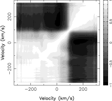
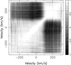
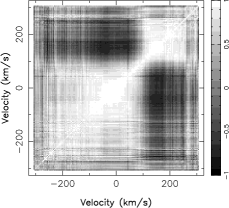
Figure 7: Mean H$\alpha$ (left), H$\beta$ (middle) and H$\gamma$ (right) profiles (top panel, full line) and associated standard deviations (top panel, dashed line), with corresponding autocorrelation matrices (bottom panel). Note that the standard deviation profiles are multiplied by 3 and shifted upwards by 1 for display purposes. In the lower panels, white indicates perfect correlation and black means perfect anticorrelation.

4.2 Balmer lines

H$\alpha$ and H$\beta$ lines exhibit strong emission with average equivalent widths of 900 and 200 km s^-1, (i.e., 2 and 0.32 nm) respectively. They exhibit clear rotational modulation and convey information that Ca ii IRT and He i emission lines do not contain (see Fig. 6). One obvious difference is that their unpolarised emission profiles are significantly broader (with full widths at half maximum of 190 and 90 km s^-1 for H$\alpha$ and H$\beta$ respectively) than their Zeeman signatures (70 km s^-1 wide). They also include a high-velocity component in their red wings (between $+100$ and $+300$ km s^-1) that alternately appears in absorption and emission (at cycles 0.75 and 1.21 respectively) but does not show up in the Stokes $V$ profile. Both points are readily visible on the average emission and standard deviation profiles of Balmer lines (see top panel of Fig. 7 for H$\alpha$ to H$\gamma$).

Autocorrelation matrices of Balmer emission profiles (see bottom panel of Fig. 7) reveal that the high-velocity redshifted component is anticorrelated with the central emission peak. We propose that the central Balmer emission peak, which varies in phase with the Ca ii and He i emission, is partly produced in the accretion shock. From its significant blueshift (7 km s^-1 with respect to the stellar velocity rest frame for H$\alpha$ and H$\beta$), the Balmer emission likely includes a wind component as well, strongest in H$\alpha$. The anti-correlated modulation of the high-velocity redshifted component points to a different origin; we suggest it is due to free-falling material in the preshock region of the accretion funnels.

5 Active regions and accretion spots

From the overview of the collected emission-line data in Sec. 4, we infer that rotational modulation is responsible for most of the observed variability in the Ca ii IRT and He i emission lines. We demonstrate in the present and following sections that this is also the case for the Stokes $I$ and $V$ LSD profiles of photospheric lines. As a first step, we use Doppler tomography to reconstruct the locations of dark spots on the surface of V2129 Oph from the time series of unpolarised photospheric line profiles. We also apply this Doppler imaging technique to the emission-line profiles, using them as accretion proxies to determine where the accretion spots are located.

Figure 8: Observed LSD Stokes $I$ (left panel) and Ca ii IRT emission core (right panel) of V2129 Oph (thin line) along with the maximum entropy fit to the data (thick line). The rotational phase and cycle of each observation is written next to each profile.

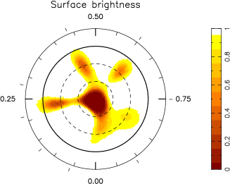
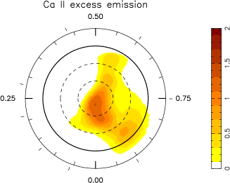
Figure 9: Surface maps of the local surface brightness relative to that of the quiet photosphere (left panel) and the local Ca ii excess emission relative to the basal chromospheric emission (right panel) on V2129 Oph, reconstructed from our series of ESPaDOnS LSD Stokes $I$ and Ca ii IRT emission line profiles (Fig. 8). The star is shown in flattened polar projection down to latitudes of $-30\hbox{${}^{\circ}$}$, with the equator depicted as a bold circle and parallels as dashed circles. Radial ticks around each plot indicate the phases of observation.

5.1 Dark spots

As we noted in Sec. 4, the distortions seen in the Stokes $I$ LSD profiles of V2129 Oph resemble those caused by cool photospheric features on the surfaces of active stars. Schevchenko & Herbst (1998) reach a similar conclusion from multicolour photometry. In the following, we model the observed LSD profile variations using tomographic imaging, assuming that dark surface features are present at the surface of V2129 Oph. We thus demonstrate that the temporal variations in the LSD profiles are mainly attributable to rotational modulation, and determine where dark spots are located on the surface of V2129 Oph.

We remove the veiling by simply scaling all profiles to the same equivalent width, and use the maximum entropy image reconstruction code of Brown et al. (1991) and Donati & Brown (1997) to adjust the surface image iteratively in order to optimise the fit to the series of Stokes $I$ profiles. The image quantity we reconstruct is the local surface brightness (relative to the quiet photosphere), varying from 1 (no spot) to 0 (no light). The local profile, assumed to be constant over the whole star, is obtained by matching a Unno-Rachkovski profile (Landi Degl’Innocenti, 2004) with no magnetic fields to the LSD profile of a K5 template star (61 Cyg) computed with the same line list as that used for V2129 Oph. The synthetic profiles we finally obtain (see Fig. 8, left panel) fit the observed Stokes $I$ LSD profiles at a level of about 0.15% or S/N=700 and confirms that the profile distortions are attributable to cool spots at the surface of the star.

Given the relative sparseness of our data set, one may argue that the success at fitting the Stokes $I$ LSD profiles is no more than a coincidence and does not truly demonstrate that the profiles are rotationally modulated. To check this, we varied the assumed rotation period of the star over a small interval about the value of Schevchenko & Herbst (1998) and reconstructed brightness images for each of the assumed rotation periods. We anticipate that the reconstructed image will show minimal spot coverage at the correct rotation period when the data are fitted at a fixed $\chi^{2}$, (or equivalently will yield the best fit to the data for a given spot coverage), if the profile variability is truly due to rotational modulation. This technique has also been used to derive constraints on the amount of differential rotation shearing the photosphere of V2129 Oph (Donati et al., 2000; Petit et al., 2002; Donati et al., 2003). Assuming solid body rotation, the optimal period we find is $6.56\pm 0.02$ d, compatible with the value of 6.53 d derived by Schevchenko & Herbst (1998). Assume now that the surface of the star rotates differentially, with the rotation rate varying with latitude $\theta$ as $\hbox{$\Omega_{\rm eq}$}-\hbox{$d\Omega$}\sin^{2}\theta$, $\Omega_{\rm eq}$ being the angular rotation rate at the equator and $d\Omega$ the difference in angular rotation rate between the equator and pole. We then find that optimal fits to the Stokes $I$ data are achieved for $\hbox{$\Omega_{\rm eq}$}=0.964\pm 0.003$ rad d^-1 and $\hbox{$d\Omega$}=0.054\pm 0.019$ rad d^-1, corresponding to rotation periods of 6.52 and 6.90 d for the equator and pole respectively. The error bar on $d\Omega$ is too large to detect unambiguously differential rotation at the surface of the star; we can however exclude values of $d\Omega$ that are either smaller than 0 or larger than 0.1 rad d^-1 (i.e., about twice the shear at the surface of the Sun). As a by-product, we very clearly demonstrate that the temporal variability of Stokes $I$ LSD profiles is due to rotational modulation.

The resulting map (see Fig. 9, left panel) includes one cool spot close to the visible pole and several additional ones at low to intermediate latitudes. The main polar spot is undoubtedly real. The low-latitude appendages at phases 0.23 and 0.95 are also well constrained by observed profiles featuring obvious line asymmetries. The two features centred on phase 0.44 and 0.62 are only associated with low level line asymmetries and their reality is less well established. The total area covered by photospheric cool spots in the reconstructed image is about 7%, with about 5% for the main polar spot only. We emphasize that this total spot coverage should be regarded as a lower limit. Doppler imaging recovers successfully the most significant brightness features, such as the cool polar spot seen here. Even if the stellar surface is peppered with spots much smaller than our resolution limit (e.g., Jeffers et al., 2006), such features will be suppressed, especially in stars with moderate rotation velocities.

We find that $\hbox{$v\sin i$}=14.5\pm 0.3$ km s^-1 and $\hbox{$v_{\rm rad}$}=-7.0\pm 0.2$ km s^-1  at the time of our observations, in perfect agreement with the recent published estimates ($15.2\pm 0.9$ and $-7.17\pm 0.25$ km s^-1, Eisner et al. 2005). Given the spectral resolution of ESPaDOnS (of about 5 km s^-1), the longitudinal resolution of the imaging process at the stellar equator is about 20^∘ or 0.05 rotation cycle. This is consistent with the longitudinal extent of the brightness features we recovered. We find that the information content of the brightness image is minimised for an axial inclination angle $i=45$^∘, in agreement with expectations from spectrophotometric estimates (see Sec. 2).

5.2 Accretion spots

We proceed in a similar way to model the fluctuations of the Ca ii IRT emission profiles and to retrieve information about the location of accretion spots at the surface of V2129 Oph. Thanks to their much smaller noise level, narrower width and simpler Zeeman signatures, and despite their weaker amount of rotational modulation, the Ca ii emission lines are a better choice than the He i line for this modelling task. The modelling accuracy is, however, limited by the intrinsic variability of the unpolarised emission lines. For this modelling, we use the simple two-component model described in Sec. 4, involving a basal chromospheric emission component evenly distributed over the surface of V2129 Oph and an accretion emission component arising in local accretion spots.

We now reconstruct an image of the local Ca ii excess emission from accretion spots relative to the basal chromospheric emission. We assume that the Ca ii minimum emission profile (at phase 0.28, see Fig. 3) provides a rough estimate of the basal chromospheric component. To model this chromospheric component, we use a Gaussian local profile with a full width at half maximum of 12 km s^-1 and an equivalent width of 15 km s^-1; given the $v\sin i$ estimate derived from Stokes $I$ LSD profiles, this model provides a reasonable match to the minimum emission profile at phase 0.28. We use the same local profile to model the accretion component. The fit we obtain is shown in Fig. 8 (right panel) while the reconstructed map is presented in Fig. 9 (right panel). As a result of intrinsic variability, the quality of the fit is poorer than that for photospheric lines. Using the last 6 profiles only improves the fit slightly but induces minimal changes in the resulting map. We conclude that the recovered image is robust despite the low-level intrinsic variability.

The map of Ca ii excess emission at the surface of V2129 Oph shares similarities with the distribution of dark spots. It shows in particular one main feature close to the pole and extending towards lower latitudes between phase 0.80 and 0.95, directly reflecting (i) the increased Ca ii emission at these phases and (ii) the fairly weak velocity change of the line emission core. Excess emission from this polar accretion spot reaches about 1.5 times that of the average quiet chromosphere; its relative area is about 5% of the total stellar surface. Given the finite resolution of the imaging process, the estimate we derive for the fractional area covered by accretion spots is likely an upper limit only.

6 The large-scale magnetic topology

In this section, we use stellar surface imaging to model the Zeeman signatures from both LSD profiles and accretion proxies. As in Sec. 5, our aim is to demonstrate that the variability of Stokes $V$ signatures is due to rotational modulation and to obtain a consistent description of the large-scale field topology of V2129 Oph.

6.1 Model description

The obvious difference between the sets of Zeeman signatures from the photospheric LSD profiles and the accretion proxies (see Sec. 4) led us to suggest that photospheric and emission lines do not form over the same regions of the stellar surface. This is compatible with our findings of Sec. 5 that the accretion emission is concentrated in the dark polar regions. The low surface brightness is expected to suppress the photospheric Zeeman signature, rendering the photospheric lines insensitive to the field. In the following, we assume this to be the case and demonstrate that both sets of Zeeman signatures are nonetheless consistent with a single large-scale magnetic topology.

As in Sec. 5, we use the Ca ii IRT lines as our preferred accretion proxy. We describe it with the two-component model of Sec. 4, combining a basal chromospheric emission component evenly distributed over the star with an additional emission component concentrated in local accretion spots. The emission-line Zeeman signatures are assumed to be associated with the accretion component only, as supported by the conclusions of Sec. 4.

The model we adopt involves a vector magnetic field $B$ and a local accretion filling-factor $f$ which describes the local sensitivity to accretion proxies and photospheric lines. For $f=0$, the local area on the protostar’s surface contributes fully to photospheric lines and generates no Ca ii excess emission (and only unpolarised chromospheric Ca ii emission); for $f=1$, the local area does not contribute at all to photospheric lines and produces the maximum amount of excess Ca ii emission and polarisation (in addition to the unpolarised chromospheric Ca ii emission). Spectral contributions for intermediate values of $f$ are derived through linear combinations between the $f=0$ and $f=1$ cases. We obtain both $B$ and $f$ by fitting the corresponding synthetic Stokes $V$ profiles to the observed Zeeman signatures from both LSD profiles and Ca ii emission cores. We can also incorporate the additional constraint of fitting the unpolarised profiles of the Ca ii emission cores.

The code we use for fitting $B$ and $f$ is adapted from the stellar surface magnetic imaging code of Donati et al. (2001) and Donati et al. (2006). In this model, the surface of the star is divided into a grid of thousands of small surface pixels, on which we reconstruct $B$ as a 3 component vector field and $f$ as a simple scalar field. The magnetic vector field is described and computed as a spherical-harmonic expansion, whose coefficients are determined through fitting the simulated Stokes $V$ profiles to the observed data sets. More specifically, the field is expressed as the sum of a poloidal field and a toroidal field, with the three field components in spherical coordinates being defined through three sets of complex spherical harmonics coefficients, $\alpha_{\ell,m}$, $\beta_{\ell,m}$ and $\gamma_{\ell,m}$. Here $\ell$ and $m$ denote the order and degree of the spherical-harmonic mode.

For a given magnetic topology, the unpolarised and polarised spectral contributions to photospheric lines are obtained through the Unno-Rachkovsky model used in Sec. 5, and assuming a Landé factor and mean wavelength of 1.2 and 620 nm respectively. For the excess Ca ii emission produced in the accretion region, we assume the same Gaussian model as that of Sec. 5, with an equivalent width set to twice that of the quiet chromosphere profile (thus defining the highest possible amount of local excess emission), a unit Landé factor and a mean wavelength of 850 nm.

Figure 10: Stokes $V$ Zeeman signatures (thin line) from LSD profiles of photospheric lines (left column) and Ca ii emission cores (right column) along with the maximum entropy fit to the data (thick line). The rotational phase and cycle of each observation is written next to each profile. A 3$\sigma$ error bar is also shown to the left of each profile.

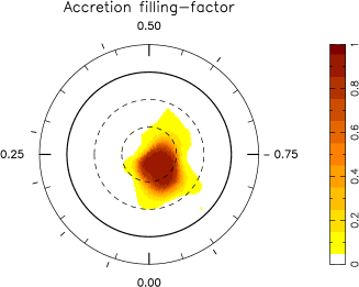
Figure 11: Map of the local accretion filling factors at the surface of V2129 Oph, as derived from simultaneously fitting the two series of Zeeman signatures (LSD profiles of photospheric lines and Ca ii emission cores, see Sec. 4) and assuming that each series senses a different spatial region of the stellar surface (see Sec. 6).

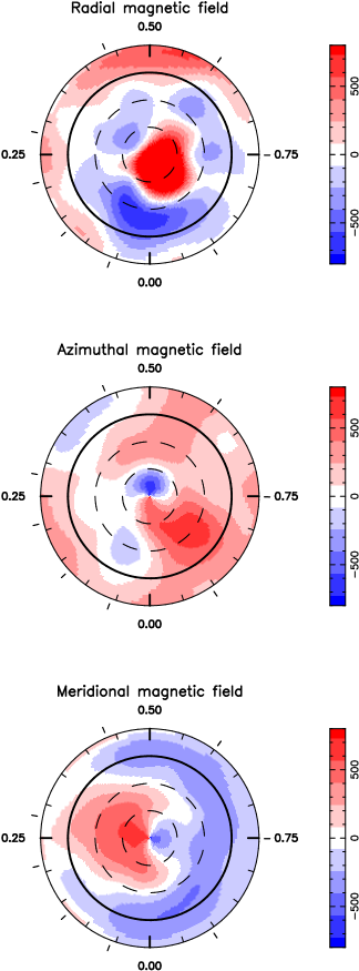
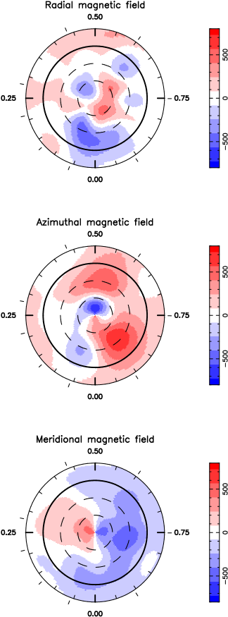
Figure 12: Reconstructed magnetic topology of V2129 Oph, simultaneously derived from our two series of Zeeman signatures (LSD profiles of photospheric lines and Ca ii  emission cores, see Sec. 4, left panel) and when using LSD Stokes $V$ profiles from photospheric lines only (right panel). The image on the right misses most of the 2 kG high-latitude region of positive radial field, in which accretion occurs. The three components of the field in spherical coordinates are displayed (from top to bottom) in both cases, with field fluxes labelled in G.

  

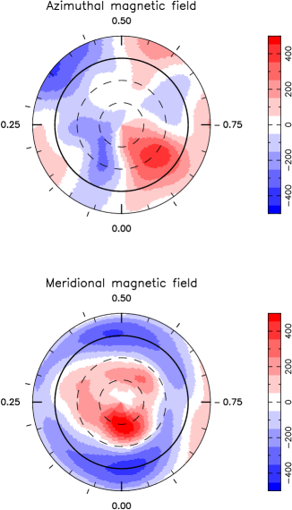
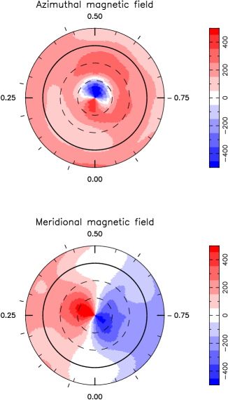
Figure 13: Decomposition of the azimuthal and meridional components of the reconstructed field (see Fig. 12, left column) into their non-radial poloidal (left column) and toroidal (right column) terms, corresponding respectively to spherical-harmonic coefficients $\beta_{\ell,m}$ and $\gamma_{\ell,m}$.

Given the spatial resolution of the imaging process (see Sec. 5), we find it sufficient to limit the spherical-harmonic expansion of the magnetic field components to terms with $\ell\leq 20$ (230 modes altogether). In practice, little improvement is obtained when adding spherical harmonic terms corresponding to $\ell\geq 15$.

6.2 Modelling results

We find that the Stokes $V$ signatures of both the photospheric LSD profiles and the Ca ii emission cores can be fitted simultaneously down to the noise level using the model described in Sec. 10 above. Repeating the experiment for a range of rotation periods (as we did in Sec. 5 for Stokes $I$ profiles only) and assuming solid body rotation yields optimal fits to the Stokes $V$ data at a period of $6.62\pm 0.07$ d, again consistent with the 6.53 d period derived by Schevchenko & Herbst (1998). Assuming now that the star rotates differentially, we find that optimal fits to the Stokes $V$ profiles are achieved for $\hbox{$\Omega_{\rm eq}$}=0.928\pm 0.020$ rad d^-1 and $\hbox{$d\Omega$}=-0.038\pm 0.030$ rad d^-1, compatible within 3$\sigma$ with the values derived from the Stokes $I$ profiles. This confirms our earlier conclusion from inspection of the profiles in Sec. 4 that rotational modulation dominates the temporal variability of the Zeeman signatures.

The maps of local accretion filling-factors and magnetic field derived from the Stokes $V$ data are shown in Figs. 11 and 12 (left panel). They confirm and strengthen the conclusion that accretion is very localised at the stellar surface, being concentrated in a high-latitude region where the radial field reaches a peak value of 2.1 kG, in agreement with the estimate derived in Sec. 4. This accretion region occupies about 5 percent of the total stellar surface. Including a simultaneous fit to the unpolarised Ca ii  emission profiles has little effect on the result, provided we assume the local Ca ii excess emission in the accretion regions to be about twice the emission from the quiet chromosphere. Note that this fractional area is only an upper limit. A similar fit to the data can be obtained by assuming that the local Ca ii  excess emission in the accretion spot is larger than that considered here. In this case, we obtain a smaller accretion hot spot whose average location is unchanged. The spatial resolution is however high enough to claim that the accretion spot cannot be larger than the one we reconstruct.

As a comparison, we also show in Fig. 12 (right panel) the magnetic field topology reconstructed from using the photospheric Stokes $V$ LSD profiles alone. Unsurprisingly, this topology is essentially the same as that in the left-hand panel for all regions where no accretion occurs and for which all available information comes from the photospheric lines. This map, however, misses most of the magnetic flux from the high-latitude accretion spot, which now shows up as a weak positive field feature only.

     

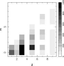
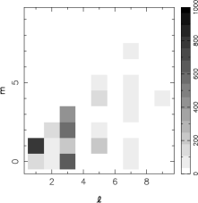
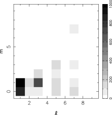
Figure 14: Modulus (in G) of the spherical-harmonic complex coefficients $\alpha_{\ell,m}$, $\beta_{\ell,m}$ and $\gamma_{\ell,m}$ (from left to right, see text) for the reconstructed field topology of V2129 Oph (Fig. 12, left column), as a function of mode degree $\ell$ and order $m$. In this case, the imaging code was pushed towards antisymmetric field configurations by favouring modes with odd $\ell$ values. Modes with $\ell<10$ only are displayed here.

6.3 Field topology

Even though it is dominated by a 2 kG high-latitude positive radial field feature, the magnetic topology nevertheless differs significantly from a dipole and exhibits a number of clear specific features. In particular, we find that the fit to the data (and in particular to the Stokes $V$ LSD profiles) is significantly poorer if we assume that the field is purely poloidal, implying that the toroidal field component we reconstruct is likely to be real. The spatial structure of this toroidal component is shown on Fig. 13 (right column) along with the non-radial poloidal field component (left column).

The large-scale field topology includes a strong axisymmetric component. The poloidal field component features a strong positive radial field spot near the pole, surrounded by a negative radial field ring located slightly above the equator (see top left image of Fig. 12), suggesting a dominant axisymmetric mode with $\ell$ higher than 1. This is also visible from the dual ring structure in the meridional component of the poloidal field (see bottom left image of Fig. 13). The toroidal field topology is simple (see right panel of Fig. 13) and comprises a ring of counter-clockwise oriented field. This unipolar ring is tilted with respect to the rotation axis towards phase 0.55 and passes through the rotation pole, giving it a complex multipolar appearance when plotted in spherical coordinates.

Since the lower hemisphere of V2129 Oph is poorly constrained by observations (southern surface features being strongly limb-darkened and only visible for a short fraction of the rotation cycle), there is no direct way of working out whether the large-scale field topology is mainly symmetric or antisymmetric with respect to the centre of the star, or whether it features a mixed combination of symmetric and antisymmetric modes. By forcing the code towards either symmetric or antisymmetric topologies or by letting it choose by itself, we find that all three options are possible and correspond to magnetic topologies that are very similar over the visible hemisphere and that fit the observations equally well. While the mainly symmetric and antisymmetric magnetic topologies we reconstruct both include a strong field region near the invisible pole (mirroring that detected close to the visible pole, with equal and opposite polarities respectively), the third solution mixes both symmetric and antisymmetric solutions in roughly equal proportions and produces a topology with no strong field region in the invisible hemisphere. Assuming that magnetic topologies of cTTSs are either mainly symmetric or antisymmetric (most of them featuring strong unipolar field regions close to the pole, Valenti & Johns-Krull 2004; Symington et al. 2005a), we find that the mainly antisymmetric field topology is more likely as it requires a field with lower contrast for the same quality of the fit to the data.

In this antisymmetric case, the dominant mode of the reconstructed large-scale field corresponds to an octupole ($\ell=3$), with only little energy reconstructed in the dipole field configuration. Fig. 14 shows how the reconstructed magnetic energy is distributed among the various modes. While the toroidal field term is mainly confined to low order modes (mostly $\ell=1$), the poloidal field extends to modes with at least $\ell=5$ – with a maximum at $\ell=3$ – and tends to concentrate mostly in axisymmetric modes with small $m$ values. Note that, given the limited resolution of our imaging process, we miss all magnetic flux at small spatial scales (e.g. in the form of closed bipolar groups) that may be present on V2129 Oph.

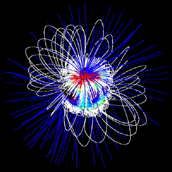
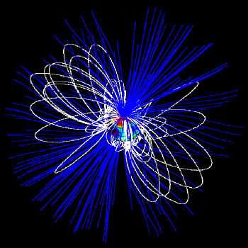
Figure 15: Magnetospheric topology of V2129 Oph as derived from potential extrapolations of the reconstructed surface magnetic topology (left panel of Fig. 12). The magnetosphere is assumed to extend up to the inner disc radius, equal to 3.4 and 6.8 $R_{\star}$ in the left and right panels respectively. The complex magnetic topology close to the surface of the star is very obvious. In both cases, the star is shown at rotational phase 0.8. The colour patches at the surface of the star represent the radial component of the field (with red and blue corresponding to positive and negative polarities); open and closed field lines are shown in blue and white respectively.

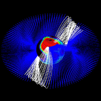
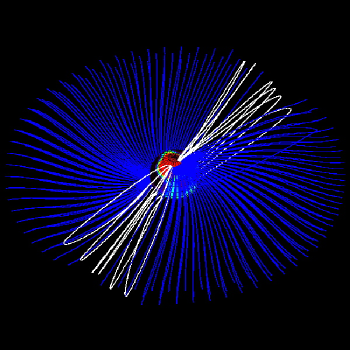
Figure 16: Locations of field lines capable of accreting material from the accretion disc to the surface of V2129 Oph, as derived from the magnetospheric topologies shown in Fig. 15. Open field lines connecting to the disc are shown in blue, while closed field lines appear in white. As in Fig. 15, the magnetosphere is assumed to extend to either 3.4 or 6.8 $R_{\star}$ (left and right panels respectively). The topology of the accretion columns becomes much more complex when the magnetosphere is assumed to be smaller.

7 Magnetospheric accretion and corona

To illustrate how accretion proceeds between the inner disc and the surface of the star, we extrapolate the reconstructed magnetic field over the whole magnetosphere. To do this, we assume that the 3D field topology is mainly potential and becomes radial beyond a certain magnetospheric radius $r_{\rm A}$ from the star, to mimic the opening of the largest magnetic loops under the coronal pressure (Jardine et al., 2002, 2006; Gregory et al., 2006). In non-accreting stars, this distance is usually assumed to be smaller than or equal to the corotation radius ($r_{\rm C}$) at which the Keplerian orbital period equals the stellar rotation period. In cTTSs however, the magnetic field of the protostar is presumably clearing out the central part of the accretion disc, suggesting that the magnetosphere should extend as far as the inner disc rim (Jardine et al., 2006). The derived magnetospheric maps (see Fig. 15 for two possible values of $r_{\rm A}$) clearly show that the field topology is complex, with an intricate network of closed loops at the surface of the star. As $r_{\rm A}$ is increased, the magnetosphere is dominated by more extended open and closed field lines.

For several reasons, our description of the magnetosphere is only an approximation. The innermost field geometry is likely to be more complex than our reconstruction, as small-scale magnetic structures at the surface of the star remain undetected through spectropolarimetry. This is not, however, a crucial issue for the present study, which focusses mainly on the medium- and large-scale magnetic topology of V2129 Oph. Moreover, the true magnetic topology of V2129 Oph is likely not potential given the strong plasma flows linking the disc to the stellar surface and the significant toroidal field component detected at the surface of V2129 Oph. Finally, the magnetic field in the disc is also expected to interact with the magnetosphere, at least in its outer regions (e.g., von Rekowski & Brandenburg, 2004). These complications are not, however, included in most existing theoretical studies on magnetospheric accretion (e.g., Romanova et al., 2003, 2004). We thus believe that, despite its limitations, our imaging study should be robust enough to yield the rough locations of accretion funnels and to provide a useful illustration of the constraints that spectropolarimetric data sets can yield. More quantitative analysis and simulations are postponed to forthcoming papers.

We can estimate where the accretion funnels are located and where they are anchored at the surface of the star, by identifying those magnetospheric field lines that are able to accrete material from the disc. Such field lines must link the star to the disc and intersect the rotational equator with effective gravity pointing inwards in the co-rotating frame of reference (e.g. Gregory et al., 2006; Gregory et al., 2007).

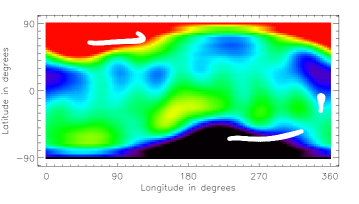
Figure 17: Location of the footpoints of accreting field lines at the surface of the star (white circles), assuming that the magnetosphere extends to 6.8 $R_{\star}$. In this case, accreting field lines concentrate almost exclusively in the strong unipolar radial field regions at high latitudes. The colours at the surface of the star depict the radial field component (with red and blue corresponding to positive and negative polarities). Note that phase runs backwards with longitude, i.e., decreases from 1 to 0 while longitude increases from 0^∘ to 360^∘.

If we assume that $\hbox{$r_{\rm A}$}=3.4$ $R_{\star}$, we find that disc material accretes mainly on to the radial field spots located close to the equator, with only a small fraction of the accretion flow reaching the high-latitude spots. This is obviously in strong contradiction with the conclusions of Sec. 6. If we assume a more extended magnetosphere with $\hbox{$r_{\rm A}$}=6.8$ $R_{\star}$, most of the accreting material flows onto the high-latitude accretion spots. Pushing $r_{\rm A}$ further out (to 7.5 $R_{\star}$) focusses all the accreting material at high latitudes only, in much better agreement with observations (see Figs 16 and 17). We therefore conclude that $r_{\rm A}$ is closer to 7 $R_{\star}$ in V2129 Oph and likely coincides with $r_{\rm C}$, equal to $0.075\pm 0.003$ AU or $6.8\pm 1.2$ $R_{\star}$.

In the magnetospheric topology we derive, the northern accretion funnel passes in front of the high-latitude accretion hot spot between rotation phases 0.7 and 0.8. We suggest that free-falling material in this accretion funnel is responsible for the high-velocity absorption component observed in the red wing of Balmer lines at cycle 0.75 (see Sec. 4), just as solar prominences transiting the solar disc are viewed as dark filaments. Similarly, we propose that free-falling plasma along the southern accretion funnel that plunges into the invisible accretion spot produces, through scattering, the redshifted emission component that Balmer lines feature at cycle 1.21. The orientation of the southern accretion funnel is indeed ideally oriented for this purpose at this particular rotation phase. Detailed radiative transfer computations (e.g., Symington et al., 2005b; Kurosawa et al., 2006) are needed to confirm this.

The magnetospheric field geometry derived from the reconstructed field maps can also be used to model the corona of V2129 Oph and estimate the associated X-ray flux. Assuming $\hbox{$r_{\rm A}$}=7$ $R_{\star}$ and an isothermal corona at a temperature of 20 MK (typical for the hot component of X-ray emission from cTTSs) filled with plasma in hydrostatic equilibrium (e.g. Jardine et al., 2006; Gregory et al., 2006), we obtain an X-ray emission measure of $4\times 10^{53}$ cm^-3 and an average (i.e., emission-measure-weighted) coronal density of $5\times 10^{9}$ cm^-3. This value is typical for solar-mass cTTSs such as V2129 Oph according to the statistics derived from the COUP (Chandra Orion Ultradeep Project) survey (e.g., Jardine et al., 2006). It translates into a X-ray luminosity of $4\times 10^{30}$ erg s^-1, matching well the published value of $2.5\times 10^{30}$ erg s^-1 (Casanova et al., 1995).

8 Discussion

The spectropolarimetric data we have collected on V2129 Oph yields the first realistic model of the large-scale magnetic topology on a mildly accreting cTTS. Although this first study of its kind addresses only one star, V2129 Oph can nevertheless be regarded as prototypical of mildly accreting cTTSs, exhibiting no behaviour that would mark this star out as peculiar. We can thus use it to readdress a number of issues regarding cTTSs.

8.1 Cool spots and hot accretion regions

We observe that profile variations due to intrinsic variability (e.g., resulting from unsteady accretion flows) are smaller than those caused by rotational modulation, for both the photospheric lines and the accretion proxies. This conclusion is already robust and confirms previous published results based on data sets with similar time sampling and coverage to ours (e.g., Valenti & Johns-Krull, 2004). Future observations spanning timescales of at least 2 complete rotation cycles, would be welcome to establish whether this situation is typical.

The photospheric line profiles of V2129 Oph are variable in shape and to a lesser extent in strength. The profile distortions consist of bumps (rather than dips) and can be attributed to the presence of cool spots at the surface of the star, rotating in and out of the observer’s view. This confirms the conclusions of Schevchenko & Herbst (1998), who deduced from the photometric colour variations that the brightness inhomogeneities on V2129 Oph are mostly due to cool and dark spots rather than to bright and hot regions. With Doppler imaging, we successfully reproduce the rotational modulation of photospheric line shapes and find that the surface spot distribution is dominated by a cool region over the visible pole. In this respect, this spot distribution differs from those of cool active stars with similar characteristics, which usually do not show polar features at rotation periods longer than about one week (e.g., the K1 evolved RS CVn subgiant II Peg, Petit et al. 2006).

Accretion spots are also present at the surface of the star. Their spectral signatures are not seen at photospheric level, but show up clearly in emission proxies such as the Ca ii IRT and He i lines which usually trace heating of the star’s upper atmospheric layers.

These emission proxies include two components: a stationary emission component presumed to originate in a quiet chromosphere covering the whole stellar surface, and a rotationally-modulated emission feature presumably formed in local accretion spots. The accretion component exhibits only small-amplitude radial velocity modulation, indicating that accretion spots are located at high latitudes. This is confirmed through tomographic imaging, which shows that accretion on the visible hemisphere of V2129 Oph is concentrated in a single high-latitude spot covering less than 5% of the stellar surface, located within the main cool polar spot detected at photospheric level. It suggests that the heat produced in the accretion shock is not transferred to the photosphere efficiently enough to warm it up above the temperature of the non-accreting photosphere. We speculate that a second accretion spot is present near the invisible pole, at a location symmetrical with respect to the centre of the star.

We also find that differential rotation of V2129 Oph is comparable with or less than that of the Sun, in agreement with previous observations (Johns-Krull, 1996) and theoretical predictions (Küker & Rüdiger, 1997). Our result invalidates in particular early suggestions that cTTSs might be strong differential rotators (Smith, 1994).

8.2 Magnetic topology and origin of the field

We observe that rotational modulation dominates the temporal evolution of the Stokes $V$ profiles of both photospheric lines and accretion proxies. Comparing Zeeman signatures from both data sets suggests that they form in different complementary regions of the stellar surface, with accretion proxies tracing magnetic fields at the footpoints of accretion funnels and photospheric lines diagnosing fields in the non-accreting photosphere. With this assumption, we are able to reconstruct, through tomographic imaging, a consistent magnetic topology that simultaneously reproduces both sets of Zeeman signatures.

Despite being anchored in 2 kG high-latitude radial field spots, the reconstructed magnetic field is more complex than the simple dipole assumed in most theoretical models of magnetospheric accretion (e.g., Romanova et al., 2003, 2004). The negative radial field ring encircling the main positive radial field pole provides direct evidence that the large-scale poloidal field structure corresponds to spherical harmonics order $\ell\geq 2$. We find that the field of V2129 Oph is more likely to be mainly antisymmetric (rather than symmetric) with respect to the centre of the star; the respective contributions to the 2 kG radial field region from the $\ell=1$ (tilted dipole), $\ell=3$ (tilted octupole) and $\ell=5$ terms are about 0.35, 1.2 and 0.6 kG. The reconstructed field also includes a toroidal field component in the form of a tilted ring of counterclockwise azimuthal field.

Given that fossil magnetic fields are presumably dissipated very quickly in largely convective stars (e.g., Chabrier & Küker, 2006), the most natural assumption is that large-scale fields of cTTSs are generated through dynamo action. The mainly axisymmetric field reconstructed on V2129 Oph argues in this direction. The magnetic topology seen here, however, differs in important respects from those of moderately rotating cool active stars with similar characteristics (e.g., Petit et al., 2006). The strong high-latitude unipolar field region detected on V2129 Oph and the relatively strong $\ell\geq 3$ orders of the large-scale field are the most obvious. These differences suggest that cTTSs may feature a composite field, including both fossil and dynamo components. More data are needed to confirm this and to explore the potential impact on stellar formation.

8.3 Disc-star magnetic coupling

Several theoretical papers (e.g., Königl, 1991; Shu et al., 1994; Cameron & Campbell, 1993) studied how the stellar magnetic field interacts with the surrounding accretion disc and disrupts its vertical structure close to the star. They showed further that the balance between accretion torques and angular momentum losses causes the rotation of the star to evolve towards an equilibrium in which the disc disruption radius lies close to $r_{\rm A}$ and just inside the co-rotation radius $r_{\rm C}$. Assuming different models of the star/disc interaction, these authors derived convenient expressions for $r_{\rm A}$; they proposed that this coupling causes cTTSs to slow down to the Keplerian orbital period at $r_{\rm A}$ (thus equating $r_{\rm A}$ and $r_{\rm C}$), explaining why cTTSs are on average rotating more slowly than their disc-less equivalents. This scenario is refered to as ’disc-locking’ in the literature.

These papers can be used to estimate $r_{\rm A}$ as a function of the mass, radius, mass-accretion rate and magnetic dipole strength of the protostar. Using values listed in Sec. 2 and a dipole strength of 0.35 kG (see Sec. 6), we find that $r_{\rm A}$ can be as low as 2 $R_{\star}$ if using the model of Königl (1991) or Shu et al. (1994), i.e., far smaller than $r_{\rm C}$ (about 7 $R_{\star}$). The model of Cameron & Campbell (1993), yielding $r_{\rm A}$ values of 5.1 to 8.1 $R_{\star}$ (in better agreement with $r_{\rm C}$), appears to provide a better quantitative description of the star/disc magnetic interaction assuming this coupling is responsible for the slow rotation of V2129 Oph.

The disc-locking scenario was recently criticised on various grounds. Observations revealed that surface magnetic strengths on cTTSs (measured from Zeeman magnetic broadening of unpolarised profiles) do not correlate well with those expected from theoretical models, casting doubts on the validity of the disc-locking mechanism (e.g., Bouvier et al., 2007; Johns-Krull, 2007). On theoretical grounds, authors claimed that a wind from the protostar would blow the field open at 3 $R_{\star}$ (e.g., Safier, 1998; Matt & Pudritz, 2004) and prevent magnetic coupling between the star and disc.

Our study however demonstrates that the most relevant physical quantity for studying this issue is not the surface magnetic field itself, but rather the large-scale dipole strength on which magnetic coupling mostly depends. On V2129 Oph at least, the large-scale dipole component is compatible with the predictions of Cameron & Campbell (1993). Moreover, our observations establish that accretion occurs onto the polar regions of V2129 Oph rather than the equator, a phenomenon which we can only explain if the high-latitude field links to the accretion disc at a distance of about 7 $R_{\star}$. This is obviously not compatible with the field being blown open by the wind at 3 $R_{\star}$.

9 Conclusion

In this paper, we report the discovery of magnetic fields on the cTTS V2129 Oph using ESPaDOnS, the new stellar high-resolution spectropolarimeter recently installed at CFHT. Circular polarisation Zeeman signatures are detected in photospheric lines and in emission lines tracing magnetospheric accretion. We demonstrate that the temporal variations of both unpolarised and circularly polarised profiles, monitored over the complete rotational cycle of V2129 Oph, are mostly attributable to rotational modulation.

From our sets of Zeeman signatures from photospheric lines and accretion proxies simultaneously, we recover the medium- and large-scale magnetic topology at the surface of V2129 Oph using tomographic imaging tools. In this process, we also successfully derive the location of the accretion regions, tracing the footpoints of accretion funnels at the surface of the star. We find that the magnetic topology of V2129 Oph is significantly more complex than a dipole and is dominated by a 1.2 kG octupole, tilted by about 20^∘ with respect to the rotation axis. The large-scale dipole component is much smaller, with a polar strengh of only 0.35 kG. The magnetic field is mainly antisymmetric with respect to the centre of the star, and the accretion regions are found to coincide with the two main high-latitude magnetic poles (each covering about 5% of the total stellar surface). The high-latitude accretion spots apparently coincide with dark polar features at photospheric level. The magnetic topology of V2129 Oph is unusually complex compared to those of non-accreting cool active subgiants with moderate rotation periods.

As an illustration, we also provide a first attempt at modelling the magnetospheric topology and accretion funnels of V2129 Oph using field extrapolation. We find that the magnetosphere must extend to distances of about 7 $R_{\star}$ to produce accretion funnels that match the observations and anchor in the high-latitude accretion spots identified at the stellar surface. This distance is roughly equal to the corotation radius and matches the theoretical predictions of Cameron & Campbell (1993), suggesting that the star/disc magnetic coupling can possibly explain the slow rotation of V2129 Oph. It suggests that magnetic field lines from the protostar are apparently capable of coupling to the accretion disc beyond 3 $R_{\star}$. The accretion geometry we derive is qualitatively consistent with the modulation of Balmer lines and consistent with the X-ray coronal fluxes typical of cTTSs.

More similar data sets are required to check how the conclusions of this prototypical study apply to other cTTSs, with different masses, rotation and accretion rates.

References

- Bontemps et al. (2001) Bontemps S., André P., Kaas A., Nordh L., Olofsson G., Huldtgren M., Abergel A., Blommaert J., Burgdorf M., Cesarsky C., Cesarsky C., Copet E., Davies J., Falgarone E., Lagache G., Montmerle T., Pérault M., 2001, A&A, 372, 173
- Bouvier (1990) Bouvier J., 1990, AJ, 99, 946
- Bouvier et al. (2007) Bouvier J., Alencar S., Harries T., Johns-Krull C., Romanova M., 2007, in Reipurth B., Jewitt D., Keil K., eds, Protostars and Planets V Vol. 951. University of Arizona Press, p. 479
- Bouvier & Appenzeller (1992) Bouvier J., Appenzeller I., 1992, A&AS, 92, 481
- Brown et al. (1991) Brown S., Donati J.-F., Rees D., Semel M., 1991, A&A, 250, 463
- Cameron & Campbell (1993) Cameron A., Campbell C., 1993, A&A, 274, 309
- Casanova et al. (1995) Casanova S., Montmerle T., Feigelson E., André P., 1995, ApJ, 439, 752
- Chabrier & Küker (2006) Chabrier G., Küker M., 2006, A&A, 446, 1027
- Daou et al. (2006) Daou A., Johns-Krull C., Valenti J., 2006, ApJ, 635, 466
- Donati & Brown (1997) Donati J.-F., Brown S., 1997, A&A, 326, 1135
- Donati et al. (2003) Donati J.-F., Cameron A., Petit P., 2003, MNRAS, 345, 1187
- Donati et al. (2003) Donati J.-F., Cameron A., Semel M., Hussain G., Petit P., Carter B., Marsden S., Mengel M., Lopez Ariste A., Jeffers S., Rees D., 2003, MNRAS, 345, 1145
- Donati et al. (2006) Donati J.-F., Howarth I., Jardine M., Petit P., Catala C., Landstreet J., Bouret J.-C., Alecian E., Barnes J., Forveille T., Paletou F., Manset N., 2006, MNRAS, 370, 629
- Donati et al. (2000) Donati J.-F., Mengel M., Carter B., Marsden S., Cameron A., Wichmann R., 2000, MNRAS, 316, 699
- Donati et al. (1997) Donati J.-F., Semel M., Carter B., Rees D., Collier Cameron A., 1997, MNRAS, 291, 658
- Donati et al. (2001) Donati J.-F., Wade G., Babel J., Henrichs H., de Jong J., Harries T., 2001, MNRAS, 326, 1256
- Doppmann et al. (2003) Doppmann G., Jaffe D., White R., 2003, AJ, 126, 3043
- Eisner et al. (2005) Eisner J., Hillenbrandt L., White R., Akeson R., Sargent A., 2005, ApJ, 623, 952
- Geoffray & Monin (2001) Geoffray H., Monin J.-L., 2001, A&A, 369, 239
- Gregory et al. (2006) Gregory S., Jardine M., Simpson I., Donati J.-F., 2006, MNRAS, 371, 999
- Gregory et al. (2007) Gregory S., Jardine M., Wood K., 2007, MNRAS, in press (astro-ph/0704.2958)
- Jardine et al. (2006) Jardine M., Cameron A., Donati J.-F., Gregory S., Wood K., 2006, MNRAS, 367, 917
- Jardine et al. (2002) Jardine M., Wood K., Cameron A., Donati J.-F., Mackay D., 2002, MNRAS, 336, 1364
- Jeffers et al. (2006) Jeffers S., Barnes J., Cameron A., Donati J.-F., 2006, MNRAS, 366, 667
- Johns-Krull (1996) Johns-Krull C., 1996, A&A, 306, 803
- Johns-Krull (2007) Johns-Krull C., 2007, ApJ, in press (astro-ph/0704.2923)
- Johns-Krull et al. (1999) Johns-Krull C., Valenti J., Hatzes A., Kanaan A., 1999, ApJ, 510, L41
- Johns-Krull et al. (1999) Johns-Krull C., Valenti J., Koresko C., 1999, ApJ, 516, 900
- Königl (1991) Königl A., 1991, ApJ, 370, L39
- Küker & Rüdiger (1997) Küker M., Rüdiger G., 1997, A&A, 328, 253
- Kurosawa et al. (2006) Kurosawa R., Harries T., Symington N., 2006, MNRAS, 370, 580
- Kurucz (1993) Kurucz R., 1993, CDROM # 13 (ATLAS9 atmospheric models) and # 18 (ATLAS9 and SYNTHE routines, spectral line database). Smithsonian Astrophysical Observatory, Washington D.C.
- Landi Degl’Innocenti (2004) Landi Degl’Innocenti E., 2004, Polarisation in Spectral Lines. Vol. 307 of Astrophysics and Space Science Library, Kluwer Academic Publishers
- Matt & Pudritz (2004) Matt S., Pudritz R., 2004, ApJ, 607, L43
- Mohanty et al. (2005) Mohanty S., Jayawardhana R., Basri G., 2005, ApJ, 626, 498
- Padgett (1996) Padgett D., 1996, ApJ, 471, 847
- Petit et al. (2006) Petit P., Donati J.-F., Aurière M., Landstreet J., Lignières F., Marsden S., Mouillet D., Paletou F., Toqué N., Wade G., 2006, in Casini R., Lites B., eds, Solar Polarization Workshop #4 Vol. 358 of ASP Conf. Proc.
- Petit et al. (2002) Petit P., Donati J.-F., Cameron A., 2002, MNRAS, 334, 374
- Romanova et al. (2004) Romanova M., Utsyugova G., Koldoba A., Lovelace R., 2004, ApJ, 610, 920
- Romanova et al. (2003) Romanova M., Utsyugova G., Koldoba A., Wick J., Lovelace R., 2003, ApJ, 595, 1009
- Safier (1998) Safier P., 1998, ApJ, 494, 336
- Schevchenko & Herbst (1998) Schevchenko V., Herbst W., 1998, AJ, 116, 1419
- Shu et al. (1994) Shu F., Najita J., Ostriker E., Wilkin F., Ruden S., Lizano S., 1994, ApJ, 429, 781
- Siess et al. (2000) Siess L., Dufour E., Forestini M., 2000, A&A, 358, 593
- Smith (1994) Smith M., 1994, A&A, 287, 523
- Symington et al. (2005b) Symington N., Harries T., Kurosawa R., 2005b, MNRAS, 356, 1489
- Symington et al. (2005a) Symington N., Harries T., Kurosawa R., Naylor T., 2005a, MNRAS, 358, 977
- Valenti & Johns-Krull (2004) Valenti J., Johns-Krull C., 2004, Ap&SS, 292, 619
- von Rekowski & Brandenburg (2004) von Rekowski B., Brandenburg A., 2004, A&A, 420, 17
- Yang et al. (2005) Yang H., Johns-Krull C., Valenti J., 2005, ApJ, 635, 466