Abstract

This paper investigates the Arnowitt–Deser–Misner (hereafter ADM) form of spherically symmetric gravity with variable Newton parameter $G$ and cosmological term $\Lambda_{c}$. The Newton parameter is here treated as a dynamical variable, rather than being merely an external parameter as in previous work on closely related topics. The resulting Hamilton equations are obtained; interestingly, a static solution exists, that reduces to Schwarzschild geometry in the limit of constant $G$, describing a Newton parameter ruled by a nonlinear differential equation in the radial variable $r$. A remarkable limiting case is the one for which the Newton parameter obeys an almost linear growth law at large $r$. An exact solution for $G$ as a function of $r$ is also obtained in the case of vanishing cosmological constant. Some observational implications of these solutions are obtained and briefly discussed.

I Introduction

The last ten years have witnessed an encouraging progress in the application of renormalization-group methods to the nonperturbative renormalization of Quantum Einstein Gravity Reut98 ; Laus05 ; Nied06 ; Nied07 . In general, field theories which are nonperturbatively renormalizable are constructed by performing the limit of infinite ultraviolet cutoff at a nonGaussian renormalization group fixed point $g_{*i}$ in the space $\left\{g_{i}\right\}$ of all dimensionless couplings $g_{i}$ which parametrize a general action functional. In the case of general relativity, an effective average action has been built Reut98 , and such a nonGaussian ultraviolet fixed point has been found in the case of the Einstein–Hilbert and higher-derivative truncations Laus05 .

Several cosmological applications of this framework have also been considered. For example, in Weye06 (see also Weye04 ) it has been argued that the resulting scale dependence of the Newton parameter at large distances might mimic the presence of dark matter at galactic and cosmological scales. On the other hand, in early work by some of us Bona04 , we had tried to build an action functional where the running of the Newton parameter is ruled by suitable Euler–Lagrange or Hamilton equations, while being compatible with the renormalization-group flow in the neighbourhood of an ultraviolet fixed point. For this purpose, one adds to an action of the Einstein–Hilbert type (but with variable $G$, so that it is brought within the integrand) two compensating terms such that the action reduces to the York–Gibbons–Hawking York72 ; Gibb77 action for fixed $G$ and $\Lambda_{c}$, and takes the same functional form as in the ADM formalism for general relativity (see Eq. (2.1) below).

The work in Ref. Bona04 focused on cosmological models with Friedmann–Lemaitre–Robertson–Walker symmetry, but of course other symmetries are also relevant in the investigation of the early universe. In particular, we are here concerned with the requirement of spherical symmetry, for which a thorough Hamiltonian analysis in general relativity was performed, for example, in Ref. Kuch94 . In that case, the starting point is of course the Schwarzschild line element written in the curvature coordinates $(T,R)$, i.e.

$$ds^{2}=-F(R)dT^{2}+F^{-1}(R)dR^{2}+R^{2}(d\theta^{2}+\sin^{2}\theta d\phi^{2}),$$ (1)

where, in $c=1$ units, $F(R)=1-{\frac{2GM}{R}}$. A space-time foliation is then introduced, with $R$ and $T$ smooth functions of new independent variables $r$ and $t$.

At this stage, section 2 generalizes this construction to models with variable Newton parameter $G$ and cosmological term $\Lambda_{c}$, obtaining the general Hamilton equations for such models and proving that a static solution, compatible with the fixed-point hypothesis, actually exists. Section 3 studies the resulting nonlinear differential equation for $G$, while some phenomenological implications are analyzed in section 4, and concluding remarks are presented in section 5.

II ADM action and Hamilton equations with spherical symmetry and variable $G,\Lambda_{c}$

From the analysis in Ref. Bona04 we know that the ADM action for a theory of pure gravity where the Newton parameter $G$ and the cosmological term $\Lambda_{c}$ evolve in space-time as a result of renormalization-group equations in the early Universe, can be taken to have the form

$$S={\frac{1}{16\pi}}\int_{M}\left[{\frac{K_{ij}K^{ij}-K^{2}+{\ }^{(3)}R-2\Lambda_{c}}{G}}-\mu g^{\rho\sigma}{\frac{G_{;\rho}G_{;\sigma}}{G^{3}}}\right]N\sqrt{h}d^{3}x\;dt,$$ (2)

where $K_{ij}$ is the extrinsic curvature tensor of the spacelike hypersurfaces $\Sigma$ which foliate the space-time manifold, while ${\ }^{(3)}R$ is their scalar curvature, and $\mu$ is an arbitrary dimensionless parameter. In other words, it is possible to generalize the standard ADM Lagrangian and regard $G$ as a dynamical field obeying and Euler–Lagrange equation, the underlying idea being that all fields occurring in the Lagrangian $L$ should be ruled by $L$ in the first place. This makes it possible to fully exploit the potentialities of the action principle. For this purpose, one adds to an action of the Einstein–Hilbert type (but with variable $G$, so that $G$ is brought within the integrand) two compensating terms Bona04 such that the action reduces to the York–Gibbons–Hawking York72 ; Gibb77 form for fixed $G$ and $\Lambda$, and takes the same functional form as the ADM action for general relativity. Non-vanishing values of $\mu$ in (2.1) (cf Shap95 ) ensure that no primary constraint of vanishing conjugate momentum to $G$ arises. Its preservation in time (which is necessary because $G$ is here a dynamical variable, on the same ground of the space-time metric) would lead, following the Dirac method Dira01 , to further constraints with considerable technical complications. Such an action is sufficient for the purposes of an ADM analysis, which is what we do hereafter, but its generalization to a form invariant under diffeomorphisms in $4$ space-time dimensions remains an open problem. We should also stress that (2.1) is not just a Brans–Dicke action in the Jordan frame Fara98 , subject to the identification of ${1\over G}$ with a scalar field $\phi$, because (2.1), as we said above, results from the definition Bona04

$$S\equiv{1\over 16\pi}\int_{M}\left[{({}^{(4)}R-2\Lambda_{c})\over G}-\mu g^{\rho\sigma}{G_{;\rho}G_{;\sigma}\over G^{3}}\right]\sqrt{-g}d^{4}x+{1\over 8\pi}\int_{M}{1\over\sqrt{-g}G}\Bigr{[}(K\sqrt{h})_{,0}-f_{\;,i}^{i}\Bigr{]}\sqrt{-g}d^{4}x,$$ (3)

where DeWi67

$$f^{i}\equiv\sqrt{h}(KN^{i}-h^{ij}N_{,j}).$$ (4)

In the formula (2.2), the last two terms in the integrand are not total derivatives since $G$ is variable, and hence the Euler–Lagrange equations resulting from (2.2) differ from the Brans–Dicke field equations.

On relying upon the work in Ref. Kuch94 we know that, in a spherically symmetric space-time, foliated by leaves $\Sigma$ labelled by a real time parameter $t$, only the radial component $N^{r}$ of the shift vector survives, and both the lapse $N$ and $N^{r}$ depend only on the $(t,r)$ variables. Moreover, the three-metric of the leaves reads as Kuch94

$$ds^{2}=\Lambda^{2}(r,t)dr^{2}+R^{2}(r,t)(d\theta^{2}+\sin^{2}\theta d\phi^{2}),$$ (5)

where $R$ is the curvature radius of the two-sphere $r=\mathrm{constant}$, so that the space-time four-metric reads

$$d\sigma^{2}=-\Bigr{(}N^{2}-(N^{r})^{2}\Bigr{)}dt^{2}+2N^{r}dr\;dt+ds^{2}.$$ (6)

Integration over $\theta$ and $\phi$ in Eq. (2.1) yields therefore

$$S_{\Sigma}[R,\Lambda,G;N,N^{r}]=\int L\;dt,$$ (7)

with Lagrangian (hereafter, following Kuch94 , dots and primes denote partial derivatives with respect to $t$ and $r$, respectively)

$$L = \int_{-\infty}^{\infty}dr\biggr{[}-N^{-1}R({\dot{\Lambda}}-(\Lambda N^{r})^{\prime})({\dot{R}}-R^{\prime}N^{r})-{\frac{1}{2}}N^{-1}\Lambda({\dot{R}}-R^{\prime}N^{r})^{2}$$ (8)

$$+ N\biggr{(}-\Lambda^{-1}RR^{\prime\prime}+\Lambda^{-2}RR^{\prime}\Lambda^{\prime}-{\frac{1}{2}}\Lambda^{-1}{R^{\prime}}^{2}+{\frac{1}{2}}\Lambda\biggr{)}$$

$$- {\frac{N\Lambda R^{2}}{2G}}\Lambda_{c}+{\frac{\mu}{4}}{\frac{N\Lambda R^{2}}{G^{3}}}\left({\frac{{\dot{G}}^{2}}{N^{2}}}-2{\frac{N^{r}}{N^{2}}}G^{\prime}{\dot{G}}+\left(\left({\frac{N^{r}}{N}}\right)^{2}-{\frac{1}{\Lambda^{2}}}\right){G^{\prime}}^{2}\right)\biggr{]}.$$

It should be stressed that we have made a non-trivial step, i.e. the insertion of spherical-symmetry ansatz into the action before performing the variations that lead to the field equations. In general relativity, spherical reduction in the variational principle leads indeed to the Schwarzschild solution (see comments below, in between Eqs. (2.38) and (2.42)). Mathematicians have realized, by now, what are the symmetry groups for which the reduction fails (see, for example, the work in Ref. Ande00 ). For theories with variable $G$, the rigorous proof that spherical reduction in the variational principle is admissible is an open problem, but we will see at the end of section 2 that the resulting Hamiltonian constraint is compatible with a space-time metric which, in the limit of constant $G$, reduces to the Schwarzschild metric.

At this stage, we might write directly the Euler–Lagrange equations resulting from the Lagrangian (2.7). However, since the latter involves the explicit $r$-integration, the passage to Hamiltonian variables leads to a more manageable system of coupled first-order equations (see (2.19), (2.20) below). In the final form of the Hamilton equations one can eliminate the momenta and hence recover the desired Euler–Lagrange equations, if necessary, or rather go the other way round. One may further check the equivalence of the Hamiltonian and Lagrangian formalism in the relevant case of the Euler–Lagrange equation for $G$ itself, which is possibly the major novelty resulting from the action (2.1). On writing the Lagrangian (2.7) as

$$L=\int_{-\infty}^{\infty}{\widetilde{L}}(r,t)dr,$$

the Euler–Lagrange equation for $G$, i.e.

$${d\over dt}{\partial{\widetilde{L}}\over\partial{\dot{G}}}-{\partial{\widetilde{L}}\over\partial G}=0,$$

leads to (on setting $N^{r}=0$ for simplicity)

$${d\over dt}\left({\mu\Lambda R^{2}\over 2NG^{3}}{\dot{G}}\right)=N\left[-{3\over 4}{\mu\Lambda R^{2}\over G^{4}}{{\dot{G}}^{2}\over N^{2}}-{\partial\over\partial G}\left({\Lambda R^{2}\over 2}{\Lambda_{c}\over G}+{\mu\over 4}{R^{2}\over\Lambda}{{G^{\prime}}^{2}\over G^{3}}\right)\right].$$

But this coincides with the third Hamilton equation (2.28) (see below), by exploiting

$${\dot{G}}=N{2G^{3}\over\mu\Lambda R^{2}}p_{G},$$

which is the third Hamilton equation (2.27) when $N^{r}=0$.

With this understanding we further remark that, by differentiating the ADM action (2.3) with respect to the velocities ${\dot{\Lambda}},{\dot{R}}$ and ${\dot{G}}$, we obtain the momenta (cf. Ref. Kuch94 )

$$p_{\Lambda}=-N^{-1}R({\dot{R}}-R^{\prime}N^{r}),$$ (9)

$$p_{R}=-N^{-1}\Bigr{[}\Lambda({\dot{R}}-R^{\prime}N^{r})+R({\dot{\Lambda}}-(\Lambda N^{r})^{\prime})\Bigr{]},$$ (10)

$$p_{G}={\frac{\mu}{2}}{\frac{\Lambda R^{2}}{NG^{3}}}({\dot{G}}-G^{\prime}N^{r}).$$ (11)

Equations (2.8)–(2.10) can be inverted for the velocities, i.e.

$${\dot{\Lambda}}=-NR^{-2}(Rp_{R}-\Lambda p_{\Lambda})+(\Lambda N^{r})^{\prime},$$ (12)

$${\dot{R}}=-NR^{-1}p_{\Lambda}+R^{\prime}N^{r},$$ (13)

$${\dot{G}}={\frac{2}{\mu}}{\frac{NG^{3}}{\Lambda R^{2}}}p_{G}+G^{\prime}N^{r}.$$ (14)

The ADM action (2.6) can be cast into the canonical form by the Legendre transform

$$S_{\Sigma}[\Lambda,R,G,p_{\Lambda},p_{R},p_{G};N,N^{r}]=\int dt\int_{-\infty}^{\infty}dr\Bigr{(}p_{\Lambda}{\dot{\Lambda}}+p_{R}{\dot{R}}+p_{G}{\dot{G}}-NH-N^{r}H_{r}\Bigr{)}.$$ (15)

The insertion of Eqs. (2.11)–(2.13) into (2.7) and (2.14) leads to two equivalent expressions of the Lagrangian, so that the functions multiplying lapse and shift therein must be equal. Hence we find (cf. Ref. Kuch94 )

$$H(r,t) = -{\frac{p_{R}p_{\Lambda}}{R}}+{\frac{1}{2}}{\frac{\Lambda p_{\Lambda}^{2}}{R^{2}}}+{\frac{G^{3}}{\mu\Lambda R^{2}}}p_{G}^{2}+{\frac{RR^{\prime\prime}}{\Lambda}}-{\frac{RR^{\prime}\Lambda^{\prime}}{\Lambda^{2}}}+{\frac{{R^{\prime}}^{2}}{2\Lambda}}$$ (16)

$$- {\frac{1}{2}}\Lambda+{\frac{\Lambda R^{2}}{2G}}\Lambda_{c}+{\frac{\mu}{4}}{\frac{{G^{\prime}}^{2}R^{2}}{\Lambda G^{3}}},$$

$$H_{r}(r,t)=R^{\prime}p_{R}-\Lambda p_{\Lambda}^{\prime}+G^{\prime}p_{G}.$$ (17)

In the course of deriving Eq. (2.16), we have found in $p_{\Lambda}{\dot{\Lambda}}+p_{R}{\dot{R}}$ from Eq. (2.14) a term

$$(N^{r})^{\prime}\Lambda p_{\Lambda}=-{\frac{\partial}{\partial r}}(N^{r}\Lambda p_{\Lambda})-N^{r}\Lambda^{\prime}p_{\Lambda}-N^{r}\Lambda p_{\Lambda}^{\prime}.$$ (18)

Thus, Eq. (2.16) holds because, upon $r$-integration, the first term on the right-hand side of Eq. (2.17) gives vanishing contribution subject to the fall-off conditions in Sec. IIIC of Ref. Kuch94 . The second term on the r.h.s. of Eq. (2.17) is cancelled exactly in the integrand of Eq. (2.14), while the third term on the r.h.s. of Eq. (2.17) leads to $-\Lambda p_{\Lambda}^{\prime}$ in Eq. (2.16). The effective Hamiltonian now reads

$${\widetilde{H}}(t)=\int_{-\infty}^{\infty}[NH+N^{r}H_{r}+\nu_{N}\pi_{N}+\nu^{i}\pi_{i}](\rho,t)d\rho,$$ (19)

where $\pi_{N}$ and $\pi_{i}$ are the primary constraints which occur because the ADM Lagrangian (2.7) is independent of time derivatives of lapse and shift. The general Hamilton equations are therefore

$${\frac{d}{dt}}Q(r,t)=\left\{Q(r,t),{\widetilde{H}}(t)\right\},\;Q=\Lambda,R,G,$$ (20)

$${\frac{d}{dt}}p_{Q}(r,t)=\left\{p_{Q}(r,t),{\widetilde{H}}(t)\right\},\;p_{Q}=p_{\Lambda},p_{R},p_{G},$$ (21)

to be solved for given initial conditions $\Lambda(0),R(0),G(0),p_{\Lambda}(0),p_{R}(0),p_{G}(0)$ satisfying the constraint equations

$$H\approx 0,\;H_{r}\approx 0,$$ (22)

where the weak-equality symbol $\approx$ denotes equations which only hold on the constraint manifold Dira01 .

We now exploit the relations

$${\frac{d}{dt}}Q(r,t)\approx\int_{-\infty}^{\infty}\Bigr{[}N(\rho,t)\left\{Q(r,t),H(\rho,t)\right\}+N^{r}(\rho,t)\left\{Q(r,t),H_{r}(\rho,t)\right\}\Bigr{]}d\rho,$$ (23)

$${\frac{d}{dt}}p_{Q}(r,t)\approx\int_{-\infty}^{\infty}\Bigr{[}N(\rho,t)\left\{p_{Q}(r,t),H(\rho,t)\right\}+N^{r}(\rho,t)\left\{p_{Q}(r,t),H_{r}(\rho,t)\right\}\Bigr{]}d\rho,$$ (24)

$$\left\{Q(r,t),H_{d}(\rho,t)\right\}={\frac{\partial H_{d}}{\partial p_{Q}}}(\rho,t)\delta(r,\rho),\;H_{d}=H,H_{r},$$ (25)

$$\left\{p_{Q}(r,t),H_{d}(\rho,t)\right\}=-{\frac{\partial H_{d}}{\partial Q}}(\rho,t)\delta(r,\rho),\;H_{d}=H,H_{r},$$ (26)

and define the vector field

$$D_{tr}\equiv{\frac{\partial}{\partial t}}-N^{r}{\frac{\partial}{\partial r}}$$ (27)

to find, for all values of lapse and shift, the general Hamilton equations

$$D_{tr}\Lambda\approx NU_{1},\;D_{tr}R\approx NU_{2},\;D_{tr}G\approx NU_{3},$$ (28)

$$D_{tr}p_{\Lambda}\approx NV_{1},\;D_{tr}p_{R}\approx NV_{2},\;D_{tr}p_{G}\approx NV_{3},$$ (29)

having set

$$U_{1}\equiv-{\frac{p_{R}}{R}}+{\frac{\Lambda p_{\Lambda}}{R^{2}}},$$ (30)

$$U_{2}\equiv-{\frac{p_{\Lambda}}{R}},$$ (31)

$$U_{3}\equiv{\frac{2G^{3}}{\mu\Lambda R^{2}}}p_{G},$$ (32)

$$V_{1}\equiv-{\frac{p_{\Lambda}^{2}}{2R^{2}}}+{\frac{G^{3}}{\mu\Lambda^{2}R^{2}}}p_{G}^{2}-{\frac{\partial}{\partial\Lambda}}\left({\frac{RR^{\prime\prime}}{\Lambda}}-{\frac{RR^{\prime}\Lambda^{\prime}}{\Lambda^{2}}}+{\frac{{R^{\prime}}^{2}}{2\Lambda}}\right)+{\frac{1}{2}}-{\frac{R^{2}}{2G}}\Lambda_{c}+{\frac{\mu}{4}}{\frac{{G^{\prime}}^{2}R^{2}}{\Lambda^{2}G^{3}}},$$ (33)

$$V_{2}\equiv-{\frac{p_{R}p_{\Lambda}}{R^{2}}}+{\frac{\Lambda p_{\Lambda}^{2}}{R^{3}}}+{\frac{2G^{3}}{\mu\Lambda R^{3}}}p_{G}^{2}-{\frac{\partial}{\partial R}}\left({\frac{RR^{\prime\prime}}{\Lambda}}-{\frac{RR^{\prime}\Lambda^{\prime}}{\Lambda^{2}}}+{\frac{{R^{\prime}}^{2}}{2\Lambda}}\right)-{\frac{\Lambda R}{G}}\Lambda_{c}-{\frac{\mu}{2}}{\frac{{G^{\prime}}^{2}R}{\Lambda G^{3}}},$$ (34)

$$V_{3}\equiv-{\frac{3G^{2}}{\mu\Lambda R^{2}}}p_{G}^{2}-{\frac{\partial}{\partial G}}\left({\frac{\Lambda R^{2}}{2}}{\frac{\Lambda_{c}}{G}}+{\frac{\mu}{4}}{\frac{R^{2}}{\Lambda}}{\frac{{G^{{}^{\prime}}}^{2}}{G^{3}}}\right).$$ (35)

The six equations (2.27) and (2.28) should be studied, for given initial conditions, jointly with the two constraint equations (2.21) and with the ADM relations for lapse and shift in the $(t,r,\theta,\phi)$ coordinates, i.e. Kuch94

$$\Lambda\equiv\sqrt{-F{T^{\prime}}^{2}+F^{-1}{R^{\prime}}^{2}},$$ (36)

$$N={\frac{R^{\prime}{\dot{T}}-T^{\prime}{\dot{R}}}{\Lambda}},$$ (37)

$$N^{r}={\frac{-FT^{\prime}{\dot{T}}+F^{-1}R^{\prime}{\dot{R}}}{\Lambda^{2}}}.$$ (38)

It is reassuring to note that such equations make it possible to recover the Schwarzschild solution in general relativity. For this purpose, it is enough to choose the foliation defined by

$$R(r,t)=r,\;T(r,t)=t,$$ (39)

for which $N^{r}=0$ and hence $p_{\Lambda}\approx 0$, $p_{R}\approx 0$, with Hamiltonian constraint $H\approx 0$ reducing to (from Eq. (2.15))

$${\frac{RR^{\prime}\Lambda^{\prime}}{\Lambda^{2}}}\approx{\frac{1}{2\Lambda}}(1-\Lambda^{2}).$$ (40)

Such an equation is solved by $R=r$ and

$$\Lambda=F^{-1/2}=\left(1-{\frac{2GM}{r}}\right)^{-1/2}.$$ (41)

Moreover, the weak equation (2.39) can then be used to cast Eq. (2.32) in the form

$$V_{1} \approx -{\frac{2}{\Lambda}}{\frac{RR^{\prime}\Lambda^{\prime}}{\Lambda^{2}}}+{\frac{RR^{\prime}}{\Lambda^{2}}}{\frac{\partial\Lambda^{\prime}}{\partial\Lambda}}+{\frac{{R^{\prime}}^{2}}{2\Lambda^{2}}}+{\frac{1}{2}}$$ (42)

$$\approx -{\frac{2}{\Lambda}}\left({\frac{1}{2\Lambda}}-{\frac{\Lambda}{2}}\right)+{\frac{1}{2\Lambda^{2}}}{\frac{\partial}{\partial\Lambda}}(\Lambda-\Lambda^{3})+{\frac{1}{2\Lambda^{2}}}+{\frac{1}{2}}\approx 0.$$

Along the same lines, we obtain the weak equation

$$V_{2} \approx -{\frac{\partial}{\partial R}}\left({\frac{RR^{\prime\prime}}{\Lambda}}-{\frac{RR^{\prime}\Lambda^{\prime}}{\Lambda^{2}}}+{\frac{{R^{\prime}}^{2}}{2\Lambda}}\right)$$ (43)

$$\approx -{\frac{1}{\Lambda}}{\frac{\partial}{\partial R}}\left[{\frac{\partial}{\partial R}}(RR^{\prime})-{R^{\prime}}^{2}-{\frac{1}{2}}(1-\Lambda^{2})+{\frac{{R^{\prime}}^{2}}{2}}\right]$$

$$\approx -{\frac{1}{\Lambda}}{\frac{\partial^{2}}{\partial R^{2}}}(RR^{\prime})+{\frac{1}{2\Lambda}}{\frac{\partial}{\partial R}}({R^{\prime}}^{2})\approx 0.$$

Our remark agrees with the findings in Berg72 , but our analysis offers the advantage of not having to eliminate $R$ and $p_{R}$ from the Hamiltonian analysis, which is important when $G$ and $\Lambda_{c}$ are allowed to vary.

In the latter case, we can solve the general Hamilton equations expressed by (2.27)–(2.34) when the space-time foliation is again given by (2.38) with vanishing shift and $p_{\Lambda}\approx 0,\;p_{R}\approx 0,\;p_{G}\approx 0$. In this static case, where only the spatial gradient of $G$ is nonvanishing, we assume a fixed-point relation as in Bona04 :

$$\Lambda_{c}G=\Lambda_{c}(r)G(r)=\mathrm{constant}=k,$$ (44)

so that the Hamiltonian constraint $H\approx 0$ yields now

$${\frac{RR^{\prime}\Lambda^{\prime}}{\Lambda^{2}}}\approx{\frac{1}{2\Lambda}}(1-\Lambda^{2})+{\frac{k\Lambda R^{2}}{2G^{2}}}+{\frac{\mu}{4}}{\frac{{G^{\prime}}^{2}R^{2}}{\Lambda G^{3}}}.$$ (45)

The functions $V_{1},V_{2}$ and $V_{3}$ defined in (2.32)–(2.34) are again weakly vanishing, since, by virtue of (2.38), (2.43) and (2.44),

$$V_{1} \approx -{\frac{2}{\Lambda}}\left[{\frac{1}{2\Lambda}}(1-\Lambda^{2})+{\frac{k\Lambda R^{2}}{2G^{2}}}+{\frac{\mu}{4}}{\frac{{G^{\prime}}^{2}R^{2}}{\Lambda G^{3}}}\right]$$ (46)

$$+ {\frac{1}{\Lambda^{2}}}{\frac{\partial}{\partial\Lambda}}\left[{\frac{\Lambda}{2}}(1-\Lambda^{2})+{\frac{k\Lambda^{3}R^{2}}{2G^{2}}}+{\frac{\mu}{4}}{\frac{\Lambda{G^{\prime}}^{2}R^{2}}{G^{3}}}\right]$$

$$+ {\frac{{R^{\prime}}^{2}}{2\Lambda^{2}}}+{\frac{1}{2}}-{\frac{kR^{2}}{2G^{2}}}+{\frac{\mu}{4}}{\frac{{G^{\prime}}^{2}R^{2}}{\Lambda^{2}G^{3}}}\approx 0,$$

$$V_{2} \approx {\frac{\partial}{\partial R}}\left[{\frac{1}{2\Lambda}}(1-\Lambda^{2})+{\frac{k\Lambda R^{2}}{2G^{2}}}+{\frac{\mu}{4}}{\frac{{G^{\prime}}^{2}R^{2}}{\Lambda G^{3}}}\right]-{\frac{k\Lambda R}{G^{2}}}-{\frac{\mu}{2}}{\frac{{G^{\prime}}^{2}R}{\Lambda G^{3}}}$$ (47)

$$\approx 0,$$

$$V_{3} \approx -{\frac{\partial}{\partial G}}\left({\frac{\Lambda R^{2}}{2}}{\frac{\Lambda_{c}}{G}}+{\frac{\mu}{4}}{\frac{R^{2}}{\Lambda}}{\frac{{G^{\prime}}^{2}}{G^{3}}}\right)$$ (48)

$$\approx -{\frac{\partial}{\partial G}}\left({\frac{RR^{\prime}\Lambda^{\prime}}{\Lambda^{2}}}-{\frac{1}{2\Lambda}}(1-\Lambda^{2})\right)\approx 0.$$

If no infrared fixed-point relation such as (2.43) can be assumed, Eqs. (2.44)–(2.47) still hold provided that one replaces $k$ therein by the product $\Lambda_{c}G$. For example, the Hamiltonian constraint (2.44) takes the form

$${\frac{RR^{\prime}\Lambda^{\prime}}{\Lambda^{2}}}\approx{\frac{1}{2\Lambda}}(1-\Lambda^{2})+{\frac{\Lambda R^{2}}{2G}}\Lambda_{c}+{\frac{\mu}{4}}{\frac{{G^{\prime}}^{2}R^{2}}{\Lambda G^{3}}}.$$ (49)

Moreover, it is always true that $\Lambda_{c}$ and $G$ are not independent variables but are functionally related. This is clearly proved in the Hamiltonian framework advocated in our paper. Suppose in fact that $\Lambda_{c}$ were an independent dynamical variable. The primary constraint of vanishing momentum conjugate to $\Lambda_{c}$ would then be preserved in time, from (2.1), provided that either the lapse function or the determinant of the induced three-metric vanishes, leading therefore to a complete ‘collapse’ of the ADM geometry.

III Nonlinear differential equation for the Newton parameter

We now also assume that the departure from general relativity is not so severe, so that the $\Lambda$ function keeps its functional dependence on $G(r)$, at least approximately. More precisely, since $\Lambda$ should reduce to (2.40) in the case of constant $G$, it can only differ from (2.40) by terms involving explicitly the gradient of $G$. A good ‘a posteriori’ check of any approximate solution for $G$ is therefore whether it has a gradient with negligible effects. We thus insert into Eq. (2.44) the form (2.40) of the $\Lambda$ function, with $G$ taken to depend on $r$ only, and we obtain eventually the nonlinear differential equation

$$A(r){G^{\prime}}^{2}(r)+{G^{2}(r)}G^{\prime}(r)-{B(r)=0},$$ (50)

where (hereafter, $G_{n}$ is the Newton parameter on solar system scale)

$$A(r)\equiv{\frac{\mu}{2}}r\left(1-{\frac{rc^{2}}{2MG(r)}}\right)G_{n}<0,$$ (51)

$$B(r)\equiv{\frac{k}{2M}}r^{2}{c}^{2}G_{n}>0,$$ (52)

and we have restored the physical units, since we want to make estimates on real situations. The statement $A<0$ is true only for $\mu>0$ and $r$ sufficienly large, which is surely true for normal astrophysical objects, like sun and galaxies. The case of the immediate neighbourhood of a black hole horizon is more involved and goes beyond the aims of the present paper (cf Bona00 ).

We therefore see that Eq. (50) admits always two distinct positive values for $G^{\prime}(r)$. This means that in any case $G(r)$ is monotonically increasing with $r$. We shall see in a moment that this can be reconciled with the requirement that the metric should be of Minkowski type at infinity. Another problem is posed by the two disjoint solutions. We assume however that $\mu$ is sufficiently small to get the first term of Eq. (50) negligible in our case. We have thus to treat a much simpler equation (a more accurate treatment and justification of this assumption is given in the next section), i.e.

$$G^{2}dG={\frac{kc^{2}G_{n}}{2M}}r^{2}dr,$$ (53)

which leads to the growth of the Newton parameter according to

$$G(r)=G_{n}\left(1+{\frac{k{c}^{2}}{2MG_{n}^{2}}}r^{3}\right)^{\frac{1}{3}},$$ (54)

where we have set the integration constant, in order to obtain a correction to Newton’s law, as desired.

At large $r$, the Newton parameter obeys therefore the approximately linear relation

$$G(r)\sim G_{n}\left({\frac{kc^{2}}{2MG_{n}^{2}}}\right)^{\frac{1}{3}}r.$$ (55)

Therefore, reverting to Eq. (38), we see that the function $F=(1-2GM/rc^{2})$ tends asymptotically to the constant

$$F=1-\left(\frac{4kMG_{n}}{c^{4}}\right)^{1/3},$$ (56)

so that, by rescaling appropriately distance and time, we may obtain flat space.

A very interesting feature of Eq. (55) is that it gives just the correction necessary to obtain perfectly flat rotation curves of galaxies. Let us indeed rewrite it as

$$G=G_{n}\left(1+\alpha r_{g}^{3}M_{g}^{-1}\rho_{g}^{3}\right)^{1/3},$$ (57)

where $M_{g}$ is the galaxy mass, $\alpha=\frac{kc^{2}}{2G_{n}^{2}}$ and $\rho_{g}=r/r_{g}$ is the distance rescaled according with a typical galaxy length $r_{g}$. We see that the correction is effective at say $\rho_{g}\simeq 1.2$, if we take $\alpha r_{g}^{3}M_{g}^{-1}\simeq 0.5$. At the solar system scale we get ($\rho_{s}=r/r_{s}\simeq 1$)

$$G=G_{n}\left(1+\alpha r_{s}^{3}M_{s}^{-1}\rho_{s}^{3}\right)^{1/3}=G_{n}\left(1+\frac{r_{s}^{3}M_{s}^{-1}}{r_{g}^{3}M_{g}^{-1}}\rho_{s}^{3}\right)^{1/3}\simeq G_{n}\left(1+10^{-16}\rho_{s}^{3}\right)^{1/3},$$ (58)

and the correction is absolutely irrelevant.

It is also interesting to note that, at large $r$, we get for the radial velocities of galaxies the relation

$$v=\sqrt{\frac{GM}{r}}\propto M^{1/3},$$ (59)

where the proportionality constant is equal to $(kc^{2}G_{n}/2)^{1/6}$. Now, the usual theoretical expression for the Tully–Fisher relation is $v\propto M^{1/4}$, and is computed with the usual Keplerian law for velocities. On the other hand, we have the observational relation

$${\rm Mag}=-7.68\log_{10}\left(\frac{2}{\sin i}v\right)-\log_{10}q,$$ (60)

where ${\rm Mag}$ is the absolute magnitude, $i$ is the visual angle of the galaxy and $q$ is a number which depends on the optical band Giov97 . The first coefficient, which is the only relevant one for our purpose, has small dependence on the band. If we consider also the theoretical definition of magnitude, i.e.

$${\rm Mag}=-2.5\log_{10}L+\log_{10}a,$$ (61)

where $L$ is the absolute luminosity, assumed proportional to the mass, and $a$ is again dependent on the band, but irrelevant, we obtain eventually

$$v\propto M^{2.5/7.68}=M^{0.325}\simeq M^{1/3},$$ (62)

so that we obtain a striking agreement with our Eq. (3.10), unlike the work in Weye06 , where no agreement with the empirical Tully–Fisher relation is found (see comments in the last paragraph of section 4 therein). The reason for this improvement lies in the fact that, in our case, the correction (3.5) to the Newtonian $G$ is not parametrized only by universal constants, but by the mass of the gravitating source of the field. What is instead depending only on universal constants is the proportionality coefficient $v/M^{1/3}$ in (3.10).

IV Qualitative analysis of the equation for $G$

Let us now consider again Eq. (50) and show that indeed its replacement with the much simpler Eq. (53) is justified. First, let us point out that, for any astrophysical object different from a black hole we may write safely

$$A(r)\equiv-{\frac{\mu r^{2}c^{2}}{4MG(r)}}G_{n}.$$ (63)

Then Eq. (50) may be rewritten, in $c=1$ units, as

$$G^{\prime}(r)=\frac{G^{3}(r)\pm\sqrt{G^{6}(r)-2\alpha\beta r^{4}G(r)}}{\alpha r^{2}},$$ (64)

where $\alpha\equiv\mu G_{n}^{2}/r_{s}$, $\beta\equiv kG_{n}^{2}/r_{s}$, and $r_{s}=2G_{n}M$ is the Schwarzschild radius of the object.

We are considering only one of the two equations generated by Eq. (50), the study of the other being made along the same lines. We see that we may reduce the number of relevant parameters to only two. This equation can be exactly solved in the cases $\alpha=0$ and $\beta=0$. The first corresponds to the solution examined in the previous section, which we rewrite here as

$$G(r)=\beta^{1/3}(r^{3}+3w)^{1/3},$$ (65)

where $w$ is an integration constant.

The second case is possibly even more interesting, since it corresponds to chosing $\Lambda_{c}=0$, which is closer to the Schwarzschild geometry. There is then a trivial solution $G={\rm constant}$, as well as

$$G(r)=\sqrt{\frac{\alpha r}{4+2\chi r}}\;{\rm at}\;r>>r_{s},$$ (66)

where $\chi$ is the integration constant. We see that this solution also tends asymptotically to a constant, and hence satisfies the consistency check stated at the beginnin of section 3. If this regime is reached sufficiently late, an emulation of dark matter might be obtained again on taking a linearized approximation of (4.4) (cf. comments in section 5). Everything depends on the values of the parameters and confrontation with observations.

Let us now show that the first solution dominates at large $r$. For this purpose, let us consider the ratio of the first to the last term in Eq. (50), i.e.

$$\delta=\frac{\alpha{G^{\prime}}^{2}(r)}{2\beta G(r)}.$$ (67)

It is clear that our approximate treatment will be good as long as $\delta<<1$. We substitute in $\delta$ the approximate solution and obtain

$$\delta_{1}=\alpha\beta^{-{2/3}}\frac{r^{4}}{2(r^{3}+3w)^{5/3}}.$$ (68)

The behaviour of this function is independent of $\alpha$ and $\beta$. It tends asymptotically to zero and has a maximum at $r_{\rm m}\simeq 2.29w^{1/3}$. Therefore, provided we start the integration at $r_{\rm start}>r_{\rm m}$, if the approximation is valid there, it will be increasingly accurate as $r$ gets larger.

On the other hand, let us suppose that at $r_{\rm start}$ the opposite occurs, and $\delta(r_{\rm start})>>1$. We may thus substitute the other solution, finding

$$\delta_{2}=\frac{2\alpha^{3/2}}{\beta r^{3/2}(4+2\chi r)^{5/2}}.$$ (69)

We see that again the behaviour of $\delta_{2}$ is independent of $\alpha$ and $\beta$, but (which is most important) we always have that $\delta_{2}^{{}^{\prime}}<0$. Therefore, even if at the beginning $\delta(r_{start})>>1$, as $r$ increases the condition is reversed and we may say (approximately) that, when $\delta_{2}=1$, we may switch off this solution and revert to the first one, which prevails asymptotically. The intermediate situation is of course somewhat delicate, but a numerical analysis, made on the full equation, with suitable choice of the parameters involved, confirms these statements.

V Concluding remarks

In the first part of our paper, we have extended the Hamiltonian analysis of spherically symmetric gravity Berg72 ; Kuch94 to the case of variable Newton parameter and variable cosmological term, obtaining eventually the non-linear differential equation (3.1) for $G(r)$, under the non-trivial assumption that Eq. (2.40) can be taken to hold. We have then shown that the treatment of $\Lambda_{c}$ and $G$ as dynamical variables, together with the fixed-point condition, gives encouraging chances of emulating the presence of dark matter in long-range gravitational interactions, at least at galactic scale. Several open problems should be now studied, i.e. (i) The legitimacy of the fixed-point assumption. (ii) The validity of Eq. (2.40) when $G$ depends on $r$. (iii) The detailed numerical proof that also our solution (4.4) with vanishing cosmological constant can fit the flat rotation curves of galaxies. (iv) Can our Hamiltonian approach make it possible to study weak-lensing observations, that are recently found to provide a direct empirical proof of the existence of dark matter? Clow06 . (v) How to perform the Hamiltonian analysis with variable $G$ in the small-$r$ region which is relevant for black-hole physics?

The main source of future developments is the confrontation of our theoretical results with observational data. This is not a simple task, because a galaxy is not a pointlike source. Therefore a separate paper is in order on this topic as well as the other open problems listed above. Anyway, since the free parameters of our theory, $\alpha$ and $\beta$, depend on $\mu$ and $k$, which are completely undetermined at the moment, we hope to be able to obtain reliable numerical solutions (see Figs. 1 and 2), appropriate for comparison with observations.

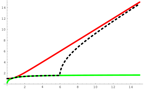
Figure 1: The two approximate solutions of Eq. (4.2) and a rough attempt to join them appropriately. The red curve is obtained in the case $\alpha=0$, the green is for $\beta=0$, so that the red is appropriate when $\delta<<1$ and the green when $\delta>>1$. The black dashed is obtained by using the first solution for $\delta<1$, which happens at the beginning and at the end, and the second in the other case. The discontinuity in the derivative results from the rough procedure. This curve should be compared with the ones of Fig. 2, obtained numerically from the full equation.

Figure 2: Numerical integration of the full Eq. (4.2) when $\alpha=0.1,\beta=1,r_{\rm start}=1$, for various values of $G_{\rm start}$. Units are arbitrary. Comparison with Fig. 1 shows that the qualitative analysis is correct.

- (1) Reuter M 1998 Phys. Rev. D 57 971
- (2) Lauscher O and Reuter M 2005 hep-th/0511260.
- (3) Niedermaier M and Reuter M 2006 Liv. Rev. Rel. 5
- (4) Niedermaier M 2007 Class. Quantum Grav. 24 R171
- (5) Reuter M and Weyer H 2006 Int. J. Mod. Phys. D 15 2011
- (6) Reuter M and Weyer H 2004 Phys. Rev. D 69 104022
- (7) Bonanno A, Esposito G and Rubano C 2004 Class. Quantum Grav. 21 5005
- (8) York J 1972 Phys. Rev. Lett. 28 1082
- (9) Gibbons G W and Hawking S W, Phys. Rev. D 15 2752
- (10) Kuchar K V 1994 Phys. Rev. D 50 3961
- (11) Shapiro I L and Takata A 1995 Phys. Rev. D 52 2162
- (12) Dirac P A M 2001 Lectures on Quantum Mechanics (New York: Dover).
- (13) Faraoni V, Gunzig E and Nardone P 1998 Fund. Cosmic Phys. 20 121 (gr-qc/9811047)
- (14) DeWitt B S 1967 Phys. Rev. 160 1113
- (15) Anderson I M, Fels M E and Torre C G 2000 Commun. Math. Phys. 212 653
- (16) Berger B K, Chitre D M, Moncrief V E and Nutku Y 1972 Phys. Rev. D 5 2467
- (17) Bonanno A and Reuter M 2000 Phys. Rev. D 62 043008
- (18) Giovanelli R, Haynes M P, Herter T, Vogt N P, Wegner G, Salzer J J, Da Costa L N and Freudling W 1997 Astron. J. 113 22
- (19) Clowe D, Bradac M, Gonzalez A H, Markevitch M, Randall S W, Jones C and Zaritsky D “A direct empirical proof of the existence of dark matter” (astro-ph/0608407).