Weakly polydisperse systems: Perturbative phase diagrams that include the critical region

Abstract

The phase behaviour of a weakly polydisperse system, such as a colloid with a small spread of particle sizes, can be related perturbatively to that of its monodisperse counterpart. I show how this approach can be generalized to remain well-behaved near critical points, avoiding the divergences of existing methods and giving access to some of the key qualitative features of polydisperse phase equilibria. The analysis explains also why in purely size-polydisperse systems the critical point is, unusually, located very near the maximum of the cloud and shadow curves.

PACS numbers: 64.10.+h, 68.35.Rh, 82.70.-y, 05.20.-y

Most soft materials are inherently polydisperse: spherical colloids have a spread of diameters, polymers an effectively continuous distribution of chain lengths etc. The effects of polydispersity on equilibrium phase behaviour are both of fundamental interest and of relevance to production, processing and shelf life of foodstuffs, personal hygiene products, paints and coatings etc. Careful sample preparation can reduce polydispersity, to e.g. diameter standard deviations of around 5% for colloids Pusey and van Megen (1986), but not eliminate it. Existing theories that calculate the effects of such weak polydispersity by expanding around the phase equilibria of a monodisperse reference system Evans et al. (1998); Evans (2001) have proved useful, but break down around critical points (CPs) where the relevant prefactors scale with the compressibility. The critical region can be studied alternatively by a Landau expansion Rascón and Cates (2003); while not limited to weak polydispersity, this is impractical for all but the simplest models. Generic tools for predicting polydispersity effects also in the critical region would clearly be useful: as we will see, the qualitatively distinct features of polydisperse phase behaviour manifest themselves most clearly here, and critical parameters can be estimated reliably from simulations Wilding and Sollich (2004); Wilding et al. (2004) and used to constrain theoretical models. My aim here is to supply such a tool, by formulating a perturbative approach that remains applicable in the critical region. The approach allows for the prediction of the full phase behaviour of generic weakly polydisperse materials from that of the monodisperse reference system. As a by-product, the analysis rationalizes previously unexplained peculiarities in the phase behaviour of purely size-polydisperse system. The key idea is that, because a polydisperse system has a critical temperature different from its monodisperse counterpart, one has to allow perturbations not just of the coexisting densities but also of temperature.

Denote the polydisperse attribute, e.g. particle diameter, by $\sigma$, and its average in the parent phase that is allowed to phase separate by $\sigma_{0}$. In terms of the scaled deviations from the parental mean, $\epsilon=(\sigma-\sigma_{0})/\sigma_{0}$, the normalized parent size distribution $p(\epsilon)$ then has zero mean and, by the assumption of weak polydispersity, small variance $w=\int\!d\epsilon\,p(\epsilon)\epsilon^{2}$. We describe a generic phase of the system by its (number) density distribution $\rho(\epsilon)$. Its excess Helmholtz free energy density in units of $k_{\rm B}T$, $\tilde{f}_{\rm poly}$, is a functional of $\rho(\epsilon)$ and an ordinary function of inverse temperature $\beta=1/k_{\rm B}T$. For weak polydispersity this can be expanded up to $\mathcal{O}(\epsilon^{2})$ as Evans et al. (1998); Evans (2001):

$$\tilde{f}_{\rm poly}([\rho(\epsilon)],\beta)=\tilde{f}+A\rho_{1}+B\rho_{2}+C\rho_{1}^{2}$$ (1)

Here the monodisperse reference free energy $\tilde{f}$ is a function of the overall number density $\rho_{0}=\int\!d\epsilon\,\rho(\epsilon)$ and $\beta$, as are the coefficients $A$, $B$, $C$; we abbreviate $\rho\equiv\rho_{0}$ below. The higher-order moment densities are defined as $\rho_{n}=\int\!d\epsilon\,\rho(\epsilon)\epsilon^{n}$ ($n=1,2$). From $\tilde{f}_{\rm poly}$ one finds the excess chemical potentials $\tilde{\mu}(\epsilon)=\delta\tilde{f}_{\rm poly}/\delta\rho(\epsilon)$

$$\tilde{\mu}(\epsilon)=\tilde{f}_{\rho}+A_{\rho}\rho_{1}+B_{\rho}\rho_{2}+C_{\rho}\rho_{1}^{2}+(A+2C\rho_{1})\epsilon+B\epsilon^{2}$$

where subscripts indicate derivatives, i.e. $\tilde{f}_{\rho}\equiv\partial\tilde{f}/\partial\rho$ etc. Equality of the full chemical potentials $\mu(\epsilon)=\ln\rho(\epsilon)+\tilde{\mu}(\epsilon)$ then implies that phases in coexistence have density distributions differing by a factor of the form $\exp(\lambda_{0}+\lambda_{1}\epsilon+\lambda_{2}\epsilon^{2})$, as expected from the moment structure of (1) Sollich and Cates (1998); Sollich et al. (2001). The pressure $\Pi_{\rm poly}=\rho+\int\!d\epsilon\,\rho(\epsilon)\tilde{\mu}(\epsilon)-\tilde{f}_{\rm poly}$ becomes

$$\Pi_{\rm poly}=\Pi+A_{\rho}\rho\rho_{1}+B_{\rho}\rho\rho_{2}+(C_{\rho}\rho+C)\rho_{1}^{2}$$ (2)

with the monodisperse reference pressure $\Pi=\rho+\rho\tilde{f}_{\rho}-\tilde{f}$.

In a polydisperse system the monodisperse binodal splits into cloud and shadow curves Sollich (2002). The former records the density of the majority phase at the onset of coexistence, the latter that of the incipient phase. The cloud phase is then identical to the parent, with a density distribution of the form $\rho\,p(\epsilon)$, while that of the coexisting shadow can be written $\rho\,p(\epsilon)\exp(\lambda_{0}+\lambda_{1}\epsilon+\lambda_{2}\epsilon^{2})$. Equality of pressures and of the $\mathcal{O}(\epsilon^{0})$, $\mathcal{O}(\epsilon^{1})$ and $\mathcal{O}(\epsilon^{2})$ terms in the chemical potentials $\mu(\epsilon)$ gives the conditions

$$\Pi+wB_{\rho}\rho^{2} = \Pi^{\prime}+A_{\rho}^{\prime}\rho^{\prime}\rho_{1}^{\prime}+B_{\rho}^{\prime}\rho^{\prime}\rho_{2}^{\prime}+(C_{\rho}^{\prime}\rho^{\prime}+C^{\prime})\rho_{1}^{\prime}{}^{2}$$

$$\tilde{f}_{\rho}+wB_{\rho}\rho = \tilde{f}_{\rho}^{\prime}+A_{\rho}^{\prime}\rho_{1}^{\prime}+B_{\rho}^{\prime}\rho_{2}^{\prime}+C_{\rho}^{\prime}\rho_{1}^{\prime}{}^{2}+\lambda_{0}$$

$$A = A^{\prime}+2C^{\prime}\rho_{1}^{\prime}+\lambda_{1}$$

$$B = B^{\prime}+\lambda_{2}$$

where unprimed/primed quantities relate to the cloud and shadow phase, respectively, e.g. $\rho^{\prime}$, $\rho_{1}^{\prime}$, $\rho_{2}^{\prime}$ are density moments in the shadow and $A_{\rho}\equiv A_{\rho}(\rho,\beta)$, $A_{\rho}^{\prime}\equiv A_{\rho}(\rho^{\prime},\beta)$; we have used that $\rho_{1}=\rho\langle\epsilon\rangle=0$ and $\rho_{2}=\rho\langle\epsilon^{2}\rangle=w\rho$ in the cloud.

The basis of the perturbation expansion is the monodisperse phase coexistence, with coexisting densities $\rho$, $\rho^{\prime}=\rho\exp(\lambda_{0})$ at temperature $\beta$. One then has $w=\rho_{1}^{\prime}=\rho_{2}^{\prime}=0$ and the Lagrange multipliers become $\lambda_{0}=\tilde{f}_{\rho}-\tilde{f}_{\rho}^{\prime}\equiv\Delta\tilde{f}_{\rho}$, $\lambda_{1}=A-A^{\prime}\equiv\Delta A$, $\lambda_{2}=B-B^{\prime}\equiv\Delta B$. The $\Delta$-notation indicates differences between coexisting monodisperse phases. When the parent is made polydisperse, $\rho$ is perturbed to the cloud point density $\rho_{\rm c}=\rho+\delta\rho_{\rm c}$, and the Lagrange multipliers to $\lambda_{0}=\Delta\tilde{f}_{\rho}+\delta\lambda_{0}$, $\lambda_{1}=\Delta A+\delta\lambda_{1}$, $\lambda_{2}=\Delta B+\delta\lambda_{2}$. Expanding to linear order in all small quantities including $w$, the shadow moments become $\rho_{\rm s}^{\prime}=\rho^{\prime}+\delta\rho_{\rm s}^{\prime}$ with

$$\delta\rho_{\rm s}^{\prime}=\rho^{\prime}\{\delta\rho_{\rm c}/\rho+\delta\lambda_{0}+w[{\textstyle\frac{1}{2}}(\Delta A)^{2}+\Delta B]\}$$ (3)

and $\rho_{1}^{\prime}=w\rho^{\prime}\Delta A$, $\rho_{2}^{\prime}=w\rho^{\prime}$. One now inserts these into the four phase coexistence conditions above and expands, crucially also allowing a temperature shift $\beta\to\beta+\delta\beta$. The fourth conditions only serves to determine $\delta\lambda_{2}$ so can be omitted. The third condition reduces to

$$A_{\rho}\delta\rho_{\rm c}-A_{\rho}^{\prime}\delta\rho_{\rm s}^{\prime}+\Delta A_{\beta}\,\delta\beta=2w\rho^{\prime}C^{\prime}\Delta A+\delta\lambda_{1}$$ (4)

while the first two yield, after eliminating $\delta\lambda_{0}$ in favour of $\delta\rho_{\rm s}^{\prime}$ using (3),

$$\!\!\!\!\!\!\Pi_{\rho}\delta\rho_{\rm c}-\Pi_{\rho}^{\prime}\delta\rho_{\rm s}^{\prime}+\Delta\Pi_{\beta}\,\delta\beta=$$

$$\ \ =w[A_{\rho}^{\prime}\rho^{\prime 2}\Delta A-\Delta(B_{\rho}\rho^{2})]$$

$$\!\!\!\!\!\!(\tilde{f}_{\rho\rho}+1/\rho)\delta\rho_{\rm c}-(\tilde{f}_{\rho\rho}^{\prime}+1/\rho^{\prime})\delta\rho_{\rm s}^{\prime}+\Delta\tilde{f}_{\rho\beta}\,\delta\beta=$$

$$\ \ =w\{A_{\rho}^{\prime}\rho^{\prime}\Delta A-(\Delta A)^{2}/2-\Delta(B_{\rho}\rho)-\Delta B\}$$

The cofficients involving $\tilde{f}$ and $\Pi$ can be written in terms of the full monodisperse free energy density including the ideal part, $f=\rho(-1+\ln\rho)+\tilde{f}$: $\tilde{f}_{\rho\rho}+1/\rho=f_{\rho\rho}$, $\tilde{f}_{\rho\beta}=f_{\rho\beta}$, $\Pi_{\rho}=\rho f_{\rho\rho}$ and $\Pi_{\beta}=\rho f_{\rho\beta}-f_{\beta}$. Taking appropriate linear combinations to eliminate $\delta\rho_{\rm c}$ or $\delta\rho_{\rm s}^{\prime}$ then gives

$$\!\!\!\!\!\!f_{\rho\rho}\delta\rho_{\rm c}+[f_{\rho\beta}-\Delta f_{\beta}/\Delta\rho]\,\delta\beta=$$ (5)

$$\ \ =w\{\rho^{\prime}[{\textstyle\frac{1}{2}}(\Delta A)^{2}+\Delta B]/\Delta\rho-\rho B_{\rho}\}$$

$$\!\!\!\!\!\!f_{\rho\rho}^{\prime}\delta\rho_{\rm s}^{\prime}+[f_{\rho\beta}^{\prime}-\Delta f_{\beta}/\Delta\rho]\,\delta\beta=$$ (6)

$$\ \ =w\{\rho[{\textstyle\frac{1}{2}}(\Delta A)^{2}+\Delta B]/\Delta\rho-\rho^{\prime}B_{\rho}^{\prime}-\rho^{\prime}A_{\rho}^{\prime}\Delta A\}$$

If temperature is held constant ($\delta\beta=0$), one retrieves Evans’ results Evans (2001) for the cloud and shadow density shifts. This approach breaks down at the CP because $1/f_{\rho\rho}$ and $1/f_{\rho\rho}^{\prime}$, which are proportional to the compressibilities in the monodisperse reference phases, diverge.

In the more general setup here we can choose a prescription for $\delta\lambda_{1}=\mathcal{O}(w)$ and deduce the temperature shift $\delta\beta$, which will be of the same order. This freedom does not mean that the perturbation theory is ill-defined. In fact, at a fixed perturbed temperature $\beta_{0}=\beta+\delta\beta$ away from the CP, the results are independent of $\delta\beta$. To see this for e.g. the cloud point density, write (5) as

$$\rho_{\rm c}(\beta_{0})=\rho(\beta)+\rho_{\beta}(\beta)\delta\beta+wR(\beta)$$ (7)

The function $wR(\beta)$ is the r.h.s. of (5) divided by $f_{\rho\rho}$, with the $\beta$-dependence of the monodisperse coexisting densities $\rho$ and $\rho^{\prime}$ inserted. That the prefactor of $\delta\beta$ must equal the derivative $\rho_{\beta}\equiv d\rho/d\beta$ along the monodisperse binodal follows by setting $w=0$, in which case there is no additional polydispersity-induced shift. Now if $\delta\beta=0$ Evans (2001), $\rho_{\rm c}(\beta_{0})=\rho(\beta_{0})+wR(\beta_{0})$. This agrees to $\mathcal{O}(w)$ with (7), for any temperature shift $\delta\beta=\mathcal{O}(w)$, since $\rho(\beta_{0})=\rho(\beta)+\rho_{\beta}(\beta)\delta\beta+\mathcal{O}(w^{2})$; the difference between $R(\beta)$ and $R(\beta_{0})$ likewise only gives $\mathcal{O}(w^{2})$ corrections.

To guide the choice of $\delta\lambda_{1}$ one can use the intuition that in a reliable perturbation theory corresponding monodisperse and polydisperse state points should be mapped to each other. At the CP, where cloud and shadow become identical, also their size distributions do, so we must have $\lambda_{1}=\Delta A+\delta\lambda_{1}=\delta\lambda_{1}=0$. This suggests taking $\delta\lambda_{1}=0$ throughout the phase diagram; to eliminate the function $C$ from (4), however, we choose

$$\delta\lambda_{1}=-2w\rho^{\prime}C^{\prime}\Delta A$$ (8)

which still vanishes at the CP.

Equations (4–6) with the choice (8) constitute our generalized perturbation theory; the set of three linear equations is easily solved for $\delta\rho_{\rm c}$, $\delta\rho_{\rm s}^{\prime}$, $\delta\beta$. I show below that the resulting perturbations do remain finite in the critical region for systems with classical critical behaviour. This encompasses a large variety of models used to describe polydisperse complex fluids, such as van der Waals theory for liquids, free volume theory for colloid-polymer mixtures, the Flory-Huggins and Wertheim’s statistical associating fluid theories for polymers etc (see references in Sollich (2002)). For monodisperse reference systems with non-classical critical behaviour one expects that polydispersity will Fisher-renormalize the critical exponents Kita et al. (1997), multiplying them by $1/(1-\alpha)$. For small $w$ a crossover from the monodisperse to the polydisperse exponents should then occur very close to the CP, and this will not be accounted for by our perturbation theory. Studying this crossover is an interesting issue for future work. Because the specific heat exponent $\alpha\approx 0.11$ is small in $d=3$, however, the quantitative effects of Fisher renormalization may well be small enough for the perturbative approach to remain an accurate approximation.

To obtain an explicit expression for the CP shift due to polydispersity, we start by assuming a smooth (Landau-like) expansion of $f$ near criticality. The coexisting densities then go as $\rho-\rho^{*}=-(\rho^{\prime}-\rho^{*})=[2(\beta-\beta^{*})/b]^{1/2}$ to leading order, with $b$ some constant; asterisks denote quantities at the CP. Defining $r=[2(\beta-\beta^{*})/b]^{1/2}$, we can then write $\rho-\rho^{*}=r+ar^{2}$, $\rho^{\prime}-\rho^{*}=-r+ar^{2}$, $\beta=\beta^{*}+\frac{1}{2}br^{2}$ to $\mathcal{O}(r^{2})$. The coefficient $b$ is given by $b=-f^{*}_{\rho\rho\rho\rho}/(3f^{*}_{\rho\rho\beta})$; $a$ will cancel to the order we require. To expand our equations for small $r$ write (4), together with (5,6) divided by $\Delta\rho$, in matrix form $\bm{M}\bm{\delta}=w\bm{v}$. Here $\bm{\delta}^{\text{T}}=(\delta\rho_{\rm c},\delta\rho_{\rm s}^{\prime},\delta\beta)$ and $\bm{v}$ gathers the appropriate right-hand sides. Substituting the above expansions for $\rho$, $\rho^{\prime}$, $\beta$ and using $f^{*}_{\rho\rho}=f^{*}_{\rho\rho\rho}=0$ at the CP then yields $\bm{M}=\bm{M}^{*}+\bm{M}^{*}_{r}r+\ldots$, $\bm{v}=\bm{v}^{*}+\bm{v}^{*}_{r}r+\ldots$ with

$$\bm{M}^{*}=\left(\begin{array}[]{rrr}A^{*}_{\rho}&-A^{*}_{\rho}&0\\ 0&0&\frac{1}{2}f^{*}_{\rho\rho\beta}\\ 0&0&-\frac{1}{2}f^{*}_{\rho\rho\beta}\end{array}\right),\quad\bm{v}^{*}=\left(\begin{array}[]{r}0\\ V\\ -V\end{array}\right)$$ (15)

where $V=\frac{1}{2}\rho^{*}(A_{\rho}^{*}{}^{2}-B_{\rho\rho}^{*})-B^{*}_{\rho}$. We want to deduce from this the expansion of the solution vector, $\bm{\delta}=\bm{\delta}^{*}+r\bm{\delta}^{*}_{r}+\ldots$ Because $\bm{M}^{*}$ is degenerate, the zeroth order $\bm{M}^{*}\bm{\delta}^{*}=w\bm{v}^{*}$ fixes the $\delta\beta$-component of $\bm{\delta}^{*}$ as

$$\delta\beta^{*}=w[\rho^{*}(A_{\rho}^{*}{}^{2}-B_{\rho\rho}^{*})-2B^{*}_{\rho}]/f^{*}_{\rho\rho\beta}$$ (16)

and otherwise (only) tells us that the other components must be equal, $\delta\rho_{\rm c}=\delta\rho_{\rm s}^{\prime}\equiv\delta\rho^{*}$. This is as it should be: we built the perturbation theory to map the monodisperse CP to the polydisperse CP, where $\rho_{\rm c}=\rho_{\rm s}^{\prime}$. Mathematically it follows from the vanishing of the first component of $\bm{v}^{*}$, confirming the intuition that $\delta\lambda_{1}$ needs to be chosen to make the r.h.s. of (4) zero at the CP.

To determine $\delta\rho^{*}$, we use the $\mathcal{O}(r)$ condition $\bm{M}^{*}\bm{\delta}^{*}_{r}+\bm{M}^{*}_{r}\bm{\delta}^{*}=w\bm{v}_{r}^{*}$. Multiplying from the left by $\bm{e}^{\text{T}}=(0,1,1)$ eliminates the first term and gives $\bm{e}^{\text{T}}\bm{M}^{*}_{r}\bm{\delta}^{*}=w\bm{e}^{\text{T}}\bm{v}^{*}_{r}$. By inserting the explicit expressions for $\bm{M}^{*}_{r}$ and $\bm{v}^{*}_{r}$ from the small-$r$ expansion and the form $\bm{\delta}^{*}=(\delta\rho^{*},\delta\rho^{*},\delta\beta^{*})^{\text{T}}$ one then finds

$$f^{*}_{\rho\rho\rho\rho}\delta\rho^{*}+f^{*}_{\rho\rho\rho\beta}\delta\beta^{*}=w[3A^{*}_{\rho}{}^{2}-3B^{*}_{\rho\rho}+\rho^{*}(3A^{*}_{\rho}A^{*}_{\rho\rho}-B^{*}_{\rho\rho\rho})]$$

Together with (16) this gives the desired shifts of the critical density, $\delta\rho^{*}$, and critical temperature, $\delta\beta^{*}$; these results can be checked to agree with the general polydisperse CP criterion Sollich (2002), expanded directly for small $w$. Both shifts $\delta\rho^{*}$ and $\delta\beta^{*}$ are $\mathcal{O}(w)$, so that the loci of the CPs for increasing $w$ depart from the monodisperse CP along a line of nontrivial slope in the $(\rho,\beta)$ plane.

Taking the expansion further, we can obtain the slope of the cloud and shadow curves at the CP, and the location of their maxima. Both are related to $\delta\beta^{*}_{r}=d(\delta\beta)/dr|_{r=0}$, the $\delta\beta$-component of $\bm{\delta}^{*}_{r}$. This follows after some algebra from the first order equation $\bm{M}^{*}\bm{\delta}^{*}_{r}+\bm{M}^{*}_{r}\bm{\delta}^{*}=w\bm{v}_{r}^{*}$ together with the known $\bm{\delta}^{*}$ as

$$\delta\beta^{*}_{r}=-w\,A^{*}_{\rho}(2A^{*}_{\rho}+\rho^{*}A^{*}_{\rho\rho})/f^{*}_{\rho\rho\beta}$$ (17)

The slope of the cloud curve, plotted as $\beta$ vs $\rho_{\rm c}$, is $d(\beta+\delta\beta)/d(\rho+\delta\rho_{\rm c})=[d(\beta+\delta\beta)/dr][d(\rho+\delta\rho_{\rm c})/dr]^{-1}$. At the critical point, the first factor equals $\delta\beta_{r}^{*}$. This is $\mathcal{O}(w)$, so we only need the $\mathcal{O}(w^{0})$ contribution, $d\rho/dr=1$, of the second factor to find the cloud slope at the CP as $\delta\beta_{r}^{*}$. The shadow slope has the same modulus but opposite sign since $d\rho^{\prime}/dr=-1$. For the cloud and shadow maxima we want to find $r$ such that $d(\beta+\delta\beta)/dr=0$, giving $br+\delta\beta_{r}^{*}=0$ or $r=-\delta\beta^{*}_{r}/b$. Because this is $\mathcal{O}(w)$, it is correct to replace $\delta\beta_{r}$ by $\delta\beta_{r}^{*}$ as we have done. It follows that the cloud and shadow maxima are to $\mathcal{O}(w)$ located at $\rho_{{\rm c},{\rm s}}=\rho^{*}+\delta\rho^{*}\mp\delta\beta^{*}_{r}/b$, i.e. equidistant either side of the polydisperse CP.

Finally we turn to purely size-polydisperse (“scalable” Evans (2001)) systems, in which the interaction potential remains unchanged when the diameters $\sigma_{i}$ and position vectors of all particles are scaled by a common factor. For pair interactions, this holds if the dependence on distance $r_{ij}$ of the potential between two particles $i$ and $j$ can be written as $v_{ij}(r_{ij})=\Phi(r_{ij}/\ell(\sigma_{i},\sigma_{j}))$ with the interaction distance $\ell$ a homogeneous function of first degree like $\ell=(\sigma_{i}+\sigma_{j})/2$ or $\ell=(\sigma_{i}\sigma_{j})^{1/2}$. This includes e.g. polydisperse (additive) hard spheres, or size-polydisperse Lennard-Jones mixtures. Simulations and theoretical calculations Bellier-Castella et al. (2000); Wilding and Sollich (2004); Wilding et al. (2004); Fantoni et al. (2006) show that for such systems, unusually in the presence of polydispersity, the critical point is located very near the maximum of the cloud and shadow curves (and thus also close to the maximum of a plot of pressure versus temperature at the onset of phase coexistence Bellier-Castella et al. (2000); Rascón and Cates (2003)). Moreover, plotted in terms of volume fraction instead of density, cloud and shadow curves almost coincide Bellier-Castella et al. (2000); Wilding and Sollich (2004); Wilding et al. (2004); Fantoni et al. (2006).

This behaviour is fully predicted by our $\mathcal{O}(w)$ perturbation theory. As regards the location of the CP, we need only use that in size-polydisperse systems Evans (2001)

$$A=3(\Pi/\rho-1)=3(f_{\rho}-f/\rho-1)$$ (18)

Working out $A_{\rho}$ and $A_{\rho\rho}$, substituting into (17) and using $f^{*}_{\rho\rho}=f^{*}_{\rho\rho\rho}=0$ then gives $\delta\beta^{*}_{r}=0$. The cloud and shadow slopes at the CP, $\pm\delta\beta^{*}_{r}$, thus vanish to $\mathcal{O}(w)$, so that the CP must be at their maximum as claimed.

To see the coincidence of the volume fraction representations of cloud and shadow, we measure densities in units of $(\pi\sigma_{0}^{3}/6)^{-1}$ so that the volume fraction can be written $\phi=\int\!d\epsilon\,\rho(\epsilon)(1+\epsilon)^{3}$. Expanding to $\mathcal{O}(w)$ gives for the cloud volume fraction $\phi_{\rm c}=\rho(1+3w)+\delta\rho_{\rm c}$, while for the shadow $\phi_{\rm s}=\rho^{\prime}(1+3w\Delta A+3w)+\delta\rho_{\rm s}^{\prime}$. One can now write equations (4–6) in terms of the volume fraction shifts $\delta\phi_{\rm c}=\phi_{\rm c}-\rho$ and $\delta\phi_{\rm s}^{\prime}=\phi_{\rm s}^{\prime}-\rho^{\prime}$. Swapping $\rho$ and $\rho^{\prime}$ gives equations for $\delta\phi_{\rm c}^{\prime}$ and $\delta\phi_{\rm s}$; coincidence requires that $\delta\phi_{\rm c}=\delta\phi_{\rm s}$ and $\delta\phi_{\rm c}^{\prime}=\delta\phi_{\rm s}^{\prime}$, i.e. any point on the monodisperse binodal is perturbed into cloud and shadow points with identical volume fractions. The original and swapped equations turn out to differ by a term proportional to $\rho\Delta A/\Delta\rho+3\rho^{\prime}f_{\rho\rho}^{\prime}-\rho^{\prime}A_{\rho}^{\prime}$ on the r.h.s.; from (18) this indeed vanishes for size-polydisperse systems. To ensure that also the temperature shift $\delta\beta$ is the same, one needs to modify slightly the choice (8) of $\delta\lambda_{1}$, taking e.g.

$$\delta\lambda_{1}=w\rho^{\prime}\Delta A(-2C^{\prime}+3A_{\rho}^{\prime})$$ (19)

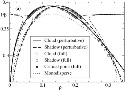
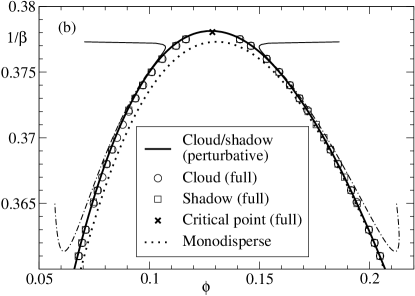
Figure 1: (a) Cloud and shadow curves for a model of a Lennard-Jones mixture with polydispersity in both particle diameters and interaction strengths. Symbols: full non-perturbative solution. Thick lines: perturbation theory with choice (19); using (8) only gives noticeable differences for the high-density part of the shadow curve (dash-dotted line). Thin lines: constant-$\beta$ approach of Evans (2001). Dotted line: monodisperse binodal. (b) Similar plot for a purely size-polydisperse mixture, in the volume fraction representation. Dash-dotted line: unregularized perturbation theory.

To illustrate the theory we show in Fig. 1(a) the predictions for a Lennard-Jones mixture with polydispersity in both particle diameters and interaction strengths, modelled with a moment excess free energy Sollich and Cates (1998); Sollich et al. (2001) as in Wilding et al. (2005, 2006), for a uniform (“top hat”) size distribution $p(\epsilon)$ of width $w^{1/2}=0.07$. The generalized perturbation theory produces cloud and shadow curves with smoothly connecting sub- and super-critical branches, avoiding the divergences near the monodisperse CP of the constant-$\beta$ approach Evans (2001). Comparing with the symbols, our perturbation theory is quantitatively closer to the full solution of the polydisperse phase equilibrium conditions also elsewhere, in particular for the high-density branch of the shadow curve. The overall level of agreement is quite remarkable given that the shifts from the monodisperse reference system (dotted line) are substantial.

Fig. 1(b) shows similar results for a mixture with pure size polydispersity Wilding and Sollich (2004); Wilding et al. (2004). In the volume fraction representation cloud and shadow curves coincide as predicted, and the CP is very near their maximum. Again, our approach avoids divergences in this region and is quantitatively accurate even for the substantial degree of polydispersity $w^{1/2}=0.2$ considered here, i.e. a size standard that is $20\%$ of the mean. The dash-dotted line gives the raw results of the perturbation theory; the unphysical upward curvature comes from an increase in the temperature shifts $|\delta\beta|$. This illustrates that, away from the CP where we should have $\delta\lambda_{1}=0$, it is not obvious how to choose $\delta\lambda_{1}$ to extract the most reliable predictions for finite $w$. Intuitively, one expects temperature shifts to be needed primarily in the critical region and to become smaller elsewhere. This can be enforced by e.g. taking the raw $\delta\beta$ and using a soft thresholding function so that values with $|\delta\beta|>|\delta\beta^{*}|$ are reassigned to be no larger than $2|\delta\beta^{*}|$; $\delta\rho_{\rm c}$ and $\delta\rho_{\rm s}^{\prime}$ are then recalculated from (5,6). The thick line in Fig. 1 shows that this gives accurate and physically sensible results.

The approach presented here allows the calculation of full phase diagrams for generic weakly polydisperse systems, giving access to key features such as the separation of the maxima of cloud and shadow from the CP, the differing cloud and shadow slopes at the CP, and the polydispersity-induced shifts of the critical parameters. Even for excess free energies with moment structure it can be helpful in avoiding the computational complexities of a full phase equilibrium calculation Sollich (2002), while remaining quantitatively accurate in a substantial range of polydispersities (up to $20\%$ in Fig. 1) that includes typical experimental values Pusey and van Megen (1986). The theory also generalizes easily to phase equilibria inside the coexistence region, as well as systems with several polydisperse attributes.

References

Pusey and van Megen (1986)
P. N. Pusey and
W. van Megen,
Nature 320,
340 (1986).
Evans et al. (1998)
R. M. L. Evans,
D. J. Fairhurst,
and W. C. K.
Poon, Phys. Rev. Lett.
81, 1326 (1998).
Evans (2001)
R. M. L. Evans,
J. Chem. Phys. 114,
1915 (2001).
Rascón and Cates (2003)
C. Rascón
and M. E. Cates,
J. Chem. Phys. 118,
4312 (2003).
Wilding and Sollich (2004)
N. B. Wilding and
P. Sollich,
Europhys. Lett. 67,
219 (2004).
Wilding et al. (2004)
N. B. Wilding,
M. Fasolo, and
P. Sollich,
J. Chem. Phys. 121,
6887 (2004).
Sollich and Cates (1998)
P. Sollich and
M. E. Cates,
Phys. Rev. Lett. 80,
1365 (1998).
Sollich et al. (2001)
P. Sollich,
P. B. Warren,
and M. E. Cates,
Adv. Chem. Phys. 116,
265 (2001).
Sollich (2002)
P. Sollich,
J. Phys. Cond. Matt. 14,
R79 (2002).
Kita et al. (1997)
R. Kita,
T. Dobashi,
T. Yamamoto,
M. Nakata, and
K. Kamide,
Phys. Rev. E 55,
3159 (1997).
Bellier-Castella
et al. (2000)
L. Bellier-Castella,
H. Xu, and
M. Baus, J. Chem. Phys. 113, 8337
(2000).
Fantoni et al. (2006)
R. Fantoni,
D. Gazzillo,
A. Giacometti,
and P. Sollich,
J. Chem. Phys. 125,
164504 (2006).
Wilding et al. (2005)
N. B. Wilding,
P. Sollich, and
M. Fasolo,
Phys. Rev. Lett. 95,
155701 (2005).
Wilding et al. (2006)
N. B. Wilding,
P. Sollich,
M. Fasolo, and
M. Buzzacchi,
J. Chem. Phys. 125,
014908 (2006).